Research on Energy Futures Hedging Strategies for Electricity Retailers’ Risk Based on Monthly Electricity Price Forecasting

Abstract

The widespread adoption of electricity market trading platforms has enhanced the standardization and transparency of trading processes. As markets become more liberalized, regulatory policies are phasing out protective electricity pricing mechanisms, leaving retailers exposed to price volatility risks. In response, demand for risk management tools has grown significantly. Futures contracts serve as a core instrument for managing risks in the energy sector. This paper proposes a futures-based risk hedging model grounded in electricity price forecasting. A price prediction model is constructed using historical data from electricity markets and energy futures, with SHAP values used to analyze the transmission effects of energy futures prices on monthly electricity trading prices. The Monte Carlo simulation method, combined with a t-GARCH model, is applied to calculate CVaR and determine optimal portfolio weights for futures products. This approach captures the volatility clustering and fat-tailed characteristics typical of energy futures returns. To validate the model’s effectiveness, an empirical analysis is conducted using actual market data. By forecasting electricity price trends and formulating futures strategies, the study evaluates the hedging and profitability performance of futures trading under different market conditions. Results show that the proposed model effectively mitigates risks in volatile market environments.

1. Introduction

As the electricity market gradually opens up, the increasingly complex environment has heightened market uncertainty, making electricity prices more susceptible to changes in supply and demand and other external factors. In countries that have already introduced electricity futures trading, electricity retailers can use electricity futures to hedge against risks arising from electricity price fluctuations, based on the characteristics of electricity pricing [1]. However, in many countries, electricity futures have not yet been launched, and spot electricity markets are not fully developed. As a result, alternative methods for risk hedging must be considered. In this context, fossil fuel futures, which are closely linked to electricity prices, are considered potential tools for risk management.

Contemporary research has progressively addressed the critical challenge of risk mitigation in deregulated electricity markets. As demonstrated in [2], the dual uncertainties in price and trading volume pose substantial threats to corporate financial stability, with conventional hedging instruments like electricity futures proving inadequate due to market illiquidity. This investigation pioneers an innovative risk management framework through the synergistic combination of energy derivatives and weather derivatives. Complementary analysis in [3] employs variance minimization criteria to assess weekly versus monthly hedging efficacy, revealing electricity futures’ underperformance relative to other energy commodities.

Multidimensional investigations have elucidated the intricate price transmission mechanisms between energy commodities and electricity markets. Regarding fossil fuel impacts, empirical evidence from the Guangdong regional market [4] establishes significant positive correlation between monthly electricity and coal prices. The VAR-MGARCH analysis in [5] systematically decouples these dynamic interactions: coal prices exert immediate short-term effects while natural gas predominantly influences price volatility, contrasting with crude oil’s statistically insignificant role. Time-frequency decomposition in [6] further identifies delayed responses in electricity market volatility to fossil fuel market fluctuations, distinguishing renewable-driven spot price dynamics from futures market behavior shaped by natural gas pricing.

Advanced methodologies have enhanced understanding of interconnected energy market risks. Through wavelet coherence analysis, [7] quantifies event-driven spillover effects across temporal scales. A breakthrough in [8] applies dynamic factor modeling to disentangle the co-volatility structure among electricity, fossil fuel, and carbon markets. Critical pathway analysis in [9] maps risk transmission channels, confirming electricity market-mediated impacts of fossil fuels on carbon markets, thereby informing carbon risk mitigation strategies. The natural gas-electricity nexus study [10] reveals futures market leadership effects, substantiating cross-commodity hedging viability through Granger causality analysis.

Cutting-edge forecasting methodologies increasingly integrate cross-domain insights. The hybrid model in [11] synergizes Fourier decomposition with multi-energy price drivers, while comparative analysis in [12] validates accuracy improvements through fossil-renewable energy indicator fusion. References [13,14] both adopt a hybrid framework that integrates signal decomposition with predictive modeling. Reference [15] (SSA-LSTM) demonstrates a streamlined and efficient structure, effectively balancing high predictive accuracy with manageable model complexity. In contrast, [16] (VMD-PSO-LSTM-RF) employs a more sophisticated architecture designed for peak accuracy, utilizing adaptive decomposition, seasonal hyperparameter optimization, and ensemble forecasting to capture the intricate, multi-scale fluctuations in short-term load data within electricity markets. Reference [17] (ARIMA & CNN-Bi-LSTM) follows a distinct comparative validation approach. It provides a robust and practical empirical assessment of traditional versus deep learning models for mid-term electricity consumption forecasting, prioritizing the verification of a feasible methodological framework over the pursuit of ultimate predictive precision. Explainable AI applications in [18,19,20] employ SHAP value analysis to decode complex relationships, including lagged feature impacts, renewable penetration effects on price distributions, and anomaly driving factors. This interpretability framework extends to grid congestion analysis in [21], successfully identifying critical nodal influences and causal pathways. Previous studies have noted the limitations of SHAP-based interpretation in time-series models with multiple lagged variables. Ref. [22] shows that due to the strong correlations among lagged features, SHAP values primarily capture the model’s predictive dependence on historical information rather than the independent effects of individual lags, and therefore should be interpreted with caution under multicollinearity.

Despite these advancements, several critical research gaps remain unaddressed, which this paper aims to fill:

(1)

Lack of Integrated Forecasting-Hedging Frameworks: Existing studies often treat price forecasting and hedging strategy design as separate tasks. There is a need for a cohesive model that directly uses a high-accuracy price forecast to inform and trigger specific, actionable hedging decisions in related energy futures markets.

(2)

Insufficient Exploration of Lagged Price Transmission for Hedging: While the literature acknowledges lead-lag relationships between energy markets [6,10], few studies have quantitatively and systematically mapped these lag cycles with the explicit goal of identifying optimal futures entry points for electricity retailers. The understanding of how the transmission time varies between different fossil fuel futures is limited.

(3)

Absence of Practical, Risk-Adjusted Portfolio Allocation for Electricity Retailers: Previous research on hedging often focuses on minimizing variance or calculating CVaR under standard distributional assumptions. There is a gap in providing electricity retailers with a practical portfolio weight allocation that explicitly balances risk and return, accounting for the heavy-tailed characteristics of energy futures returns, and is validated with real market trading data.

In response to these gaps, this article proposes an integrated futures risk hedging model based on monthly electricity price forecasting. The main contributions are as follows:

(1)

An Integrated Forecasting-Hedging Framework: By developing a hybrid SSA-LSTM model that incorporates energy futures prices, this study not only improves monthly electricity price forecast accuracy but also directly uses the forecasted trend to generate clear signals for futures market operations, creating a closed-loop from prediction to strategy execution.

(2)

Quantification of Lagged Transmission for Strategy Timing: Using SHAP interpretable machine learning on a constructed lag model, this research explicitly uncovers the distinct lag cycles in the price signal transmission from JM (coking coal) and LPG futures to monthly electricity prices. This analysis directly informs the precise timing (specific trading days) for initiating futures positions, a critical component often overlooked in prior work.

(3)

A Practical Risk-Optimized Portfolio Allocation Model: We establish a quantitative risk model using Monte Carlo simulation to calculate CVaR under a t-GARCH assumption, which better captures the fat-tailed nature of energy returns. This model provides electricity retailers with a specific, optimal allocation weight between futures that balances risk control and return stability, moving beyond theoretical hedging to offer actionable decision support.

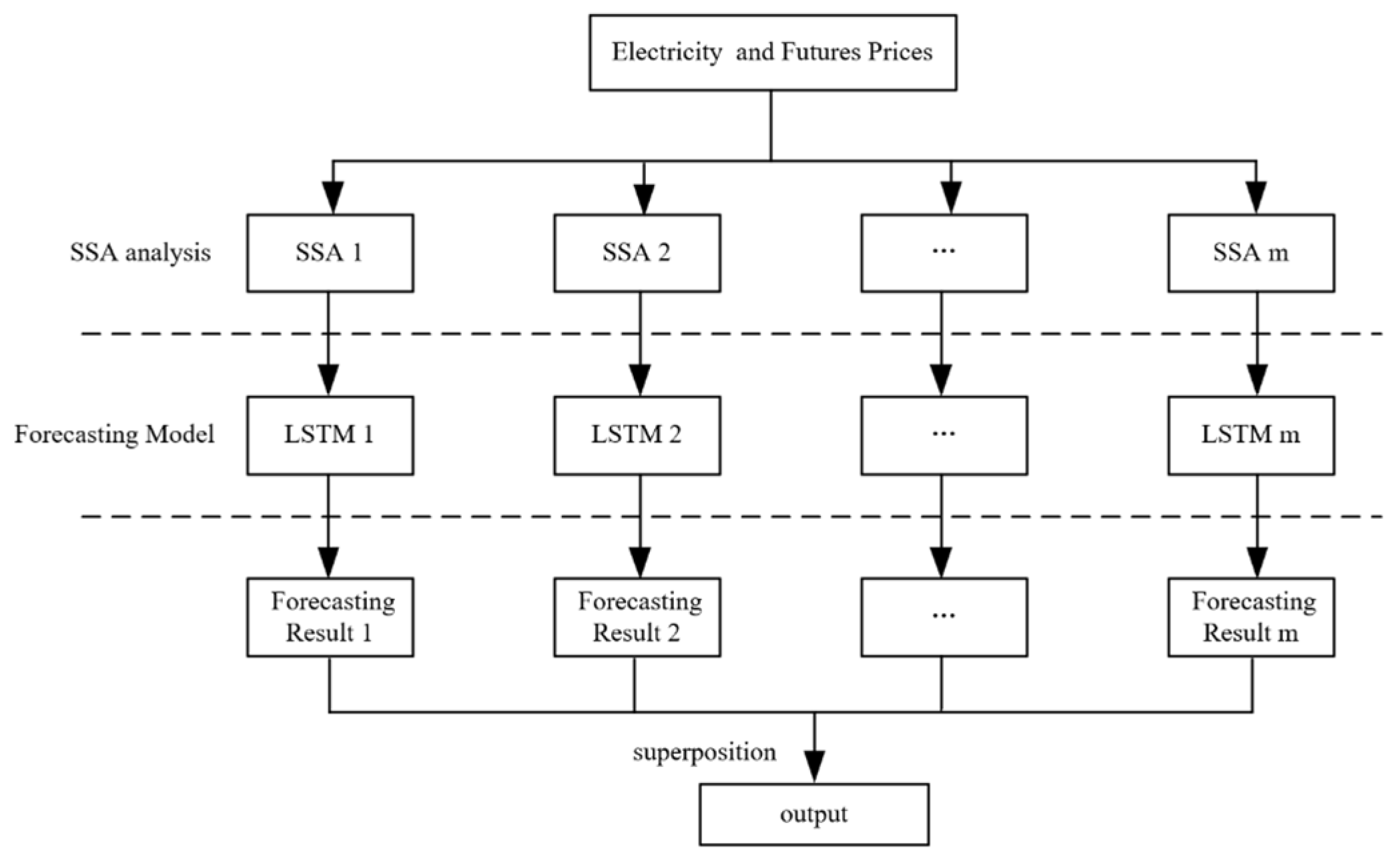
In summary, the integrated risk management framework developed in this study follows a clear logical chain: First, the SSA-LSTM model generates high-precision monthly electricity price forecast paths, which provide the core input and directional guidance for subsequent risk analysis. Next, SHAP interpretability analysis is used to delve into the drivers of price fluctuations, explicitly identifying the intensity and direction of the influence of JM and LPG futures on electricity prices at specific lag periods. This directly determines which futures contracts should be selected for hedging and the optimal entry timing. Finally, based on the forecasted electricity price scenarios and the selected futures contracts, a t-GARCH-based Monte Carlo simulation is employed to calculate the portfolio CVaR, thereby quantifying the results of the first two steps into specific, understandable risk exposure numbers and optimal asset allocation weights for electricity retailers. These three components connect sequentially, collectively forming a complete decision-support system that moves from forecasting and explanation to risk quantification.

The rest of this article is structured as follows: Section 2 develops the monthly electricity price forecasting model using the SSA-LSTM approach. Section 3 analyzes the lagged impact of energy futures on electricity prices using the SHAP model to determine optimal entry timing. Section 4 determines the optimal futures allocation weights by computing the portfolio CVaR through the Monte Carlo method. In Section 5, real market data is used to validate the effectiveness of the proposed method, followed by an in-depth discussion. Section 6 concludes this article. The overall research framework is illustrated in Figure 1.

2. Monthly Electricity Trading Price Forecasting Based on SSA-LSTM

2.1. Monthly Centralized Electricity Prices

Currently, a wide variety of electricity trading products is available. Different trading types have been introduced to meet demand across various time scales, including, annual, quarterly, monthly, weekly, daily, and real-time electricity transactions. These trading products show significant differences in price levels and volatility [23]. Therefore, when designing a futures trading strategy, it is essential first to identify the specific electricity price benchmark corresponding to the selected futures product.

The electricity market is predominantly characterized by medium- and long-term trading, which accounts for over 90% of market-based electricity volume. Among these, monthly centralized trading, which serves as the concluding stage of the medium- and long-term market and is closely linked to dispatch operations, better reflects the overall price trends and supply-demand dynamics of the electricity market. The trading process is as follows: market participants first submit their declared electricity volumes and prices to the trading institution; the institution then organizes buyers’ prices in descending order and sellers’ prices in ascending order to create supply and demand curves. Finally, based on a volume–price matching mechanism, electricity is allocated in the order of the largest price differentials until the price difference reaches zero, at which point matching concludes.

As a unique commodity, electricity prices are highly sensitive to supply and demand conditions. Since coal, oil, and gas remain the dominant fuels for power generation, electricity prices are closely tied to fuel prices. Futures indices, which serve as key market indicators, effectively capture economic conditions and electricity demand levels.

2.2. Multidimensional Long Short-Term Memory Networks

2.2.1. Data Processing and Construction

The quality of the sample data directly affects the accuracy of forecasting results, and more accurate predictions can provide better guidance for futures trading strategies. Therefore, precise feature selection from the raw data is particularly important. After determining the feature variables, data normalization is required to eliminate the impact of differing scales on the forecasting performance and to accelerate the model’s processing speed and training time.

The sample dataset used in this study is from publicly disclosed market data and real futures data obtained from the Wind database. The time range is from 2018 to 2024, with the corresponding monthly centralized electricity trading prices shown in Figure 2. This study employs the Pearson correlation coefficient method to analyze the relationships between variables and monthly centralized electricity prices to select appropriate input features. The calculation results are presented in

Table 1. Correlation Coefficients.

Feature Parameter	Correlation
Annual Bilateral Negotiated Electricity Price	0.6777
Monthly Centralized Bidding Electricity Volume	−0.3174
Generation-side Market Concentration Index	−0.3418
Demand-side Market Concentration Index	−0.1276
Thermal Coal Monthly Average Price	0.6405
JM Futures Monthly Average Price	0.4065
LPG Futures Monthly Average Price	0.6753

.

As shown in Table 1, monthly centralized electricity trading prices exhibit strong correlations with the annual bilateral negotiated electricity price, the thermal coal index, the JM futures index, and the LPG futures index. Accordingly, these variables are selected as input features for the forecasting model in this study.

2.2.2. SSA-LSTM Model

Compared with traditional univariate forecasting models, the LSTM model captures temporal patterns in data more effectively. As illustrated in Figure 3, the network structure consists of a forget gate, an input gate, an output gate, and a cell state. The input gate controls how much the incoming data influences the cell state, the forget gate determines which information is discarded from the cell, and the output gate decides which information is output at the current time step. Their corresponding mathematical expressions are as follows:

$$f_t=\sigma (W_{\mathrm{f}}\cdot [h_{t-1},x_t]+b_{\mathrm{f}})$$

(1)

In Equation (1), $\sigma$ is the sigmoid activation function; $W_{\mathrm{f}}$ is the forget gate weight matrix; is the previous hidden state; $x_t$ is the current input; $b_{\mathrm{f}}$ is the forget gate bias.

$$i_t=\sigma (W_{\mathrm{i}}\cdot [h_{t-1},x_t]+b_{\mathrm{i}})$$

(2)

$${\tilde{C}}_t=\tanh \left(W_{\mathfrak{c}}\cdot [h_{t-1},x_t]+b_{\mathfrak{c}}\right)$$

(3)

In Equations (2) and (3), $i_t$ is the input gate; $W_{\mathrm{i}}$ and $b_{\mathrm{i}}$ are the weight matrix and bias of the input gate, respectively; ${\tilde{C}}_t$ is the candidate cell state; $W_{\mathfrak{c}}$, $b_{\mathfrak{c}}$ are the weight and bias for the tanh transformation.

$$C_t=f_t\cdot C_{t-1}+i_t\cdot {\tilde{C}}_t$$

(4)

In Equation (4), $C_t$ is the updated cell state, and $C_{t-1}$ is the previous cell state.

$$O_t=\sigma \left(W_0\cdot [h_{t-1},x_t]+b_0\right)$$

(5)

$$h_t=O_t\cdot \tanh C_t$$

(6)

In Equations (5) and (6), $O_t$, $W_0$, $b_0$ denote the output gate, its weight matrix, and bias, respectively. $h_t$ is the current hidden state.

As the core components, the network layers can capture the temporal trends in electricity prices and the sequential dependencies between input features. The fully connected layers are better suited for processing high-dimensional time series data, while the dropout layers are employed to prevent overfitting effectively.

Singular Spectrum Analysis (SSA) is a semi-parametric time series decomposition method that enables the precise extraction of complex cyclical components through its adaptive filtering characteristics.

As illustrated in Figure 4, the implementation process involves three key steps: performing SSA decomposition, independently forecasting each decomposed component, and aggregating the forecasts of all components.

The SSA process consists of four main steps:

(1)

Trajectory Matrix Construction (Embedding)

Given the original time series $Y_N$ = $(y_1,y_2,\cdots \cdots ,y_N)$, a trajectory matrix is constructed by setting an embedding dimension L:

$$G=\left[\begin{array}{cccc}{y}_1& y_2& \dots & y_K\\ y_2& y_3& \dots & y_{K+1}\\ ⋮& ⋮& \ddots & ⋮\\ y_L& y_{L+1}& \dots & y_N\end{array}\right]$$

(7)

This step captures the dynamic features of the time series by constructing a high-dimensional phase space.

(2)

Singular Value Decomposition (SVD)

The trajectory matrix G is decomposed using SVD:

$$G=\sum _{i=1}^e{S}_i=\sum _{i=1}^e\sqrt{{\lambda }_i}{U}_i{V}_i^T$$

(8)

where ${\lambda }_i$ are the eigenvalues of the covariance matrix, and the eigenvalues of $G^{T}G$, with $U_i$ and $V_i$ being the left and right singular vectors of matrix G.

(3)

Subgroup Reconstruction

The initial equal-sized matrices $S_i$ are grouped according to their eigenenergy, forming different trend components:

$$G_{I_k}={\displaystyle \sum _{i\in I_k}{S}_i}$$

(9)

(4)

Anti-diagonal Averaging

The anti-diagonal averaging is performed on the reconstructed time series via inverse embedding, and its formula is:

$$g_k=\left\{\begin{array}{c}{\displaystyle \frac{1}{k}}{\displaystyle \sum _{q=1}^{k+1}}{z}_{q,k-q+1}^{\ast },1\le k\le L^{\ast }\\ {\displaystyle \frac{1}{L^{*}}}{\displaystyle \sum _{p=1}^{L^{\ast }}}{z}_{q,k-q+1}^{\ast },L^{\ast }<k\le K^{\ast }\\ {\displaystyle \frac{1}{N-k+1}}{\displaystyle \sum _{p=k-K^{\ast }+1}^{N-K^{\ast }+1}}{z}_{q,k-q+1}^{\ast },K^{\ast }<k\le N\end{array}\right.$$

(10)

To ensure the robustness and interpretability of the results, sensitivity analysis is required to evaluate how the decomposition outcomes respond to changes in window length and the number of components. The sensitivity analysis is shown in Figure 5.

Based on the results of the SSA-LSTM model parameter sensitivity analysis, it can be observed that the window length has a decisive impact on model performance. As the window length increases, the MSE of the model shows a consistently significant decline, decreasing from a maximum of 0.7382 to a minimum of 0.2232. This indicates that a longer window can more effectively capture the trend and periodic components of the time series. In contrast, increasing the number of components leads to a rise in MSE, suggesting that the first few components extracted by SSA already contain most of the useful information.

According to the sensitivity analysis results, appropriately increasing the window length can improve the resolution of the decomposition, enabling the model to more effectively extract the trend and periodic characteristics of the time series. However, an excessively large window size may lead to overfitting, significantly increase computational complexity, and introduce noise components. Considering both model performance and computational efficiency, this study sets the window length to half of the total time series length, ensuring that the trajectory matrix remains approximately symmetric in dimension. This configuration preserves the overall dynamic characteristics of the series while maintaining numerical stability in matrix operations.

By further analyzing the variance contribution of the first eight SSA components, as shown in Figure 6 (SSA decomposition) and Figure 7 (variance contribution), it can be observed that the variance contribution rate of SSA1 reaches 73.55%, indicating that it provides the most significant explanation of the variance in the original time series. The contribution of SSA2 drops sharply to 4.01%, while those of SSA3 to SSA8 are all below 1% and tend to stabilize. The cumulative variance contribution of SSA1 and SSA2 approaches 80%, suggesting that these two components capture the main trend of the series. Although the individual contributions of SSA3–SSA8 are relatively small, they still contain local details and structural information associated with short- and medium-term fluctuations, which should not be neglected. This observation aligns with findings in related SSA-based forecasting studies, where the first few components typically capture the dominant trend and periodic structures, while later components represent noise or minor fluctuations that can be reasonably aggregated or discarded without significant loss of predictive information [20].

Based on the above variance analysis, this study reconstructs SSA1 and SSA2 into a combined low-frequency trend component. This design is theoretically and practically justified for the following reasons: From an information theory perspective, the first two components already account for nearly 80% of the variance in the original series, indicating that they contain most of the systematic information and deterministic trends. Merging them as the core driving component for the forecasting model is sufficient to capture the dominant dynamics of the electricity price series. In addition, combining highly correlated low-frequency components helps to simplify the model structure, improve training efficiency, and reduce interference from random noise that may be introduced by excessive decomposition, thereby enhancing the model’s generalizability. Although the contributions of high-frequency components such as SSA3–SSA8 are low, they still contain local details related to short- and medium-term fluctuations. Mixing them with the main trend component in modeling would blur the boundaries between features at different time scales and increase the risk of overfitting due to higher model complexity. Therefore, this study adopts a “divide-and-conquer” strategy: separately modeling and forecasting the merged low-frequency trend component and the remaining high-frequency detail components. This approach ensures that key structural information is not lost while more clearly characterizing the multi-scale behavior of the series. It enhances the interpretability of predictions and maintains high computational efficiency, making it particularly suitable for forecasting time series such as electricity prices, which are characterized by strong trends and weak noise.

By performing component-wise forecasting, the model can more comprehensively reconstruct the multi-scale behavior of the series, thereby improving both prediction accuracy and interpretability.

3. Electricity Price Influencing Factor Analysis Based on Random Forest and SHAP Models

Significant transmission effects occur across different markets, mainly reflected in two aspects: time-lagged transmission of price fluctuations and amplitude response. The time-lagged transmission effect refers to the phenomenon in which price changes in one market usually take some time to influence related markets. The amplitude response, in contrast, results from the nonlinear relationships among market price fluctuations. When volatility occurs in one market, the magnitude of price changes in related markets tends to vary accordingly.

Electricity, as a unique commodity, cannot be stored directly. However, through intermediate carriers such as coking coal and liquefied petroleum gas—both forms of primary energy—an indirect energy storage mechanism is effectively established, with fuel inventories serving as the medium [24]. This particular transmission pathway is constrained by factors such as transportation cycles and storage durations, which inevitably create a time-lag effect on electricity prices. At the level of electricity market design, a structural mismatch exists between the monthly clearing mechanism used to determine electricity prices and the continuous trading mechanism of the energy futures market. This institutional difference systematically delays the transmission of futures price signals to medium- and long-term electricity trading prices. Nevertheless, existing research has yet to systematically examine the relationship between monthly electricity trading prices and energy futures prices over different time horizons.

3.1. SHAP Value Analysis Based on Random Forest Model

This study employs the Random Forest model for modeling and analysis. As a machine learning algorithm, it combines multiple decision trees through an ensemble method and introduces a principle of randomness. Compared to traditional linear models, it more effectively captures and explains the nonlinear relationships between variables.

The model employs the Bootstrap resampling method, randomly selecting M training samples with replacements from the training set to generate K sub-models. The average of the calculated results from these sub-models is then used as the regression prediction value. The model can be expressed as follows:

$$H(x)=\arg \underset{Y}{\max }\sum _{a=1}^{b}I[(h_a(x)=Y)]$$

(11)

$H(x)$ denotes the ensemble classification model, $h_a$ represents the classification model of an individual decision tree, and $Y$ denotes the target variable.

The input of this study consists of multi-dimensional time series data. Among them, JM and LPG futures are traded only on working days during market hours, while the monthly electricity trading price is published at the end of each month. This study adopts the bilinear interpolation method to address the missing values in monthly futures data to ensure time series continuity. This interpolation is adopted to construct a contiguous time series for model training. It should be noted that this process may smooth genuine intra-month volatility. Consequently, the identified lagged days should be interpreted as approximate temporal markers relative to the monthly price release within the model’s framework, rather than as exact estimates of daily structural transmission lags. The interpolation formula is as follows:

$$y_i=y_{i-1}+{\displaystyle \frac{(x_i-x_{i-1})(y_{i+1}-y_{i-1})}{x_{i+1}-x_{i-1}}}$$

(12)

The monthly electricity trading price is treated as the target variable in the modeling process and standardized to be released on the last day of each month. Considering the varying number of days in different months, this study constructs 26-day lag terms for JM and LPG futures prices, aiming to examine the influence of these lagged variables on monthly electricity prices. The corresponding lag model can be expressed as follows:

$$P_e(t)=\alpha +\sum _{k=1}^K{\beta }_k^{JM}{P}_{JM}(t-k)+\sum _{k=1}^K{\beta }_k^{LPG}{P}_{LPG}(t-k)$$

(13)

$P_e(t)$ denote the monthly transaction electricity price, $P_{JM}$, $P_{LPG}$ represent the futures prices of coking coal and liquefied petroleum gas (LPG), respectively. The corresponding regression coefficients with a lag of k days are denoted by ${\beta }_k^{JM}$ and ${\beta }_k^{LPG}$.

The core idea of SHAP values is derived from the concept of Shapley values in game theory. It explains the importance of each feature by computing its marginal contribution to the model’s output. The SHAP value is defined as follows:

$${\varphi }_p=\sum _{S\subseteq F\backslash \left\{p\right\}}{\displaystyle \frac{\left|S\right|!(F-\left|S\right|-1)!}{F!}}(f_{S\cup \left\{P\right\}}(x_{S\cup \left\{P\right\}})-f_S(x_S))$$

(14)

${\varphi }_p$ denotes the Shapley value of feature p; $S$ is a subset of features included in the model, $F$ represents the full set of all features, $x_S$ is the value of feature in the set $S$, $x_{S\cup \left\{P\right\}}$ denotes the feature values in subset $S$ excluding feature p, $f_{S\cup \left\{P\right\}}(x_{S\cup \left\{P\right\}})$ represents the model output based on the feature values in $S$ without feature p, $f_S(x_S)$ is the output based on the full feature set $S$.

The greater the absolute value of a Shapley value, the greater the corresponding feature’s contribution to the target variable. Moreover, the sign of the value indicates the direction of the effect: a positive value suggests a positive influence on the target variable. In contrast, a negative value indicates a negative influence.

3.2. Interpretability Analysis Framework Using SHAP Modeling

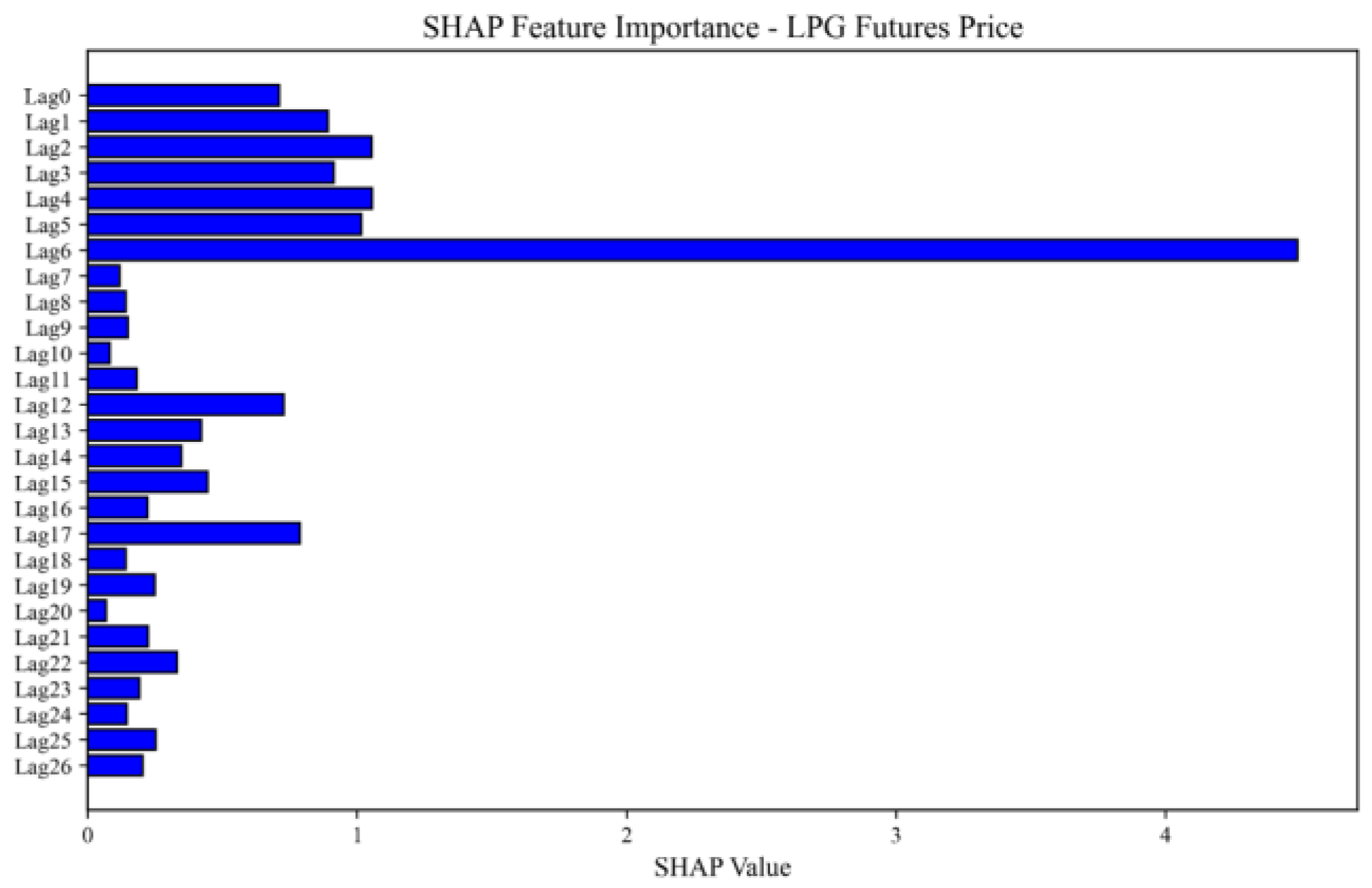
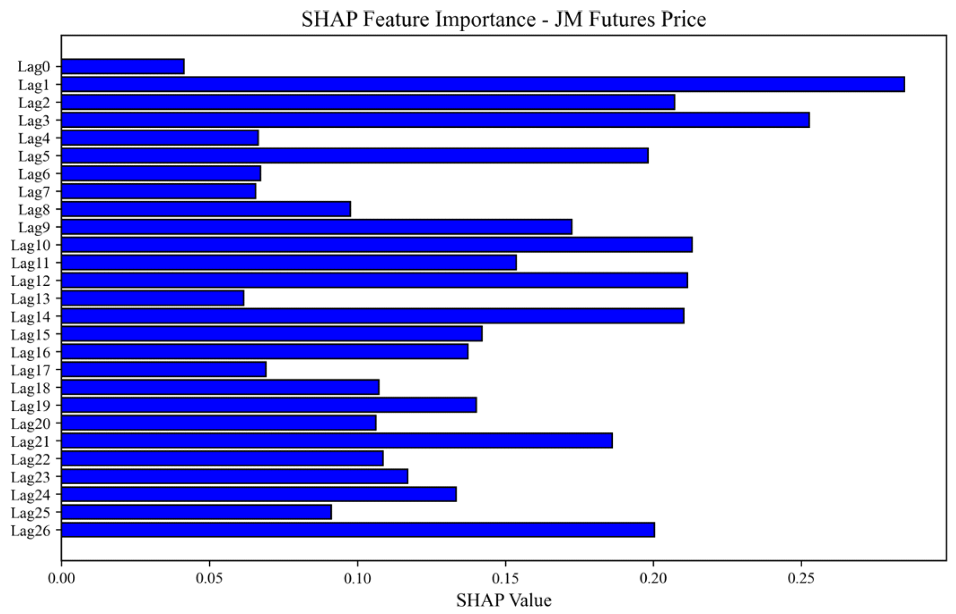
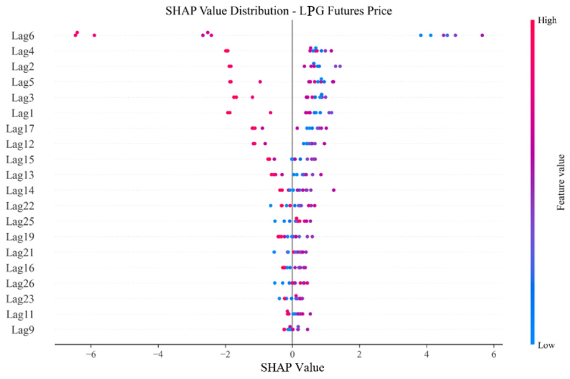
This study applies SHAP value analysis to investigate the lagged influence mechanism of energy futures prices on medium- and long-term electricity prices, based on data from 2023. Figure 8 and Figure 9 display SHAP bar plots illustrating the effects of LPG and JM futures on monthly electricity trading prices, while Figure 10 and Figure 11 offer a more detailed visualization of these effects. In these figures, variables are ranked on the vertical axis from highest to lowest according to their influence on electricity prices. Each point represents an individual observation, with its color and size corresponding to the feature values shown in the legend. The sign of each SHAP value indicates whether the feature has a positive or negative effect on electricity prices. Lag1 through Lag26 denote the influence strength of futures prices from 1 to 26 days earlier on the monthly centralized electricity trading price.

Figure 8. Feature importance analysis of LPG futures.

Figure 8. Feature importance analysis of LPG futures.

Figure 9. Feature importance analysis of JM futures.

Figure 9. Feature importance analysis of JM futures.

Figure 10. Explainability analysis of LPG futures.

Figure 10. Explainability analysis of LPG futures.

Figure 11. Explainability analysis of JM futures.

Figure 11. Explainability analysis of JM futures.

The SHAP value analysis of LPG futures prices reveals a distinct concentration trend characterized by a unimodal decay pattern. The most prominent feature is the futures price from six days before the release of the electricity price, which exhibits significantly greater importance than all other features. This finding suggests that fluctuations in LPG futures prices are strongly transmitted to electricity prices with an approximate six-day lag. Additionally, prices from one to five days earlier also exert a notable influence on electricity price prediction—an effect weaker than that of the sixth day but still considerably stronger than those from other periods. Furthermore, secondary SHAP value peaks appear on the 12th, 17th, and 22nd days before the release date, indicating possible periodic transmission effects. Therefore, it can be inferred that LPG futures prices exert a clear lagged influence on electricity prices, with the strongest impact occurring at approximately a six-day lag.

Further analysis of the decision plot shows that the high-impact red price points are concentrated almost entirely in the negative SHAP value region. This pattern is consistent with the hypothesis that rising natural gas prices may prompt power plants to reduce the share of gas-fired generation and shift to alternative energy sources, thereby temporarily curbing the upward trend in electricity prices. However, this interpretation remains a plausible theoretical explanation rather than an empirically validated conclusion, as actual generation mix data were not incorporated into the model.

The SHAP value analysis of JM futures prices indicates that, compared with LPG futures, JM futures exert a lower overall influence on electricity prices. The SHAP values across different lag periods are more evenly distributed but still display a distinct cyclical pattern.

In the short term, JM futures prices from one to three days before the release of electricity prices show a relatively strong influence, suggesting that short-term fluctuations in coal prices are rapidly transmitted to the electricity market. These price signals directly shape market participants’ expectations and are quickly reflected in electricity price movements. In the medium term, the influence of JM futures prices peaks between days ten and fourteen, exhibiting a distinct cyclical pattern. This suggests that electricity prices are significantly influenced by factors such as power plant inventory management, coal procurement strategies, and transportation cycles. In the long term, coking coal prices from days twenty-one to twenty-six continue to exert a measurable influence on electricity prices, further confirming the presence of long-term cyclical effects.

Further analysis of the SHAP decision plot reveals that the relationship between JM futures prices and electricity prices varies across time scales. In the short term, this relationship is negative, suggesting that rising coking coal prices may suppress electricity demand and thus place downward pressure on short-term electricity prices. However, in the medium and long term, the relationship turns consistently positive. This pattern aligns with the cost transmission mechanism hypothesis of coking coal as a primary fuel for power generation, where higher coking coal prices raise fuel costs and, in turn, drive up electricity prices. It should be noted that the strength and immediacy of this transmission may be moderated by factors such as power plant inventories and long-term contracts, which were not directly modeled in this study.

The above analysis demonstrates that the relationship between JM futures prices and electricity prices varies markedly across time scales, showing a distinct shift from negative to positive in the medium and long term. Among these, the SHAP values in the medium term are more concentrated and display stronger and more stable correlations. Therefore, the medium-term time frame should be regarded as the primary focus for developing coking coal futures trading strategies.

These observed correlations can be interpreted in light of energy structure theory. For coking coal, as a primary baseload energy source, the positive correlation with electricity prices may stem from the fact that increases in its price directly raise fuel costs and, consequently, drive up electricity prices. In contrast, natural gas primarily serves as a supplementary energy source for peak shaving [25]. A plausible speculation is that when natural gas prices rise, power generation companies may reduce its usage, leading to a substitution effect that could suppress marginal demand and limit electricity price increases. This might explain the observed negative correlation between natural gas prices and electricity prices. It should be emphasized that the above mechanisms are inferences based on economic theory and market, and future empirical validation using micro-level data on unit output and fuel switching is warranted.

3.3. Robustness and Quantitative Analysis of SHAP Results

To comprehensively assess the robustness of the SHAP analysis results and gain an in-depth understanding of the interaction mechanisms among lagged variables, this section conducts supplementary analyses in three dimensions: first, verifying the stability of SHAP values for key lagged terms via Bootstrap resampling; second, calculating the cumulative SHAP contributions across different time scales using a window aggregation approach; and finally, discussing the impact of collinearity among lagged variables on SHAP interpretation and the corresponding mitigation strategies.

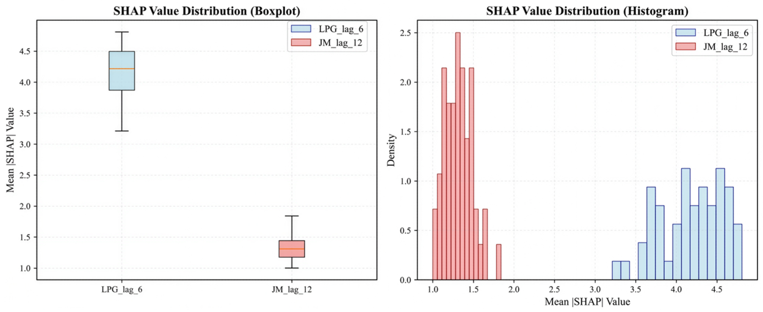
Given the potential high correlation among lagged variables, which may affect the stability of SHAP value estimation, this study adopts the Bootstrap resampling method to perform 50 rounds of sampling with replacement on the training dataset. For each resampling iteration, the random forest model is retrained and SHAP values are recalculated. Particular attention is paid to two key lagged terms: LPG futures lagged by 6 days and JM futures lagged by 12 days. To balance computational efficiency and statistical reliability, each Bootstrap iteration uses 50 randomly selected samples for SHAP value calculation.

The stability test results are shown in Figure 12, with key statistics summarized in

Table 2. Results of Bootstrap Stability Tests for Key Lagged Terms.

Lagged Term	Mean	Standard Deviation	CV	95% Confidence Interval	Sample Size (N)
LPG_lag_6	4.185	0.386	0.092	[3.211, 4.808]	50
JM_lag_12	1.319	0.172	0.131	[1.001, 1.841]	50

Note: Coefficient of Variation (CV) = Standard Deviation/Mean. A CV < 0.15 indicates good stability.

. For LPG_lag_6, the distribution of the mean absolute SHAP values across 50 Bootstrap iterations ranges from [3.21, 4.81], with a mean of 4.18, a standard deviation of 0.39, and a coefficient of variation (CV) of 0.092. For JM_lag_12, the mean SHAP value distribution ranges from [1.00, 1.84], with a mean of 1.32, a standard deviation of 0.17, and a coefficient of variation of 0.131. The coefficients of variation for both key lagged terms are below 0.15, indicating good stability of the SHAP values across Bootstrap resampling. Notably, the signs of the SHAP values remain consistent across all Bootstrap samples, further confirming the reliability of the direction of influence.

To overcome the limitations that single lag-point estimates may be affected by random fluctuations and to systematically evaluate the cumulative impact of futures prices across different time scales, this study further calculates the sum of absolute SHAP values for all lagged terms within short-, medium-, and long-term time windows. The time windows are divided as follows: short-term (lagged 1–7 days), medium-term (lagged 8–14 days), and long-term (lagged 15–26 days). The window aggregation approach effectively smooths out random fluctuations of individual lagged terms and provides a more robust assessment of impact across time scales.

To address the limitations of single-lag point estimates, which may be influenced by random fluctuations, and to systematically assess the cumulative impact of futures prices across different time scales, this study further calculates the sum of the absolute SHAP values of all lag terms within short-, medium-, and long-term time windows. The time windows are divided as follows: short-term (lags 1–7 days), medium-term (lags 8–14 days), and long-term (lags 15–26 days). The window aggregation method effectively smooths random fluctuations in individual lag terms, providing a more robust evaluation of impacts across time scales.

Table 3. Cumulative SHAP Contributions of Futures Prices across Different Time Windows.

Futures Contract	Time Window	Lag Range	Cumulative Absolute SHAP Value	Relative Contribution (%)
LPG	Short-term	1–7 days	9.541	64.20%
LPG	Medium-term	8–14 days	2.053	13.81%
LPG	Long-term	15–26 days	3.268	21.99%
JM	Short-term	1–7 days	1.142	30.05%
JM	Medium-term	8–14 days	1.539	40.48%
JM	Long-term	15–26 days	1.120	29.47%

presents the cumulative SHAP contributions of LPG and JM futures across different time windows. The results show that the impact of LPG futures is highly concentrated in the short-term window, with its short-term cumulative SHAP contribution accounting for 64.2% of the total. The peak occurs at lag 6 days, which aligns with the rapid price signal transmission characteristics of LPG as a peaking energy source. In contrast, the impact of JM futures is more evenly distributed across all windows, with the medium-term window contributing 40.5%, making it the most influential period. The peak occurs at lag 12 days, reflecting the longer inventory and procurement cycles required for the transmission of basic fuel costs. This differentiated impact pattern across time scales provides a quantitative basis for designing differentiated hedging timing strategies.

It should be emphasized that the objective of the SHAP analysis in this study is not to precisely estimate the independent coefficients of each lag term, but rather to identify the historical time windows that have the most significant influence on future electricity price predictions from the perspective of the forecasting model. Therefore, key lag points such as “Day 6” and “Day 12” revealed by SHAP values should be understood as the historical information windows that the model most relies on to make reliable predictions. The window aggregation analysis further validates the robustness of these key windows. This shift in methodological perspective allows the study to extract robust and actionable hedging signals from highly collinear lag variables, perfectly aligning with the closed-loop design objectives from prediction to strategy execution.

In summary, through Bootstrap stability testing, quantitative window aggregation, and an in-depth discussion of collinearity issues, the supplementary analysis in this section systematically verifies the robustness of the SHAP results and provides a cross-temporal quantitative impact assessment. This establishes a reliable methodological foundation for the subsequent differentiated design of hedging strategies.

3.4. Futures Market Hedging Strategy Design

SHAP value analysis reveals a significant correlation between LPG and JM futures prices and monthly electricity trading prices. Specifically, when LPG futures prices decline, monthly electricity trading prices typically increase after an approximately six-day transmission lag. In contrast, when JM futures prices rise, monthly electricity trading prices generally increase after around a twelve-day transmission lag, and vice versa.

These findings further suggest that fluctuations in LPG and JM futures prices can serve as effective predictors of electricity price changes. In particular, during periods of pronounced price volatility, trends in the futures market can anticipate movements in electricity prices.

Based on these market observations, a position-opening strategy can be designed. The strategy leverages anticipated electricity price fluctuations to guide trading operations in futures commodities, thereby hedging against risks arising from electricity price volatility in the futures market. Specifically, when electricity prices are expected to rise, a long position is taken in LPG futures due to their negative correlation with electricity prices. In contrast, a short position is initiated in JM futures, reflecting their positive correlation. Conversely, when electricity prices are expected to decline, short positions are taken in LPG futures, while long positions are adopted in coking coal futures. Lag analysis identifies the optimal entry points as the sixth trading day before month-end for LPG futures and the twelfth trading day before month-end for JM futures. All positions are systematically closed on the last trading day of the month, coinciding with the official publication of monthly electricity trading prices.

4. Optimal Portfolio Risk Optimization Using t-GARCH and Monte Carlo CVaR

4.1. CVaR Calculation Methodology

Value at Risk (VaR) is a quantitative measure used to assess the risk exposure of a commodity portfolio [25]. VaR represents the maximum potential loss of a commodity portfolio at a given confidence level. Specifically, it corresponds to the 1 − α quantile in the lower tail of the loss distribution. For example, if a portfolio is held for one day and the confidence level is 95%, a VaR value of 100 means there is only a 5% chance that the portfolio will lose more than 100 in one day. A higher VaR value indicates a greater level of risk faced by the portfolio. The main drawback of VaR lies in its failure to measure the severity of tail losses: VaR only provides a loss threshold corresponding to the probability of 1 − α, but does not reveal the average magnitude of losses when they exceed this threshold (i.e., fall into the extreme tail of the distribution). It cannot distinguish between thin-tailed and fat-tailed distributions. Therefore, in this study, to comprehensively assess risk, we not only calculate VaR but also compute its complementary metric—Conditional Value at Risk (CVaR). CVaR measures the average level of losses when they exceed the VaR threshold, effectively capturing tail risk. It is primarily determined by market volatility and a given confidence level.

$$B_{\mathrm{CVaR}}=B_{\mathrm{VaR}}+{\displaystyle \frac{1}{n(1-\beta )}}\sum _{n=1}^N\max [0,L_n-B_{\mathrm{VaR}}]$$

(15)

In Equation (15); $B_{\mathrm{VaR}}$ denotes the maximum potential loss of the portfolio; $\beta$ indicates the given confidence level.

In this study, the Monte Carlo simulation method is used to generate a large number of random sample paths to simulate the price movements over the next 30 days. For each path, the corresponding loss value is calculated. Based on the distribution of losses across all simulated paths, the CVaR at a specified confidence level is computed. This result is then used to determine the optimal weight allocation between the two futures.

4.2. Comparing Normal and t-GARCH CVaR Models for Optimal Allocation

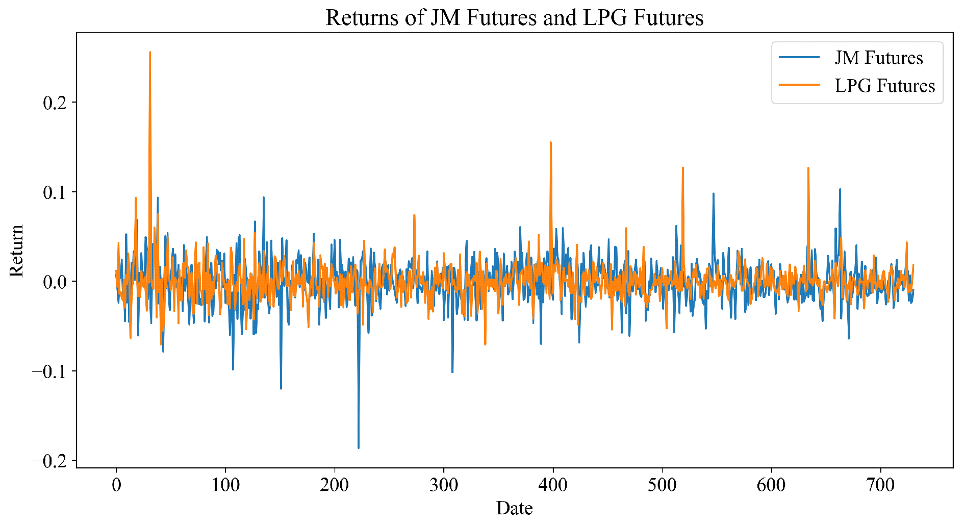
In financial derivatives risk management, the distribution characteristics and volatility structure of return series directly determine a model’s ability to capture extreme risks. Traditional approaches assume that residuals are independent and identically distributed with constant variance, which contradicts common features of financial time series such as volatility clustering and heavy tails. To more thoroughly characterize the differences in return properties and tail risks among energy commodities, this study conducts statistical feature analysis, distribution fitting tests, and GARCH model estimation for the return series of JM futures and LPG futures. Furthermore, volatility models under normal and t-distribution assumptions are used to calculate CVaR at different confidence levels. All analyses are based on 731 daily return samples, with risk values computed using Monte Carlo simulation with 5000 iterations, a 30-day time step, and 1000 weight search points, ensuring numerical stability and statistical significance. The historical returns of the two commodities are illustrated in Figure 13.

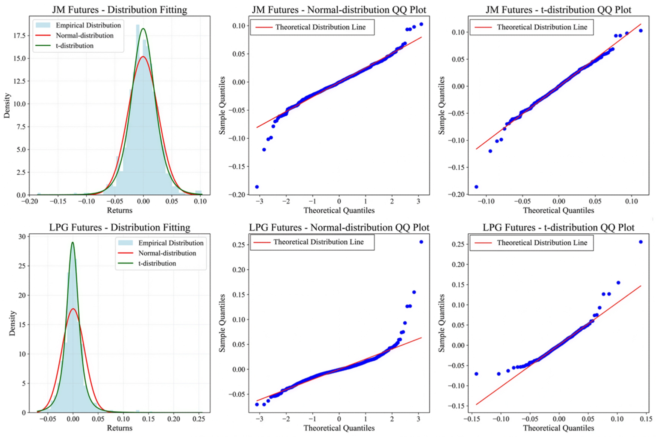
As shown in Figure 14, the returns of JM futures have a mean of −0.000692 and a standard deviation of 0.026268, exhibiting slight negative skewness (−0.5065) and a kurtosis of 4.6160, which exceeds the normal distribution benchmark of 3, indicating a heavy-tailed distribution and significant deviation from normality. In contrast, the returns of LPG futures have a mean of 0.000121 and a standard deviation of 0.022541, but display pronounced positive skewness (2.9631) and extreme kurtosis (27.9319), reflecting strong right-skewness and leptokurtic behavior, likewise significantly rejecting the normality assumption.

The probability density fitting of the sample returns indicates that the normal distribution, due to its lower kurtosis and rapidly decaying tails, fails to adequately capture the occurrence probability of extreme returns. In contrast, the t-distribution exhibits higher probability density in the tail regions, reflecting pronounced heavy-tailed behavior. These results suggest that the returns of both energy futures exhibit asymmetry and fat tails, with LPG futures showing more pronounced volatility and a significantly higher frequency of extreme fluctuations compared to JM futures.

To further characterize the tail structure, the returns were fitted using the t-distribution. The estimated degrees of freedom are 5.7499 for JM futures and 2.8583 for LPG futures, indicating that LPG futures have heavier tails and a higher likelihood of extreme price movements during periods of market turbulence, resulting in greater risk exposure compared to JM futures. This finding is consistent with the probability density fitting curves in Figure 14, where the t-distribution provides a superior fit to extreme returns in the tail regions compared to the normal distribution. The Q-Q plots further confirm these differences: under the normality assumption, sample points, particularly in the left tail, deviate noticeably below the diagonal, indicating that the actual probability of extreme losses exceeds the prediction of the normal distribution. In contrast, the Q-Q plot for the t-distribution closely aligns with the theoretical quantile line, with only minor deviations at the extreme tails, demonstrating its superior suitability for capturing tail risks.

This distributional difference arises from the degrees of freedom parameter $\nu$ introduced in the t-distribution, which allows flexible characterization of extreme risks by adjusting tail thickness. When $\nu \to \infty$, the t-distribution approaches the normal distribution; conversely, when $\nu$ are small, the tails become heavier, effectively capturing atypical fluctuations commonly observed in financial data. For a return series $r_t$ under a GARCH conditional heteroskedasticity framework, the model can be expressed as:

$$r_t=\mu +{\epsilon }_t,{\epsilon }_t={\sigma }_t{z}_t,{\sigma }_t^2={\alpha }_0+{\alpha }_1{s}_{t-1}^2+{\beta }_1{\sigma }_{t-1}^2$$

(16)

Here, $z_t$ follows different distributional assumptions depending on the model: if ${\mathrm{z}}_{\mathrm{t}}\sim \mathrm{N}\left(\mathrm{0,1}\right)$, it corresponds to a normal GARCH model; if $z_t\sim t_{\nu }(0,1)$, it corresponds to a t-GARCH model.

Based on

Table 4. Results of Significance Tests.

Parameter	JM Futures	LPG Futures
Mean Constant	−0.000831	−0.000965
Variance Constant (ω)	3.10 × 10−5	7.60 × 10−7
ARCH Term (α)	0.0451 ***	0.0000
GARCH Term (β)	0.9079 ***	0.9956 ***
Degrees of Freedom (ν)	6.014 ***	3.158 ***
α + β	0.9530	0.9956

Note: *** denote significance at the 1% levels.

, a GARCH (1,1) model with a t-distribution was employed to model the conditional volatility of the two futures contracts. This specification is particularly well-suited to accommodate the pronounced leptokurtosis and heavy tails observed in the data, which deviate significantly from normality as illustrated in Figure 14. For JM futures, the estimated results yield a mean equation constant of −0.00083109 and a variance constant of 0.00003095. The ARCH parameter α is 0.045099, while the GARCH parameter β reaches 0.907946, with degrees of freedom approximately 6.0138. The β value close to 1 indicates substantial volatility persistence, implying that current market volatility is strongly conditioned by its past values.

In contrast, the estimation for LPG futures reveals a distinct volatility structure where the ARCH coefficient becomes statistically insignificant (near zero), while the GARCH parameter reaches 0.995647. This suggests that LPG futures’ volatility responds weakly to transitory short-term shocks, which are instead rapidly absorbed into the long-term volatility component. Such behavior is consistent with markets characterized by infrequent but substantial price jumps, where volatility responds more through persistent structural components rather than immediate noise. Furthermore, the sum of ARCH and GARCH coefficients for LPG futures is nearly unity, suggesting near-integrated volatility dynamics. This reflects the strong volatility clustering and long-memory effects commonly observed in energy commodity markets, where the impact of market shocks tends to persist over extended horizons.

The use of the t-distribution substantially improves the overall fit by capturing the extreme tail behavior of LPG returns, which exhibit a low degree of freedom at 3.1580, indicating the presence of rare but large price movements. Although more flexible specifications such as EGARCH and GJR-GARCH are capable of capturing potential asymmetry, the standard GARCH model with Student’s t-innovations is maintained as the baseline to ensure interpretability and direct comparability between the JM and LPG contracts.

4.3. Determination of Commodity Weights

As shown in Figure 15, the CVaR comparison curves indicate that CVaR increases with higher confidence levels under different distributional assumptions, reflecting that stricter risk control requires the model to allocate larger buffers for potential extreme losses. Under the t-GARCH model, the portfolio CVaR at the 90%, 95%, and 99% confidence levels are 0.17797, 0.20524, and 0.25869, respectively, with corresponding weights for JM and LPG futures of (0.449, 0.551), (0.416, 0.584), and (0.387, 0.613). This suggests that at low to medium confidence levels, the model favors a higher allocation to LPG to mitigate the high volatility risk of JM futures, whereas at high confidence levels, the weight of JM futures increases, indicating its relatively lower risk contribution under extreme scenarios.

Compared to the normality assumption, the t-GARCH model generally produces higher risk estimates, particularly at high confidence levels, indicating that the t-distribution assumption better captures the risk of extreme events. Regarding portfolio weights, the allocation to JM futures under the t-distribution model is noticeably higher than under the normal model, suggesting that the model recognizes the right-skewed and extreme volatility characteristics of LPG returns and consequently reduces its weight in the optimization to mitigate potential risk.

Based on the results above, the normal distribution assumption provides relatively smooth risk estimates under moderate risk conditions but has limited capability to capture tail risks, often underestimating the probability of extreme losses. In contrast, the t-distribution model, through its degrees of freedom parameter, relaxes tail assumptions and more accurately characterizes abnormal market fluctuations at high confidence levels. In the energy futures market, prices are influenced by multiple factors such as supply and demand, seasonality, and geopolitical events, resulting in highly asymmetric and abrupt volatility. Therefore, employing a GARCH model under the t-distribution assumption significantly enhances the reliability of risk assessment. Considering both return and risk, this study adopts the portfolio weights calculated under the 95% confidence level t-GARCH model, with JM and LPG futures allocated at 0.416 and 0.584, respectively.

This result indicates that the diversified portfolio offers effective risk hedging. With this asset allocation, risk can be effectively diversified, reducing potential losses and providing strong data support for optimizing asset allocation and developing safer hedging strategies.

5. Case Study Analysis

5.1. Experimental Environment and Parameter Settings

All experiments in this study were conducted on a high-performance mobile workstation equipped with an AMD Ryzen 9 7945HX processor (16 cores, 32 threads, base frequency 2.50 GHz) and an NVIDIA GeForce RTX 4060 Laptop GPU (8 GB GDDR6 memory). The system was configured with 16 GB DDR5 RAM and ran a 64-bit Windows operating system. All model development and experiments were performed in a Python 3.11.3 environment, using TensorFlow and Keras as the primary frameworks for building and training the LSTM model. Data processing was implemented with Pandas and NumPy, normalization was performed using the MinMaxScaler module from scikit-learn, and visualization was achieved through Matplotlib 3.8.3.

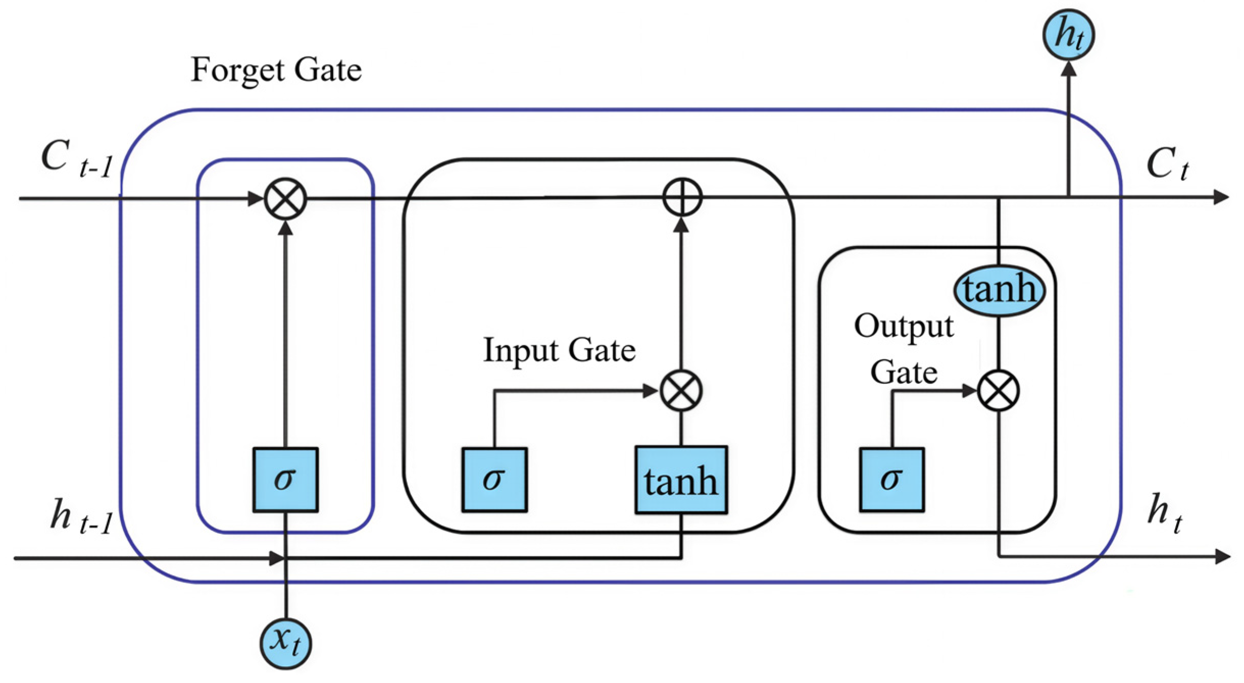
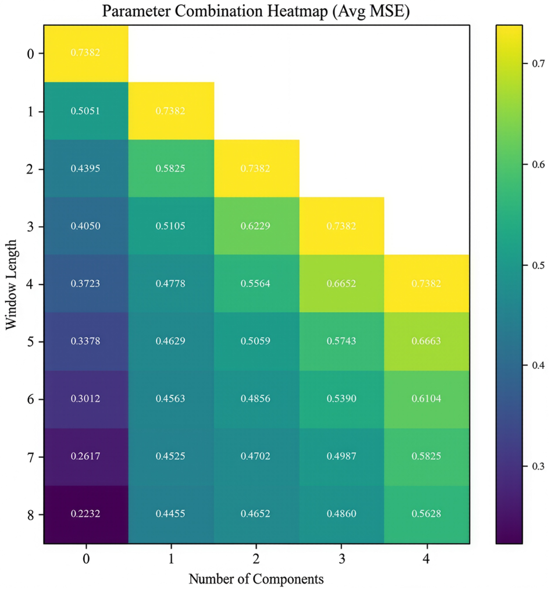
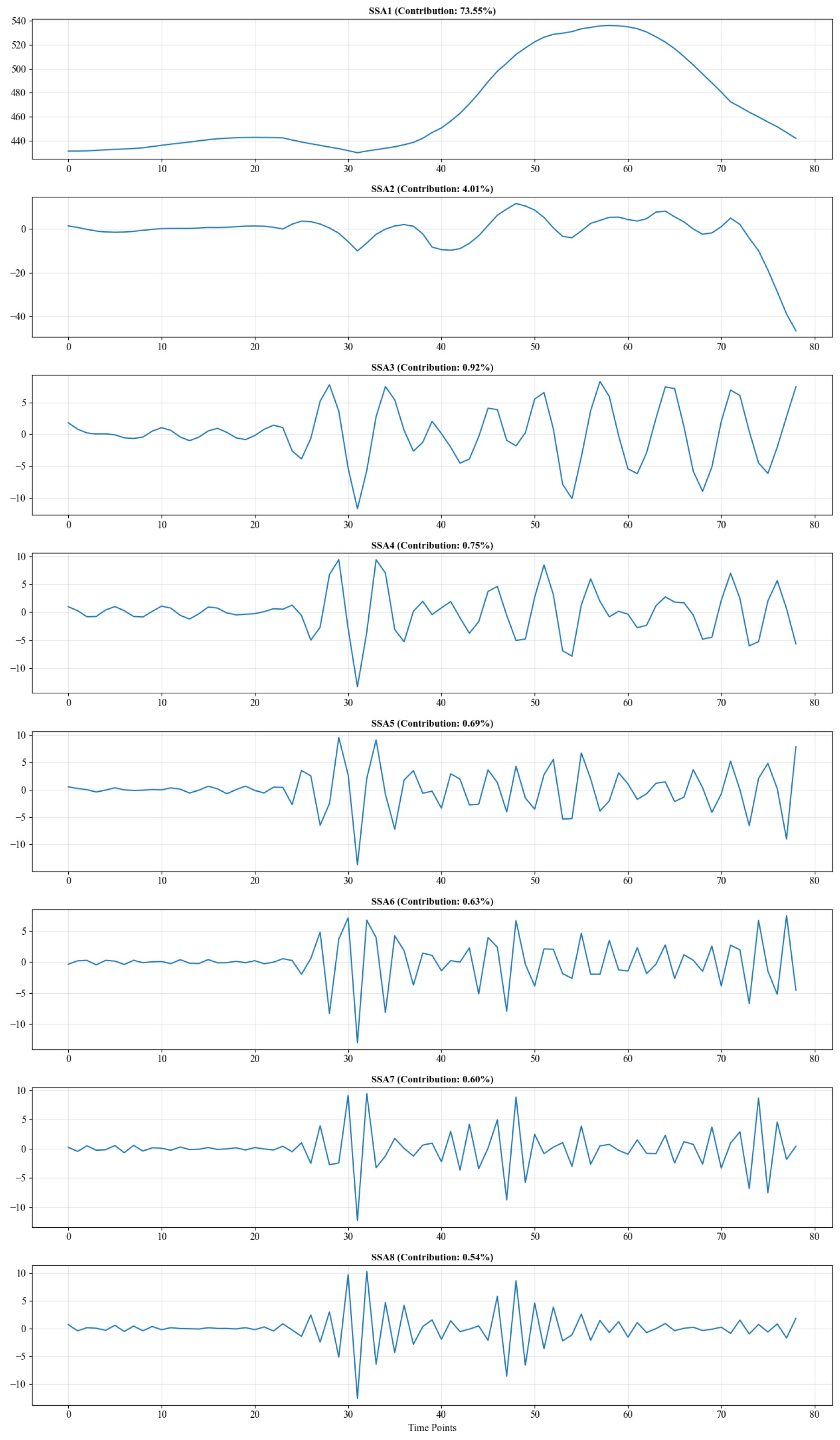
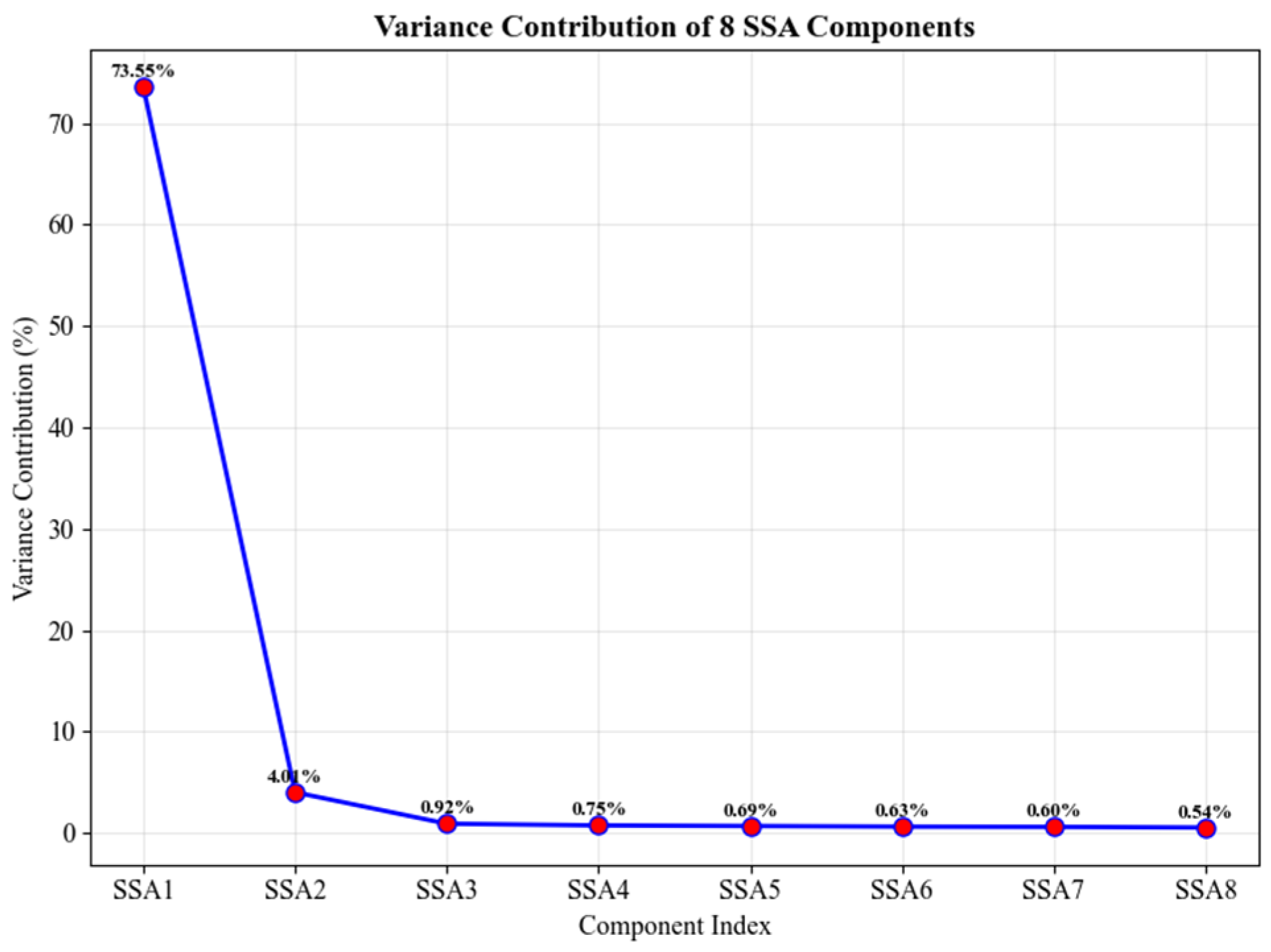
In the SSA-LSTM hybrid electricity price forecasting model of this study, the first two SSA components were recombined into a low-frequency trend component based on singular value contribution analysis, while the remaining six components were recombined into high-frequency fluctuation components. The LSTM network was configured as a two-layer architecture: the first layer contains 100 neurons to capture long-term dependencies, and the second layer contains 50 neurons to learn local features. A dropout rate of 0.3 was applied to prevent overfitting. The model was trained to predict future electricity prices using historical data with a time step of 3. Data were normalized to the [0, 1] range using MinMaxScaler. For optimization, RMSprop was used for the low-frequency component to ensure stable convergence, while Adam was applied to the high-frequency components to quickly adapt to fluctuations. The training process used a batch size of 20 and 20 epochs, with the mean squared error (MSE) as the loss function. The dataset was split chronologically, reserving the last 12 samples as the test set.

5.2. Analysis of Forecast Results of Electricity Prices

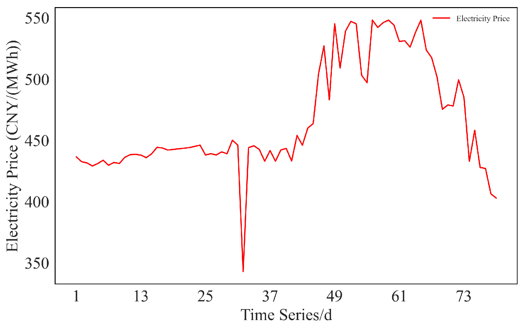
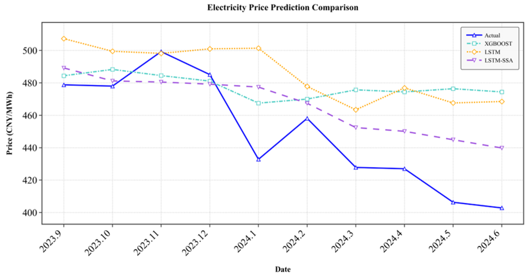
This study performs a case analysis from the perspective of the electricity retailer in Guangdong’s electricity market, using the SSA-LSTM model to predict monthly trading electricity prices in the Guangdong electricity market. The dataset from January 2018 to August 2023 is used for training, with a one-step prediction model and rolling training method applied. Monthly trading electricity prices from September 2023 to June 2024 are forecasted, and an energy futures strategy will be developed in the first half of 2024 to hedge against fluctuations in electricity procurement costs. The electricity price prediction results are shown in

Table 5. Electricity Price Prediction Results and Actual Values.

Date	Actual	XGBOOST	LSTM	LSTM-SSA
2023.09	478.8	484.4	507.3	489.2
2023.10	478	488.3	499.5	481.2
2023.11	499.3	484.5	498.2	480.5
2023.12	485.1	481.1	501.0	479.2
2024.01	432.8	467.5	501.4	477.4
2024.02	458.1	470.0	477.8	467.4
2024.03	427.8	475.7	463.4	452.4
2024.04	427	474.4	476.9	450.1
2024.05	406.3	476.4	467.6	444.9
2024.06	402.8	474.4	468.5	439.8

, and the evaluation results are presented in

Table 6. Model Evaluation Metrics.

Date	XGBOOST	LSTM	LSTM-SSA
2023.09	5.6	28.5	15
2023.10	10.3	21.5	8.2
2023.11	−14.8	−1.1	−12.1
2023.12	−4	15.9	3.3
2024.01	34.7	68.6	53.4
2024.02	11.9	19.7	16.9
2024.03	47.9	35.6	31.1
2024.04	47.4	49.9	26.8
2024.05	70.1	61.3	37.8
2024.06	71.6	65.7	35.7
RMSE	40.37	42.96	28.24
MAPE	7.51%	8.55%	5.00%
MAE	31.83	36.78	21.55

. The specific trend is shown in Figure 16.

To better evaluate the prediction results and make further adjustments to the model parameters, the Root Mean Squared Error (RMSE), Mean Absolute Percentage Error (MAPE) and Mean Absolute Error (MAE) are selected as evaluation metrics, with their mathematical expressions given by:

$$RMSE=\sqrt{{\displaystyle \frac{1}{n}}\sum _{i=1}^n{({\hat{\mathrm{y}}}_i-{\mathrm{y}}_i)}^2}$$

(17)

$$MAPE={\displaystyle \frac{100\%}{n}}\sum _{i=1}^n\left|{\displaystyle \frac{{\hat{\mathrm{y}}}_i-{\mathrm{y}}_i}{{\mathrm{y}}_i}}\right|$$

(18)

$$MAE={\displaystyle \frac{1}{n}}\sum _{i=1}^n\left|{\hat{\mathrm{y}}}_i-{\mathrm{y}}_i\right|$$

(19)

In Equations (17)–(19), n denotes the sample size; ${\hat{\mathrm{y}}}_i$ represents the predicted electricity price for the i-th sample, ${\mathrm{y}}_i$ denotes the true electricity price for the i-th sample.

Table 6 shows that when electricity prices exhibit significant volatility, the predictions of the XGBOOST, and basic LSTM models generally deviate substantially from the actual values, indicating that they fail to adequately capture and respond to price trends. In reality, electricity prices are influenced by multiple complex factors interacting nonlinearly, and the time series contains abundant nonlinear characteristics. Linear models cannot capture such complex dynamics, resulting in inherently insufficient predictive performance. Moreover, prediction errors tend to accumulate rapidly as the forecasting horizon extends. While the XGBOOST model exhibits relatively small errors at the beginning of the prediction period, the discrepancy between predicted and actual values increases over time, reaching an absolute deviation of 71.6 by June 2024.

In contrast, the superior performance of the LSTM-SSA model stems from its successful mitigation of the aforementioned limitations through Singular Spectrum Analysis (SSA). The LSTM model learns from a series that has been purified by SSA, in which trend and major periodic components are more pronounced. This allows the LSTM to focus on robust long-term dependencies and core dynamics without being confounded by noise and irrelevant fluctuations. Consequently, the LSTM-SSA predictive trajectory closely tracks the actual price decline, exhibiting minimal systematic bias. Furthermore, all evaluation metrics, including RMSE (28.24), MAPE (5.00%), and MAE (21.55), demonstrate significantly better performance than those of the comparative models.

In summary, the LSTM-SSA model, employing its unique “decompose-learn” framework, effectively overcomes the limitations of traditional models—such as the linearity assumption and rigid handling of seasonality—while enhancing LSTM’s ability to identify true trends amid noise. This framework enables the model to deliver more accurate and reliable electricity price forecasts, providing electricity retailers with greater confidence in decision-making and enhanced risk management capabilities when formulating procurement strategies, estimating expected costs, and designing hedging schemes, compared with other models.

5.3. Trading Strategy

Based on the forecasting results indicating a consistent downtrend in electricity prices from January to June 2024, this study designs a position-opening strategy involving long positions in JM futures and short positions in LPG futures throughout this period.

Table 7. Futures Price.

Date	LPG Futures Position	LPG Futures (CNY/ton)	JM Futures Position	JM Futures (CNY/ton)
2024.01	short positions	Open: 4288 Close: 4352	long positions	Open: 1816.5 Close: 1751
2024.02	short positions	Open: 4233 Close: 4137	long positions	Open: 1647 Close: 1772.5
2024.03	short positions	Open: 4666 Close: 4658	long positions	Open: 1638.5 Close: 1471.5
2024.04	short positions	Open: 4631 Close: 4556	long positions	Open: 1791.5 Close: 1806
2024.05	short positions	Open: 4664 Close: 4778	long positions	Open: 1724.5 Close: 1679.5
2024.06	short positions	Open: 4726 Close: 4705	long positions	Open: 1616 Close: 1603

shows the futures prices and

Table 8. Volatility of Electricity Prices and Futures Prices.

Date	Electricity Price Change Rate	JM Futures Volatility	LPG Futures Volatility
2024.01	−10.78%	−3.606%	1.493%
2024.02	5.85%	7.620%	−2.268%
2024.03	−6.61%	−10.192%	−0.171%
2024.04	−0.19%	0.809%	−1.620%
2024.05	−4.85%	−2.609%	2.444%
2024.06	−0.86%	−0.804%	−0.444%

shows their volatility.

According to the analysis in Table 8, the futures trading strategy closely aligns with market price fluctuations. The correlation coefficient between JM futures price volatility and electricity price volatility is 0.82, while the correlation coefficient between LPG futures price volatility and electricity price volatility is −0.79. The correlation between futures price volatility and electricity price volatility when combined by weights is 0.89. In the Monte Carlo simulation, the correlation between the return series of JM futures and LPG futures is set based on the sample historical correlation coefficient and is assumed to remain constant during the simulation period. While this approach captures the static linear dependence between the two assets, it does not reflect potentially time-varying correlation structures. Future research could consider introducing dynamic conditional correlation models (e.g., DCC-GARCH) to further investigate the impact of changing correlation structures on portfolio risk.

5.4. Hedging and Return Analysis

This study uses the Guangdong electricity market as a case for validation, with the actual electricity purchase cost calculated based on the market average. Futures market operations follow the strategy outlined in

Table 9. Electricity Purchase and Futures Costs.

Date	Electricity Purchase (104 CNY)	JM Futures (104 CNY)	LPG Futures (104 CNY)	JM Contracts	LPG Contracts
2024.01	156.06	74.01	103.90	+7	−12
2024.02	140.95	66.84	93.84	+7	−11
2024.03	250.92	119.00	167.05	+12	−18
2024.04	156.02	74.00	103.87	+7	−11
2024.05	183.62	87.08	122.25	+8	−13
2024.06	110.38	52.35	73.49	+5	−8

, with investment amounts for LPG and JM futures allocated according to the results of the CVaR calculation.

Based on the electricity purchase cost, different proportions of capital are invested in the futures market for hedging, results are shown in Figure 17. Within the hedging ratio range of 0% to 200%, it can be observed that as the hedging ratio increases, the total return of the strategy gradually declines.

Risk indicator analysis shows that, at low hedging ratios, both volatility and drawdown are relatively high. As the hedging ratio increases, risk gradually decreases until reaching a minimum, after which it begins to rise again.

The Sharpe ratio exhibits a “mountain-shaped” curve, peaking at a hedging ratio of 127%, indicating that the strategy achieves an optimal allocation by balancing return and risk. This represents the most efficient configuration in terms of risk-adjusted performance.

Table 9 shows the electricity purchase cost and the monthly investment in the futures market. In the ‘JM Contracts’ and ‘LPG Contracts’ columns, ‘+’ indicates long positions, while ‘−’ denotes short positions. Since futures contracts can only be traded in whole lots, which are 60 tons per lot for JM futures and 20 tons per lot for LPG futures, the nearest rounding method is applied during the calculation.

The rise in monthly electricity trading prices leads to an increase in electricity purchase costs, thereby reducing the profit. Based on the purchase amounts in Table 6, the corresponding returns are shown in

Table 10. Monthly Returns.

Date	Electricity Revenue (104 CNY)	JM Futures Only (104 CNY)	LPG Futures Only (104 CNY)	Portfolio Hedging (104 CNY)
2024.01	16.83	11.33	14.53	12.61
2024.02	−8.24	2.30	−4.98	−1.02
2024.03	16.60	−9.45	17.03	4.76
2024.04	0.29	1.59	2.84	2.57
2024.05	8.90	4.04	4.34	3.64
2024.06	0.95	0.09	1.45	0.85

and

Table 11. Profitability Analysis.

	Electricity Revenue (104 CNY)	JM Futures Only (104 CNY)	LPG Futures Only (104 CNY)	Portfolio Hedging (104 CNY)
Total	35.33	9.90	35.22	23.41
Average	5.89	1.65	5.87	3.90
Volatility	9.12	6.13	7.62	4.73
MDD	8.24	9.45	4.98	1.02
Sharpe ratio	2.04	0.85	2.43	2.86

.

Based on the data analysis for the first half of 2024, the portfolio hedging strategy demonstrates multidimensional advantages in electricity cost risk management:

(1)

Regarding return performance, the LPG hedging strategy achieves the highest total return (352,200 CNY) and average return (58,700 CNY), indicating strong profitability. However, these returns are accompanied by relatively high volatility (7.62) and a maximum drawdown of −49,800 CNY, suggesting that although the returns are substantial, the associated risks remain considerable.

(2)

The JM hedging strategy performed the poorest, exhibiting both the lowest total return (99,000 CNY) and the largest maximum drawdown (−94,500 CNY), making it the riskiest strategy. Moreover, its Sharpe ratio is only 0.85, indicating relatively low return efficiency per unit of risk.

(3)

The combined hedging strategy exhibits a clear overall advantage across multiple performance indicators. Its total return of 234,100 CNY, though lower than that of the LPG strategy, is accompanied by the lowest volatility (4.73) and a maximum drawdown of only −10,200 CNY, resulting in minimal significant losses. Furthermore, its Sharpe ratio of 2.86—the highest among the three strategies—indicates that the combined strategy excels in stability and risk control, offering strong risk-adjusted return potential.

(4)

Based on

Table 12. Risk-Return of Different Prediction Models.

	Volatility	MDD	Sharpe Ratio
XGBOOST	16.78	16.91	1.57
LSTM	8.76	1.97	1.65
LSTM-SSA	4.73	1.02	2.86

, the LSTM-SSA model demonstrates the best performance. It achieves the highest Sharpe Ratio (2.86) while maintaining the lowest volatility (4.73) and the smallest maximum drawdown (1.02), reflecting exceptional risk control capabilities and superior risk-adjusted returns. In comparison, XGBOOST carries excessive risk with the lowest return efficiency, and although LSTM outperforms XGBOOST, it is significantly inferior to LSTM-SSA across all metrics.

Empirical analysis indicates that the portfolio hedging strategy preserves most returns during months of positive cost fluctuations while effectively mitigating risks during months of negative fluctuations (e.g., February 2024). This dynamic balancing mechanism renders it an optimized approach for electricity cost management.

6. Discussion

This study, set against the backdrop of electricity market liberalization, addresses the risk posed by electricity price fluctuations in medium- and long-term trading. From the perspective of electricity retailers, using electricity price forecasting as a method, it analyzes the interaction between energy futures and monthly trading electricity prices. The study employs CVaR as a risk assessment metric and develops a model for risk hedging using commodity portfolio trading. The simulation examples are based on real operational data from the electricity market and yield the following conclusions:

(1)

The proposed SSA-LSTM hybrid forecasting framework demonstrates superior performance in capturing nonlinear electricity price patterns, achieving a 34% error reduction compared to conventional models after SSA optimization. This enhanced prediction accuracy provides reliable guidance for formulating futures market strategies.

(2)

The SHAP-based interpretability analysis reveals distinct transmission mechanisms between different energy futures and electricity prices. JM futures show positive correlation with a 12-day transmission cycle, while LPG futures exhibit negative correlation with a 6-day lag, providing scientific basis for determining optimal hedging timing. Furthermore, the data alignment method used in this study, which employs bilinear interpolation to match daily futures prices with the monthly electricity price, represents a pragmatic choice for constructing the forecasting model’s input features. Future research could explore alternative alignment techniques, such as Mixed Data Sampling (MIDAS) regression or aggregation of futures prices to weekly frequency, to further examine the sensitivity of the identified predictive lag windows to different temporal data treatments.

(3)

The t-GARCH-based CVaR methodology effectively captures the fat-tailed characteristics of energy futures returns, outperforming traditional normal distribution assumptions. Portfolio optimization shows that a 0.416:0.584 allocation between JM and LPG futures achieves optimal risk-return characteristics with a combined correlation of 0.89 against electricity price fluctuations.

(4)

The risk faced by the investment portfolio is related to the weight ratio of the investment. After allocating 127% capital for hedging, the volatility decreased from 9.12% to 4.73% (a 48.14% reduction), while the maximum drawdown dropped from 82.4k CNY to 10.2k CNY (an 87.62% decline). The complete methodology establishes a systematic risk management workflow from price forecasting to strategy execution, offering electricity retailers an integrated solution for addressing price volatility in liberalized electricity markets.

The hedging strategy proposed in this study is primarily constructed based on correlation coefficients and lag effects identified from historical data. While it demonstrates effective risk hedging under normal market conditions, it has not been systematically tested under extreme scenarios (such as sharp fluctuations in energy prices, supply disruptions caused by geopolitical events, and other stress conditions). This is because the current research primarily relies on historical market data and focuses on establishing a complete methodological framework and validating its effectiveness under typical market conditions. Future research will focus on developing a multi-scenario stress testing framework to further verify and optimize the strategy’s robustness and adaptability across different market environments by simulating abnormal conditions such as sudden fuel price spikes and extreme weather events. This will serve as an important supplement to improving electricity retailers’ comprehensive risk management systems.