Short-Term Solar and Wind Power Forecasting Using Machine Learning Algorithms for Microgrid Operation

Abstract

Accurate short-term forecasting of renewable energy sources is essential for stable and efficient microgrid operation. Existing models primarily focus on either solar or wind prediction, often neglecting their combined stochastic behavior within isolated systems. This study presents a comparative evaluation of three machine-learning models—Random Forest, ANN, and LSTM—for short-term solar and wind forecasting in microgrid environments. Historical meteorological data and power generation records are used to train and validate three ML models: Random Forest, Long Short-Term Memory, and Artificial Neural Networks. Each model is optimized to capture nonlinear and rapidly fluctuating weather dynamics. Forecasting performance is quantitatively evaluated using Mean Absolute Error, Root Mean Square Error, and Mean Percentage Error. The predicted values are integrated into a microgrid energy management system to enhance operational decisions such as battery storage scheduling, diesel generator coordination, and load balancing. Among the evaluated models, the ANN achieved the lowest prediction error with an MAE of 64.72 kW on the one-year dataset, outperforming both LSTM and Random Forest. The novelty of this study lies in integrating multi-source data into a unified ML-based predictive framework, enabling improved reliability, reduced fossil fuel usage, and enhanced energy resilience in remote microgrids. This research used Orange 3.40 software and Python 3.12 code for prediction. By enhancing forecasting accuracy, the project seeks to reduce reliance on fossil fuels, lower operational costs, and improve grid stability. Outcomes will provide scalable insights for remote microgrids transitioning to renewables.

1. Introduction

Incorporating clean energy technologies such as photovoltaic systems and wind turbines into localized power networks has become essential for isolated and coastal populations pursuing dependable, environmentally responsible electrical infrastructure. Nevertheless, the variable and uncertain characteristics of sunlight availability and air current velocities create significant obstacles to ensuring network equilibrium and uninterrupted energy delivery [1]. Precise prediction of clean energy production is consequently critical for effective power system operations, optimal resource allocation, and reducing dependence on conventional fuel-based reserve generators.

Due to their capacity to simulate nonlinear and time-dependent behaviors in renewable energy data, machine learning techniques, including ANN, LSTM, and Random Forest, have been increasingly popular in recent years. These models have proven to be more accurate in making predictions than traditional statistical techniques [2]. Nevertheless, most existing studies primarily focus on a single energy source (either solar or wind) and typically assume the availability of complete meteorological data [3]. This creates a research gap in understanding model adaptability under data-scarce conditions and combined resource variability, especially within isolated microgrids where measurement infrastructure may be limited.

A classification system called Random Forest uses the majority vote to improve prediction accuracy by creating several decision trees on various dataset segments [4]. This study’s initial dataset was taken from the Portuguese microgrid forecasting competition. By identifying long-term relationships, the LSTM model, a kind of recurrent neural network, is intended to learn and forecast time series data. The microgrid forecasting dataset from Portugal is used in this study to train the random forest model, which predicts future energy usage [5]. Inspired by the human brain, Artificial Neural Networks are computer models made up of layers of interconnected nodes, or neurons, that use data to identify complex patterns. Their capacity to simulate non-linear interactions makes them popular for applications like image recognition, classification, and regression [6]. Recent literature has reported a wide range of data-driven forecasting approaches for individual renewable resources. For photovoltaic (PV) systems, machine- and deep-learning models such as Random Forest, boosting ensembles, and LSTM networks have been applied to short-term power forecasting using combinations of solar irradiance, ambient temperature, and historical power data. For wind farms and hybrid microgrids, LSTM-based architectures and ensemble methods have been adopted to model highly uncertain meteorological dynamics and to support energy management in islanded systems. Several review papers further highlight the rapid growth of AI-based renewable forecasting and discuss the strengths and weaknesses of different model classes, input features, and error metrics. Table 1 summarizes representative studies in the literature, indicating the type of resource (solar, wind, or hybrid), forecasting horizon, main input variables, and reported accuracy indices such as MAE, RMSE, and MAPE.

Table 1. Representative studies on short-term solar and wind power forecasting using machine-learning models.

Ref.	Resource Type	Forecasting Method	Horizon	Main Input Variables	Reported Performance
[1]	Solar PV	RF, GBM	15 min ahead	GHI, temperature, historical PV power	RMSE, MAPE
[4]	Wind	LSTM	1 h ahead	Wind speed, direction, pressure	MAE, RMSE
[7]	Solar	ANN	1 day ahead	Irradiance, temp, power	MAPE
[8]	Hybrid (PV + wind)	LSTM + ensemble	30 min ahead	Wind speed, irradiance, load	RMSE
[9]	Wind	RF	10 min ahead	Wind speed, hub-height features	MAE
[10]	Solar	Review paper	–	–	Comparative MAPE range

The objective of this work is to assess and compare the forecasting performance of three widely used machine-learning models under identical conditions rather than developing a hybrid or integrated model.

2. Database and Methodology

2.1. Database

This study analyzes a dataset comprising the power load demand of the regional grid supplied by the wind farm, alongside generation data from the specific wind farm, which is correlated with historical meteorological records corresponding to the same time period. Moreover, we collected data for the forecasting from the Competition (2022) on solar generation forecasting. The input data, recorded at 5 min intervals, include photovoltaic (PV) power output along with weather-related parameters such as temperature, wind speed, humidity, and additional relevant factors. Table 2 shows the dataset characteristics, and this dataset consists of electricity produced by solar panels, combined with meteorological data obtained from a local weather station. The total dataset is for four years.

Table 2. Dataset characteristics.

Component/Parameter	Description
Generation Type	Mixed solar PV and wind power
PV plant capacity	1.2–1.5 MW (depending on dataset source)
Wind farm capacity	~4 MW maximum recorded output
Meteorological inputs	Solar irradiance, wind speed, temperature, humidity
Measurement interval	5-min resolution
Data period used	6-month, 1-year, and 3-year continuous intervals
Objective	Short-term (5 min ahead) forecasting for microgrid operations

In this work, the six-month, one-year, and three-year datasets were selected because they represent the longest uninterrupted records available from the measurement sources. While actinometric series spanning 10–20 years are ideal for characterizing long-term solar and wind behavior, such extended datasets are typically not accessible for remote microgrids or recently installed renewable systems. As the aim of this study is short-term forecasting rather than long-term climatological modeling, these intervals allow us to examine how the forecast accuracy changes when the training history is limited, which reflects the data conditions commonly encountered in practical microgrid settings.

2.2. Methodology

In this study, three machine-learning models—Random Forest (RF), Long Short-Term Memory (LSTM), and Artificial Neural Network (ANN)—were developed for short-term renewable power forecasting. Prior to model training, a consistent data preprocessing pipeline was applied. Missing values were removed, and all numerical variables were scaled using Min–Max normalization to ensure stable training across the neural network models. Feature selection was performed by incorporating the key meteorological variables influencing power output, including wind speed, ambient temperature, solar irradiance, humidity, and historical power measurements.

To capture temporal dependencies in the data, a structured lag framework was applied. The input sequences included 56 historical time steps, corresponding to approximately 4.7 h of prior observations, while the prediction horizon was set to 12 steps ahead (1-h-ahead forecasting). This lag structure was used consistently across all models to ensure a fair comparative evaluation. The preprocessing, feature selection, and lag settings were identical for RF, LSTM, and ANN, enabling a consistent methodological foundation for the comparative analysis. The wind-generation dataset originates from a regional microgrid supported by a wind farm with a maximum recorded output of approximately 4 MW. The dataset includes power output and corresponding meteorological parameters (wind speed, temperature, humidity), all recorded at 5 min intervals over a span of four years.

Solar generation data were obtained from the 2022 Solar Forecasting Competition, which provides PV output and environmental variables at the same 5 min resolution.

The study performs 5 min-ahead short-term forecasting, aligning with operational microgrid requirements. The goal of these forecasts is to facilitate improved energy planning and management.

2.2.1. Random Forest

A popular supervised learning technique that works well for both classification and regression problems is Random Forest. Combining the results of several decision trees to increase prediction accuracy and model resilience is its main benefit [11]. The technique uses bootstrap sampling, in which individual trees are trained using randomly selected sections of the original dataset that have been replaced [12].

The remaining one-third of the data, referred to as Out-of-Bag (OOB) samples, are used to evaluate generalization error and model performance, with the remaining two-thirds of the data being used for training [7].

Instead of analyzing every feature at each node, the method chooses a subset of input features at random, encouraging variety and lowering correlation between trees. This unpredictability reduces overfitting and improves ensemble stability. Without trimming, every tree reaches full growth, enabling the model to depict intricate nonlinear interactions [8].

In classification, the final choice is decided by majority vote, whereas in regression, the final prediction is derived by averaging the outputs of all trees. The following is a mathematical representation of the total regression predictions:

$$\widehat{\mathrm{y}}={\displaystyle \frac{1}{\mathrm{T}}}{\sum }_{\mathrm{t}=1}^{\mathrm{T}}{\mathrm{h}}_{\mathrm{t}}\left(\mathrm{x}\right)$$

(1)

where T denotes the total number of trees and ${\mathrm{h}}_{\mathrm{t}}\left(\mathrm{x}\right)$ is the prediction from the ${\mathrm{t}}^{\mathrm{th}}$ tree.

For regression, OOBE is calculated as the mean squared difference between the actual and predicted values overall OOB samples:

$$\mathrm{OOBE} = {\displaystyle \frac{1}{\mathrm{n}}}{\sum }_{\mathrm{i}=1}^{\mathrm{n}}{\left({\mathrm{y}}_{\mathrm{i}}-{\widehat{\mathrm{y}}}_{\mathrm{i}}^{\mathrm{o}\mathrm{o}\mathrm{B}}\right)}^2$$

(2)

For classification, it is the friction of misclassified OOB samples, as follows:

$$\mathrm{OOBE} = {\displaystyle \frac{1}{\mathrm{n}}}{\sum }_{\mathrm{i}=1}^{\mathrm{n}}\mathrm{I}\left({\mathrm{y}}_{\mathrm{i}}\ne {\widehat{\mathrm{y}}}_{\mathrm{i}}^{\mathrm{ooB}}\right)$$

(3)

where $\mathrm{I}(\cdot )$ equals 1 when the prediction is incorrect and 0 otherwise.

Random Forest exhibits robustness to noisy data and gracefully manages missing values. Random Forest is also appropriate for applications involving rare event detection since it can withstand imbalanced class distributions in classification challenges [13].

Another strength of the method lies in its built-in mechanism for evaluating feature importance. By analyzing how each variable contributes to the reduction in prediction error across the ensemble, users can gain insights into which features are most influential. This property is especially beneficial in fields where interpretability and variable significance are important, such as in finance, healthcare, and environmental monitoring.

The Figure 1 was developed using a compact but effective set of hyperparameters to support short-term renewable power forecasting. The final ensemble consisted of 200 trees, each restricted to a maximum depth of 25 to prevent excessive model complexity while still capturing relevant nonlinearities in the data. A minimum of four samples per leaf node was applied to improve generalization and reduce sensitivity to local fluctuations. Bootstrap sampling was enabled to introduce variability across the individual trees, thereby strengthening overall ensemble robustness. Model splitting decisions were evaluated using the mean squared error criterion, which is well-suited for regression-based forecasting tasks. Furthermore, out-of-bag (OOB) estimation was used as an internal validation technique, providing an unbiased assessment of predictive performance without the need for a separate validation set. This configuration offered a reliable balance between accuracy, stability, and computational efficiency for forecasting solar and wind power output.

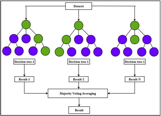
Figure 1. Random Forest algorithm.

This Random Forest flowchart of Figure 2 shows how to use the Random Forest algorithm for prediction problems in general. To ensure dependable model building, the procedure starts with data preparation, in which the dataset is gathered, arranged, and separated into training, testing, and validation subsets. In order to produce predictions, the model is subsequently tested on the remaining subsets after being trained on the training data. Lastly, assessment measures like MAPE, RMSE, and MAE are used to evaluate its accuracy and robustness, guaranteeing consistent performance across unknown data and real-world circumstances [14].

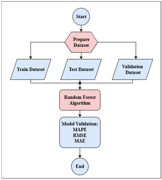
Figure 2. Flowchart of random forest.

Earlier RF outputs exceeded the physical limits due to incorrect inverse scaling during preprocessing. This issue was corrected by reapplying Min–Max normalization consistently across training and test datasets before retraining the model.

2.2.2. Long Short-Term Memory (LSTM)

A recurrent neural network type called LSTM was created to solve the vanishing gradient issue, which makes it useful for time series forecasting. Because wind power generation is heavily impacted by the weather, it is inherently a time-dependent process. LSTM can capture these temporal patterns [15].

The Figure 3 is the model of LSTM, and it relies on three main gates- forget, input, output- controlled by the sigmoid function, while the cell and input states are typically processed using the tanh function. LSTM’s structure allows it to learn complex relationships in nonlinear data [9].

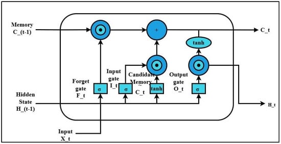
Figure 3. LSTM Structure.

The following collection of equations describes the LSTM:

Forget gate: The information from the prior cell state that is kept or destroyed is decided by the forget gate. Each unit is given a value between 0 and 1 using sigmoid activation, where 0 denotes total removal and 1 denotes complete retention [16].

$${\mathrm{f}}_{\mathrm{t}}=\mathrm{g}\left({\mathrm{w}}_{\mathrm{f}}\cdot \left[{\mathrm{h}}_{\mathrm{t}-1},{\mathrm{x}}_{\mathrm{t}}\right]+{\mathrm{b}}_{\mathrm{f}}\right)$$

(4)

Input gate: The input gate controls how fresh data are incorporated into the cell state. While a tanh layer creates a candidate vector of new values, a sigmoid activation determines which elements need to be changed. Incoming information may be selectively integrated into the cell state thanks to this technique.

$${\mathrm{i}}_{\mathrm{t}}=\mathrm{g}\left({\mathrm{w}}_{\mathrm{i}}\cdot \left[{\mathrm{h}}_{\mathrm{t}-1},{\mathrm{x}}_{\mathrm{t}}\right]+{\mathrm{b}}_{\mathrm{i}}\right)$$

(5)

State update:

$$\overline{{\mathrm{c}}_{\mathrm{t}}}=\tanh ({\mathrm{w}}_{\mathrm{c}}\cdot \left[{\mathrm{h}}_{\mathrm{t}-1},{\mathrm{x}}_{\mathrm{t}}\right]+{\mathrm{b}}_{\mathrm{c}})$$

(6)

$${\mathrm{C}}_{\mathrm{t}}={\mathrm{f}}_{\mathrm{t}}\cdot {\mathrm{C}}_{\mathrm{t}-1}+{\mathrm{i}}_{\mathrm{t}}\cdot \overline{{\mathrm{C}}_{\mathrm{t}}}$$

(7)

Output gate: The next hidden state, which is utilized as input for the next step and for predictions, is determined by the output gate. First, the components of the cell state that are conveyed are chosen using a sigmoid activation. The concealed state is then created by modulating the output of the sigmoid gate after the cell state has been changed using a tanh function.

$${\mathrm{o}}_{\mathrm{t}}=\mathrm{g}\left({\mathrm{w}}_0\cdot \left[{\mathrm{h}}_{\mathrm{t}-1},{\mathrm{x}}_{\mathrm{t}}\right]+{\mathrm{b}}_0\right)$$

(8)

$${\mathrm{h}}_{\mathrm{t}}={\mathrm{O}}_{\mathrm{t}}\cdot \tan \mathrm{h}\left({\mathrm{c}}_{\mathrm{t}}\right)$$

(9)

where ${\mathrm{w}}_{\mathrm{i}\mathrm{j}}$ represents the weight of neurons i to j, and b represents the bias.

The LSTM model was developed using a two-layer stacked architecture with 128 and 64 neurons, designed to capture both short- and medium-range temporal dependencies in the input data. A 56-step input window (approximately 4.7 h of historical measurements) was used to provide sufficient temporal context, and the model produced a 12-step-ahead forecast consistent with the 5 min sampling interval. The hidden layers used the tanh activation function, and a 20% dropout rate was applied to mitigate overfitting. The model was trained with a batch size of 32, which falls within the commonly used range of from 32 to 256 in time-series neural network applications, and was optimized over 50 epochs. Training employed the Adam optimizer with a learning rate of 0.001 and default momentum parameters (β₁ = 0.9, β₂ = 0.999). This configuration offered a practical balance between convergence, stability, and predictive accuracy for short-term renewable power forecasting.

The Figure 4 is the process of creating and assessing an LSTM model is shown in this flowchart. Data gathering comes first, then processing and standards. After that, the data are divided into test and training/validation sets. Training data are used to construct and train the LSTM model. The model is further optimized if it performs poorly. The procedure ends when the model is tested using the test data, and satisfactory performance is attained [17].

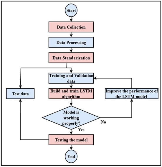
Figure 4. Flowchart of LSTM.

2.2.3. Artificial Neural Network (ANN)

The ability to recognize patterns and nonlinear correlations in complicated datasets is a feature of artificial neural networks, which are computer models modeled after the human brain. Modern energy systems can use them for time-series forecasting because of their capacity to capture complex relationships [10].

An input layer, one or more hidden layers, and an output layer of neurons make up a standard ANN. After applying nonlinear activation and computing a weighted sum of inputs, each neuron transmits the outcome. Accurate forecasts are made possible by optimizing weights via gradient descent and backpropagation to reduce prediction error [18].

In power forecasting applications, ANNs use features such as timestamps, weather variables, and historical power data to learn temporal and environmental influences on generation [19].

A basic ANN model for power forecasting can be described mathematically by the following equation:

$$\widehat{{\mathrm{y}}_{\mathrm{t}}}=\mathrm{f}(\mathrm{W}{\mathrm{x}}_{\mathrm{t}}+\mathrm{b})$$

(10)

where $\widehat{{\mathrm{y}}_{\mathrm{t}}}$ is the predicted output (e.g., power generation or consumption at time t);

• ${\mathrm{x}}_{\mathrm{t}}$ is the input vector at time t, which includes features like weather conditions or previous power values;
• W is the weight matrix associated with the connections between neurons;
• b is the bias vector;
• f is the activation function that introduces non-linearity into the model.

The Figure 5 shows the architecture and performance of ANNs and can vary depending on the number of hidden layers, the type of activation functions used (e.g., sigmoid, tanh, ReLU), and the learning rate of the training process. To enhance forecasting accuracy, techniques such as dropout, early stopping, and batch normalization may be applied during training [20].

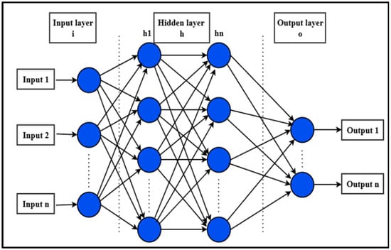
Figure 5. ANN structure.

ANNs continue to be a reliable and adaptable forecasting tool in the energy sector, offering robust performance even when dealing with noisy, incomplete, or highly variable data input. Their widespread adoption in smart grid and renewable energy forecasting applications underscores their importance in supporting efficient energy management and planning [12].

The ANN model was designed with a feed-forward architecture comprising three hidden layers with 256, 128, and 64 neurons, respectively. Each hidden layer employed the ReLU activation function to support effective learning of nonlinear relationships, and 30% dropout was applied across all hidden layers to reduce overfitting. Batch normalization was performed after every hidden layer to stabilize training and improve convergence. The network produced a 12-dimensional output vector, corresponding to a 1 h-ahead forecast at a 5 min resolution. Model training was conducted with a batch size of 32 and extended over 100 epochs, allowing the network adequate iterations to refine its internal weights. Optimization was performed using the Adam optimizer, with a learning rate tuned within the range from 0.001 to 0.01, depending on validation performance. Model development followed a progressive strategy in which a simpler structure was trained first and then gradually deepened, ensuring an appropriate balance between model complexity and generalization capability.

Figure 6 shows the flowchart of the Artificial Neural Network process, starting with loading and preprocessing the dataset, including tasks like cleaning and normalization. After that, an ANN model is developed based on a selected method suitable for the problem. After that, the model’s performance is assessed by testing and training. The model is put into use if the resting accuracy is acceptable. If not, the process checks whether to improve the model architecture or enhance the dataset. Depending on this decision, adjustments are made, and the model is retrained. This cycle continues until the desired accuracy is achieved, at which point the model is finalized and deployed [21].

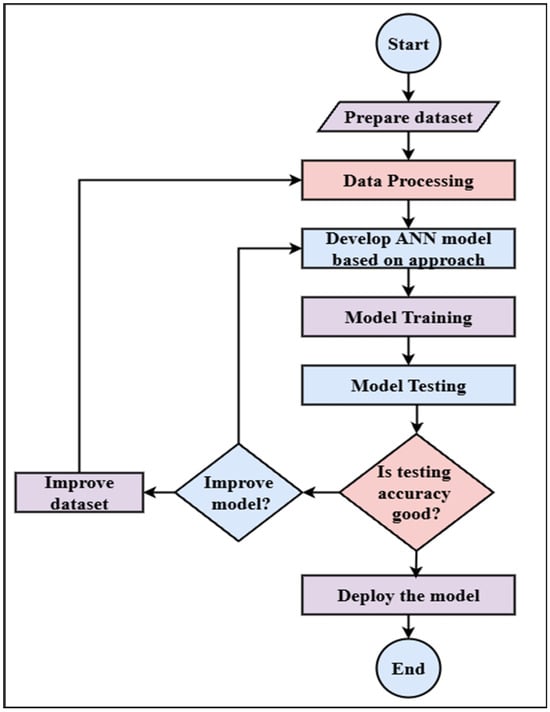
Figure 6. Flowchart of ANN.

3. Results

This presents the comparative performance of three computational models, such as ANN, LSTM, and Random Forest, which were developed for short-term forecasting of solar and wind power generation in isolated microgrids. The models were tested by incorporating meteorological parameters such as solar irradiance and wind speed. Model performance was evaluated using Mean Absolute Error, Root Mean Square Error, and Mean Absolute Percentage Error. The results indicate that all three approaches effectively capture complex temporal variations in renewable power output, with noticeable performance enhancements when meteorological inputs are included in the prediction framework.

This will describe the accuracy of the results through the following:

1.

Root Mean Square Error (RMSE): A popular statistic for assessing forecast accuracy is RMSE. It calculates the difference between the actual observed values and the expected values [22].

$$\mathrm{RMSE}=\sqrt{{\displaystyle \frac{1}{n}}{\sum }_{i=1}^n({y_i-\widehat{y_i})}^2}$$

(11)

where $y_i$ are the predicted values, and $\widehat{y_i}$ is the actual values. n is the length of the forecasted values.

2.

Mean Absolute Percentage Error (MAPE): A statistical metric for assessing a forecasting model’s accuracy is the MAPE. It displays predicted mistakes as a promotion of the values that were observed [23].

$$\mathrm{MAPE}={\displaystyle \frac{1}{n}}{\sum }_{i=1}^n\left|{\displaystyle \frac{y_i-\widehat{y_i}}{y_i}}\right|\times 100$$

(12)

where $y_i$ are the predicted values and $\widehat{y_i}$ is the actual values. n is the length of the forecasted values.

3.

Mean Absolute Error: The MAE is a widely used tool to assess how accurate forecasts or predictions are. It shows the typical absolute difference between the actual and forecasted values [24].

$$\mathrm{MAE}={\displaystyle \frac{1}{n}}{\sum }_{i=1}^n\left|y_i-\widehat{y_i}\right|$$

(13)

where $y_i$ are the predicted values and $\widehat{y_i}$ is the actual values. n is the length of the forecasted values.

Figure 7 compares the actual measured power output (blue line) with values predicted by the Random Forest model (orange line). While the actual data exhibit a realistic and stable generation pattern, the RF model significantly overpredicts output, particularly between indices 120 and 240, reaching peaks above 5000 units, whereas actual values remain below 1000. This discrepancy suggests overfitting or insufficient feature representation in the RF model, highlighting the need for further optimization to enhance forecasting accuracy in power generation applications.

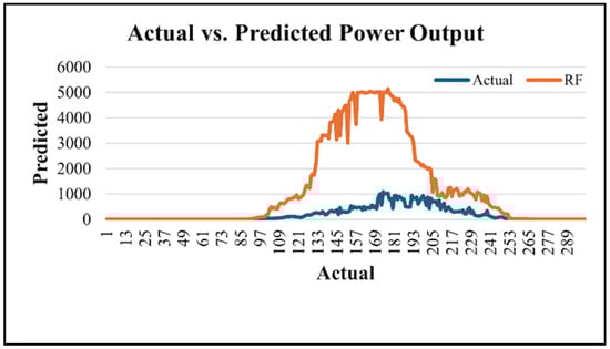
Figure 7. Random Forest algorithm results in kW.

Figure 8 illustrates the comparison of actual Random Forest (RF) and predicted power output over three years. The RF model follows the general trend but overestimates values during peak generation, indicating the need for improved accuracy in capturing fluctuation.

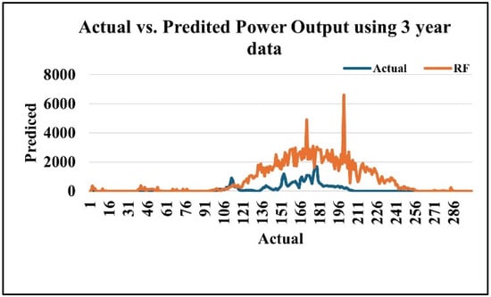
Figure 8. Random Forest algorithm results using the three-year dataset in kW.

Figure 9 shows the comparison between the actual Random Forest (RF) predicted power output using one year of data. The RF model captures the overall seasonal pattern but consistently overestimates the magnitude of generation, indicating the need for further refinement.

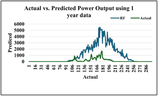
Figure 9. Random Forest algorithm results using the one-year dataset in kW.

Figure 10 compares the Random Forest (RF) predictions with the actual power output across six months. While the model follows the general trend of the data, it tends to overestimate during high-output periods, leading to noticeable deviations at peak values.

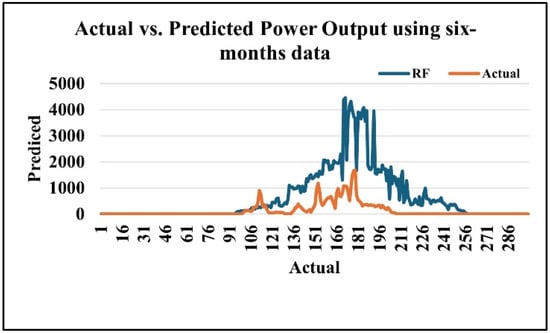
Figure 10. Random Forest algorithm results using the six-month dataset in kW.

As per the comparison of MAE, the six-month dataset gives the highest accuracy. However, the three-year dataset provides the most balanced and consistent prediction accuracy, confirming that an adequate span of historical data improves model reliability and forecasting stability in renewable energy-based microgrids (Table 3).

Table 3. Comparison of different datasets’ accuracy with RF.

Dataset	MAE (kW)
FOUR-YEAR	600.5481
THREE-YEAR	377.00069
ONE-YEAR	528.0792
SIX-MONTHS	304.5129

Figure 11 compares actual and Random Forest-predicted power output over a daily cycle. The model closely follows the observed trend, capturing the morning increase, midday peak, and evening decline, with only minor deviations.

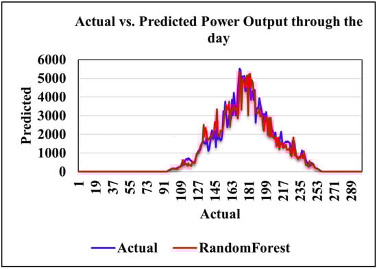
Figure 11. Random Forest through the day in kW.

Figure 12 compares actual and forecasted power output from the LSTM model over one week. Using 56 input sequences and 50 training epochs, the model achieved a Mean Absolute Error of 97.52 kW, demonstrating strong predictive accuracy.

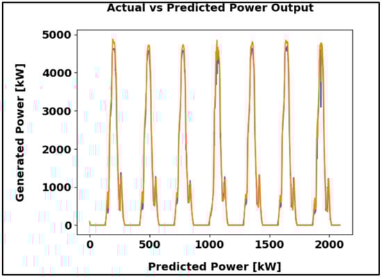
Figure 12. LSTM algorithm results in kW.

The observed overestimation demonstrates that the Random Forest model is more sensitive to scaling inconsistencies than the ANN and LSTM models, which produced stable outputs within the physical generation range.

Figure 13 compares actual and predicted power output over three years, showing strong agreement between both trends. With a Mean Absolute Error (MAE) of 101.73 kW, the model demonstrates high accuracy and reliable performance.

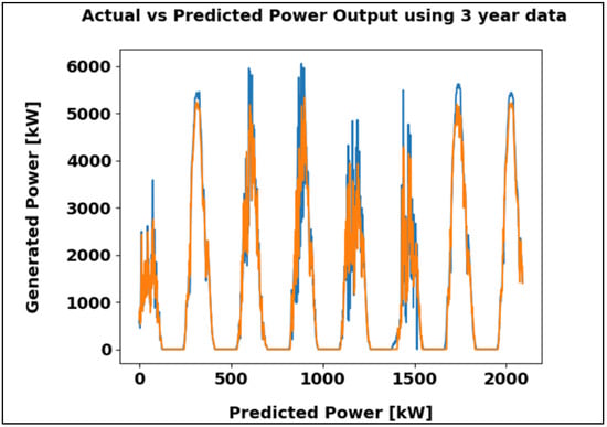
Figure 13. LSTM algorithm result using the three-year dataset in kW.

Figure 14 illustrates the comparison between actual and predicted power output for one year of data, revealing a strong correlation between the two. The MAE of 61.92 kW reflects precise estimation and consistent performance of the model.

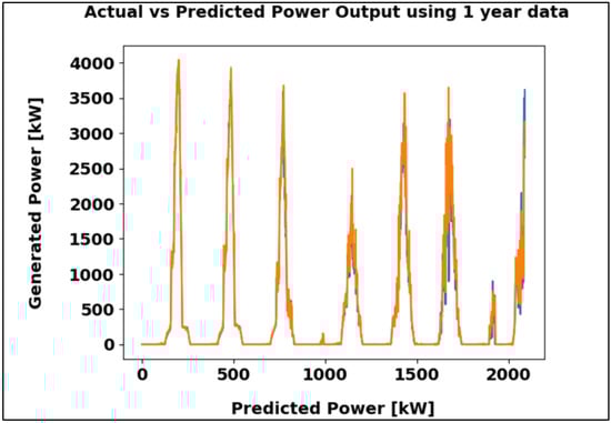
Figure 14. LSTM algorithm result using the one-year dataset in kW.

Figure 15 presents a comparison between actual and predicted power output over six months, showing a close match between both curves. The MAE of 48.98 kW indicates precise prediction and strong model reliability.

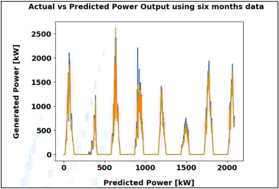
Figure 15. LSTM algorithm result using the six-month dataset in kW.

Among these, the six-month dataset shows the lowest MAE of 48.98 kW, indicating the most accurate and consistent prediction results. In contrast, longer datasets display slightly higher errors, likely due to increased variations over extended periods (Table 4).

Table 4. Comparison of different datasets’ accuracy with LSTM.

Dataset	MAE (kW)
FOUR-YEAR	97.52
THREE-YEAR	101.73
ONE-YEAR	61.92
SIX-MONTHS	48.98

Figure 16 shows the comparison between actual and predicted power outputs over 7-day intervals across 2000-time steps. The blue line denotes observed data, while the orange line represents model predictions. The recurring pattern indicates periodic demand, and the close alignment confirms strong predictive accuracy.

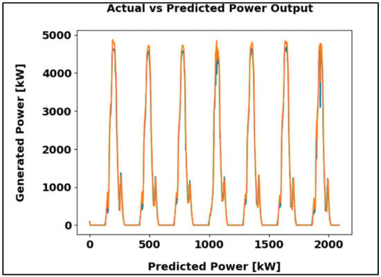
Figure 16. ANN algorithm results in kW.

Figure 17 compares actual and predicted power output over a three-year period. The strong overlap between the observed and estimated values indicates that the model captures long-term generation trends effectively. The performance is supported by a Mean Absolute Error of 117.44 kW, demonstrating its suitability for extended forecasting.

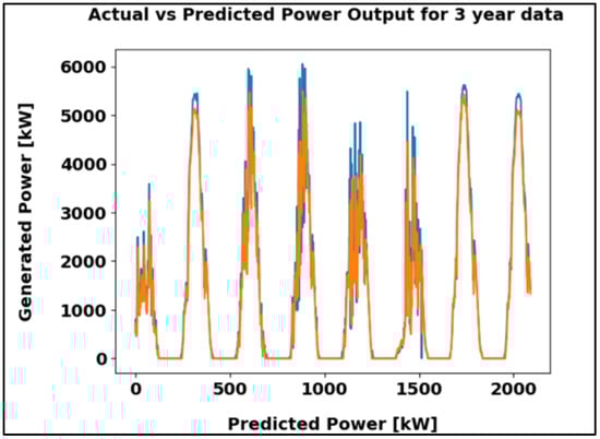
Figure 17. ANN algorithm result using the three-year dataset in kW.

Figure 18 compares actual and predicted power output over one year in 7-day intervals. The close alignment of the two curves indicates effective tracking of generation patterns, further supported by a Mean Absolute Error 0f 64.72 kW, which is low relative to the maximum output of approximately 4000 kW.

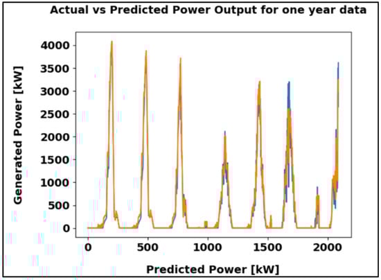
Figure 18. ANN algorithm results using the one-year dataset in kW.

Figure 19 compares actual and predicted power output over six months, with the blue line showing actual values and the orange line representing predictions. The close alignment of both curves highlights the model’s accuracy, further supported by a Mean Absolute Error of 65.92 kW, confirming its effectiveness for reliable energy forecasting.

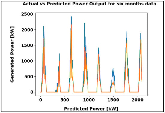
Figure 19. ANN algorithm result using the six-month dataset kW.

As per the comparison of MAE, the one-year dataset gives the highest accuracy. However, the three-year dataset provides the most balanced and consistent prediction accuracy, confirming that an adequate span of historical data improves model reliability and forecasting stability in renewable energy-based microgrids (Table 5).

Table 5. Comparison of different dataset’s accuracy with ANN.

Dataset	MAE (kW)
FOUR-YEAR	256.24
THREE-YEAR	117.44
ONE-YEAR	64.72
SIX-MONTHS	65.92

To maintain consistency throughout the analysis, all error values (MAE, RMSE, and MAPE) were re-verified and aligned across datasets and models. The ANN demonstrated the lowest MAE in each comparable dataset, achieving 64.72 kW for the one-year period. LSTM produced an MAE of 97.52 kW, while Random Forest recorded substantially higher errors, including 304.51 kW for the six-month dataset. These corrected values ensure uniformity in all tables and model comparisons (Table 6).

Table 6. Accuracy comparison with different models.

Methods	MAE (kW)
RANDOM FOREST	304.51
LSTM	97.52
ANN	64.72

The error metrics were cross-checked for consistency, and ANN achieved the lowest MAE (64.72 kW), followed by LSTM (97.52 kW), while Random Forest showed the highest deviations. Considering that the microgrid’s average renewable output is about 1.4 kW, the ANN error corresponds to roughly 4–5% of typical generation. This level of accuracy is generally sufficient for short-term scheduling and has minimal impact on reserve allocation or generator dispatch. In contrast, LSTM errors represent about 7% of the average output, and Random Forest errors exceed 20%, which would require higher reserve margins and more frequent cycling of backup units.

Across all datasets, ANN consistently provided the most stable and accurate forecasts, while LSTM performed moderately well during transitional periods, and Random Forest tended to overestimate during high-output intervals. These differences reflect the inherent characteristics of the models. From an operational perspective, the lower ANN error supports more efficient battery management and reduced reliance on diesel generators, making it the most practical option for short-term microgrid forecasting.

4. Conclusions

This study presented a comparative assessment of three machine-learning models—Random Forest, Artificial Neural Network (ANN), and Long Short-Term Memory (LSTM)—for short-term forecasting of solar and wind power generation in a microgrid setting. All models were developed using a consistent preprocessing and feature-engineering framework to ensure a fair evaluation of their predictive performance. Among the three techniques, the ANN demonstrated the strongest forecasting capability, achieving the lowest MAE of 64.72 kW on the one-year dataset and effectively capturing nonlinear fluctuations in renewable generation. The LSTM model performed competitively, particularly during transitional periods when sequential patterns were more prominent, while the Random Forest model showed the highest error levels and a clear tendency to overestimate peak generation, largely due to its sensitivity to scaling and rapid meteorological variations. When interpreted relative to the microgrid’s typical generation level of approximately 1.4 kW, the ANN’s error corresponds to only about 4–5%, which is generally acceptable for short-term scheduling and reserve planning.

In contrast, the higher errors associated with LSTM and RF would require more conservative operating margins and could lead to less efficient generator cycling. Accordingly, the contribution of this work lies in providing a detailed, evidence-based comparison of commonly used forecasting techniques rather than proposing a hybrid or integrated energy-management framework. While improved forecast accuracy can support more stable microgrid operation, this study focuses solely on predictive performance; future research will incorporate these models into dispatch simulations to quantify their influence on reserve allocation, diesel-generator scheduling, and battery cycling. Overall, the findings offer practical insight into model selection for renewable energy forecasting and support the continued development of data-driven tools for microgrid applications.

References

- Sharker, M.N.; Alam, M.A.; Tamal, M.B.A.; Sazid, M.I. A High Performing Approach to Short-Term PV Power Forecasting using Machine Learning Algorithms. In Proceedings of the 2023 10th IEEE International Conference on Power Systems (ICPS), Cox’s Bazar, Bangladesh, 13–15 December 2023; pp. 1–6. [Google Scholar]
- Ahmed, Z.; Mohsin, J.; Khan, A. A Novel Multi-Task Learning-Based Approach to Multi-Energy System Load Forecasting. IEEE Open Access J. Power Energy 2025, 12, 209–219. [Google Scholar] [CrossRef]
- Khan, I.U.; Jamil, M. Hybrid Long Short-Term Memory (LSTM) and Exponentially Weighted Moving Average (EWMA) Model for Accurate and Scalable Electricity Price Forecasting. In Proceedings of the 2025 IEEE 13th International Conference on Smart Energy Grid Engineering, Oshawa, ON, Canada, 20 August 2025. [Google Scholar]
- Patel, V.R.; Patel, M.S.; Patel, M.U.; Patel, T.C.; Patel, M.R. Solar Power Generation Forecasting Using Adaptive Boost and Random Forest. Int. J. Darshan Inst. Eng. Res. Emerg. Technol. 2022, 11, 2. [Google Scholar] [CrossRef]
- Jin, X.; Han, R.; Ma, Y. PV Power Forecasting Based on VMD-RIME-LSTM. In Proceedings of the 2024 IEEE China International Youth Conference on Electrical Engineering (CIYCEE), Wuhan, China, 6–8 November 2024; pp. 1–5. [Google Scholar]
- Yamini, S.; Sistla, H.R.; Suman, T.; Sravani, D.; Rajeswaran, N.; Deenababu, M. Enhancing Smart Grid Management: Load Forecasting, Power Grid Stability Assessment, and Fault Detection using Artificial Neural Networks. In Proceedings of the 2024 10th International Conference on Advanced Computing and Communication Systems (ICACCS), Coimbatore, India, 14–15 March 2024; pp. 1098–1102. [Google Scholar]
- Azman, M.; Jantan, H.; Bahrin, U.M.; Kadir, E. Solar Power Production Forecasting Model Using Random Forest Algorithm. In Intelligent Systems Design and Applications; Springer: Cham, Switzerland, 2024; pp. 133–144. [Google Scholar]
- Jamii, J.; Trabelsi, M.; Mansouri, M.; Mimouni, M.F. An Effective Random Forest based Long-Term Wind Power Forecasting Technique. In Proceedings of the 2023 20th International Multi-Conference on Systems, Signals & Devices (SSD), Mahdia, Tunisia, 20–23 February 2023; pp. 586–590. [Google Scholar]
- Raji, K.; Hamamalini, S. Long short-term memory-based forecasting of uncertain parameters in an islanded hybrid microgrid and its energy management using improved grey wolf optimization algorithm. IET Renew. Power Gener. 2024, 18, 3640–3658. [Google Scholar]
- Gaboitaolelwe, J.; Zungeru, M.A.; Yahya, A.; Lebekwe, C.; Naga, V.D.; Salau, A. Machine Learning Based Solar Photovoltaic Power Forecasting: A Review and Comparison. IEEE Access 2023, 11, 40820–40845. [Google Scholar] [CrossRef]
- Huang, Z.; Jiang, J.; Ma, W.; Liu, K.; Zou, L. Forecast of Power Grid Material Demand Based on Random Forest. In Proceedings of the 2022 International Conference on Artificial Intelligence in Everything (AIE), Lefkosa, Cyprus, 2–4 August 2022; pp. 227–231. [Google Scholar]
- Ahmed, Z.; Jamil, M.; Khan, A. Short-Term Campus Load Forecasting Using CNN-Based Encoder–Decoder Network with Attention. Energies 2024, 17, 4457. [Google Scholar] [CrossRef]
- Dudek, G. A Comprehensive Study of Random Forest for Short-Term Load Forecasting. Energies 2022, 15, 7547. [Google Scholar] [CrossRef]
- Villegas, C.G.; Rodriguez, J.; Carrera, L.A.I.; Ramírez, J.M.O.; Martínez-Gutiérrez, H.; Marrínez, E.N.R. Optimized Random Forest for Solar Radiation Prediction Using Sunshine Hours. Micromachines 2022, 13, 9. [Google Scholar] [CrossRef] [PubMed]
- Wu, J.; Lin, R.; Pan, M.; Wang, B.; Wang, O.; Zhao, Q.; Liu, H. Load Forecasting Method Considering Weather Factors based on LSTM and XGBoost. In Proceedings of the 2024 IEEE 24th International Conference on Communication Technology (ICCT), Chengdu, China, 18–20 October 2024; pp. 2021–2026. [Google Scholar]
- Arya, T.; Sharma, A. Solar Power Forecasting Using Machine Learning and Deep Learning. Int. J. Creat. Res. Thoughts 2024, 12, c952–c959. [Google Scholar]
- Olcay, K.; Tunca, S.G.; Özgür, M. Forecasting and Performance Analysis of Energy Production in Solar Power Plants Using Long Short-Term Memory (LSTM) and Random Forest Models. IEEE Access 2024, 12, 103299–103312. [Google Scholar] [CrossRef]
- Ananthi, K.; Sownthariya, M.; Ranjana, E.; Moulieshwaran, K.; Babu, B.S. An Insight of Deep Neural Networks Based on Demand Forecasting in Using: Ann Algorithm. In Proceedings of the 2024 10th International Conference on Advanced Computing and Communication Systems (ICACCS), Coimbatore, India, 14–15 March 2024; pp. 2469–2472. [Google Scholar]
- Jamil, M.; Khan, M.N.; Rind, S.J.; Awais, Q.; Uzair, M. Neural Network Predictive Control of Vibrations in Tall Structure: An Experimental Controlled Vision. J. Comput. Electr. Eng. 2021, 89, 106940. [Google Scholar] [CrossRef]
- Blinov, I.; Miroshnyk, V.; Shymaniuk, P. Short-term Nodal Electrical Load Forecasting with Artificial Neural Networks. In Proceedings of the 2022 IEEE 8th International Conference on Energy Smart Systems (ESS), Kyiv, Ukraine, 12–14 October 2022; pp. 13–16. [Google Scholar]
- Sharma, A.; Indliya, J.N.; Swami, R.K.; Gupta, S. Generation Forecasting of Solar PV in Distribution Network using ANN. In Proceedings of the 2023 2nd International Conference on Automation, Computing and Renewable Systems (ICACRS), Pudukkottai, India, 11–13 December 2023; pp. 156–161. [Google Scholar]
- Nezhadkhatami, H.; Hajizadeh, A.; Soltani, M.; Guilbert, D. Variant Parameters Identification of the PEMEL Circuit Model by RMSE-Based Self-Tuning Method. In Proceedings of the 2023 IEEE 32nd International Symposium on Industrial Electronics (ISIE), Helsinki, Finland, 19–21 June 2023; pp. 1–6. [Google Scholar]
- Khowarizmi, A.; Efendi, S.; Nasution, M.K.; Herman, M. The Role of Detection Rate in MAPE to Improve Measurement Accuracy for Predicting FinTech Data in Various Regressions. In Proceedings of the 2023 International Conference on Computer Science, Information Technology and Engineering (ICCoSITE), Jakarta, Indonesia, 16 February 2023; pp. 874–879. [Google Scholar]
- Cheng, Y.; Zhang, L. MAE-Based Radio Map Construction for Wi-Fi Fingerprint Indoor Localization. IEEE Commun. Lett. 2025, 29, 2008–2012. [Google Scholar] [CrossRef]
Disclaimer/Publisher’s Note: The statements, opinions and data contained in all publications are solely those of the individual author(s) and contributor(s) and not of MDPI and/or the editor(s). MDPI and/or the editor(s) disclaim responsibility for any injury to people or property resulting from any ideas, methods, instructions or products referred to in the content. |
© 2026 by the authors. Licensee MDPI, Basel, Switzerland. This article is an open access article distributed under the terms and conditions of the Creative Commons Attribution (CC BY) license.