Data-Driven Estimation of Transmission Loss Coefficients via Linear and Quadratic Programming Under Linear Constraints

Abstract

This paper presents a robust data-driven methodology for estimating transmission loss coefficients (B-coefficients) in power systems using linear and quadratic programming (LP and QP), both of which belong to the family of convex optimization models. The first model employs a linear objective function with linear constraints, ensuring computational efficiency for simpler scenarios. The second model utilizes a quadratic objective function, also under linear constraints, to better capture more complex nonlinear relationships. By framing the estimation problem as a parameter identification task, both methodologies minimize the cost functions that quantify the mismatch between measured and modeled power losses. By considering a broad range of operational scenarios, our approach effectively captures the stochastic behavior inherent in power system operations. The effectiveness of both the LP and QP models is validated in terms of their ability to accurately extract physically meaningful B-coefficients from diverse simulation datasets. This study underscores the potential of integrating linear and quadratic programming as powerful and scalable tools for data-driven parameter estimation in modern power systems, especially in environments characterized by uncertainty or incomplete information.

1. Introduction

Optimizing generation schedules and enhancing the operating efficiency of electrical power systems is an inherently complex task that requires detailed understanding and accurate modeling of the power flows and associated losses within a network [1]. Power transmission losses exhibit a nonlinear behavior influenced by numerous factors, including load demands, generation profiles, network configuration, and electrical parameters [2]. To accurately quantify these energy dissipations, B-coefficients are employed as essential parameters within power flow models, representing the quadratic components of the loss equations [3]. The precise estimation of these coefficients is vital for ensuring that dispatch solutions are reliable, cost-efficient, and consistent with operational constraints, ultimately leading to improved system performance and sustainability [4].

The significance of accurately estimating B-coefficients extends beyond immediate operational decisions, as it also impacts long-term planning processes. Reliable coefficients allow system operators to better predict transmission losses, which in turn helps to reduce their operating expenses and environmental footprint through optimized generation strategies [5]. Additionally, a detailed knowledge of B-coefficients aids the integration of renewable energy sources, given their inherent variability and unpredictability—factors that directly affect losses in transmission systems [6]. Consequently, the accuracy of these parameters influences the grid’s stability, resilience, and capacity to evolve without sacrificing efficiency or dependability [7,8].

Historically, methods for estimating B-coefficients have utilized a broad range of approaches, including analytical procedures, measurement-based techniques, and convex optimization models [5]. For instance, analytical methods like Kron reduction provide rapid estimates but often oversimplify the complexities inherent in real transmission networks, potentially leading to inaccuracies [3,9]. Conversely, measurement-based approaches—relying on data from supervisory control and data acquisition (SCADA) systems or phasor measurement units (PMUs)—require comprehensive and high-quality datasets, which can be challenging to collect and process reliably. While convex optimization strategies are robust and mathematically sound, they typically impose linearity or convexity assumptions that may not adequately capture the nonlinear and uncertain behaviors of actual power systems. These limitations underscore the necessity for more advanced, flexible, and data-driven estimation techniques [10]. Such approaches should have the ability to model the dynamic and unpredictable nature of modern electrical grids, ultimately improving the accuracy and reliability of B-coefficient estimations.

The formulation of linear programming (LP) and quadratic programming (QP) models with linear constraints plays a crucial role in addressing the complex challenges associated with parameter estimation in transmission networks. This study introduces an innovative data-driven methodology for estimating transmission loss coefficients—commonly referred to as B-coefficients—that leverages LP and QP techniques.

Traditional convex optimization methods often face significant limitations due to their dependence on gradient information and convexity constraints. These factors can restrict applicability in real-world scenarios characterized by complex loss behaviors [11]. In response, our proposed approach reconceptualizes the estimation process as a parameter identification problem, aiming to minimize a well-defined cost function that quantifies the differences between simulated measurement data. These data realistically reflect the variations seen in power generation and load profiles, enhancing the accuracy of modeled transmission losses.

A key strength of this methodology is its ability to accommodate a wide range of operating conditions, effectively addressing the stochastic and nonlinear nature of power systems operation [12]. By exploring various scenarios during the optimization process, our model improves the robustness and physical relevance of the estimated coefficients, ensuring they accurately capture the true dynamics of the system [11]. This flexibility is vital for enhancing modeling accuracy, which is essential for operational planning, reliability assessments, and the successful integration of renewable energy sources.

Ultimately, this approach represents a significant advancement in power grid management. By demonstrating their importance in modern electrical engineering, this work emphasizes the potential of LP and QP models to aid in designing more efficient and resilient power systems, thus contributing to the overall sustainability of energy networks.

The estimation of B-coefficients has been a topic of considerable interest within power systems research, leading to the development of various analytical, measurement-based, and optimization-driven techniques. Initial studies, such as [13], employed Kron reduction methods to directly compute these coefficients from network parameters, offering computational efficiency at the expense of accuracy due to the simplifications and assumptions inherent in the approach. As measurement technology advanced, researchers began to utilize real-time data to enhance estimation accuracy. Methods utilizing SCADA systems laid the groundwork for measurement-based estimation, which was further refined with the advent of PMUs. These tools enable high-resolution, synchronized data collection, facilitating the real-time tracking of power losses and dynamic parameter estimation [14,15].

Furthermore, the authors of [16] presented a novel method for calculating B-coefficients that addresses the limitations of traditional approaches. This method is characterized by its speed and ability to handle line outages, utilizing network sensitivity factors derived from DC load flow solutions. The authors formulated line outage distribution factors (ODFs) based on changes in network power generation, eliminating the need for complex Kron tensor analysis and data normalization. This method demonstrated a competitive performance in terms of solution speed and accuracy against existing methods, making it well-suited for online dispatch applications.

The work by [17] explored various optimization techniques for solving the optimal power flow (OPF) problem in power systems, emphasizing the traditional use of B-coefficient formulas for calculating power losses. The authors discussed the common assumption of a constant ratio between reactive and active power generation, revealing its limited validity. Furthermore, they introduced an alternative assumption that derives B-coefficients based on constant generation reactive power, which yielded superior results compared to the conventional method when tested on two power systems, including the IEEE-26 bus system.

In [18], empirical approaches for calculating the power loss factor in electrical systems were explored, utilizing methods such as machine learning and statistical analysis. This study combined actual data with computed loss factors, demonstrating that exponential curve fitting effectively correlates load and loss factors. Tested on two distribution substations in Karbala, Iraq, the approach yielded an average yearly loss factor of 0.6114. This was achieved using the ETAP software, showcasing the method’s robustness compared to other solutions.

The authors of [19] presented an evaluation of A loss coefficients for analyzing transmission losses in the context of the dynamic economic dispatch (DED) problem. They compared losses computed with nominal A- and B-coefficients against the results of the standard Newton–Raphson method (NRM). Using the density-based clustering method (DBSCAN), they identified optimal regions for these coefficients. This work introduced a novel approach to improve the accuracy of network loss calculations by updating loss coefficients based on changes in per-unit load values. The proposed algorithm was validated on various IEEE feeders, including the 6-, 14-, 30-, and 118-bus systems, using SCILAB 5.4.

In recent years, data-driven and hybrid methodologies have gained significant traction in the estimation of B-coefficients. Techniques such as least squares regression [3], genetic algorithms (GA) [20], and particle swarm optimization (PSO) have been employed to enhance robustness in the face of measurement noise and system uncertainties. These approaches often incorporate models that account for renewable generation variability, load fluctuations, and changes in network topology, offering greater adaptability to real-world operating conditions. Additionally, machine learning methods and nonlinear regression models have been explored to improve estimation accuracy under highly uncertain environments. Despite these advances, many existing methods still exhibit difficulties in fully capturing the inherently nonlinear and stochastic nature of power system losses, especially when operating under dynamic scenarios with incomplete or noisy data.

More recently, the development of convex measurement-based approaches leveraging semidefinite programming (SDP) has shown promising results. Notably, the authors of [5] proposed an SDP-based framework that utilizes power flow solutions derived from measurement data while explicitly incorporating stochastic variations in demand and generation. Their methodology involves repeatedly solving the power flow problem using the NRM while modeling fluctuations with Gaussian or uniform distributions, allowing for a robust estimation of transmission loss coefficients. Across multiple test networks, their approach achieved low estimation errors—around 3.4% on average—demonstrating its high accuracy and reliability. Extensive validation through numerical simulations on standard test feeders further underscored the effectiveness of measurement-driven convex optimization in accurately determining B-coefficients, making it a compelling strategy for modern power system analysis.

Building upon these developments, this research aims to leverage the capabilities of LP and QP models to address limitations related to nonlinearity and uncertainty in transmission networks. Unlike traditional methods, our approach extensively utilizes simulated measurement data that encompass a broad range of operational scenarios, including system topologies, outages, and load variations. This strategy not only enhances the adaptability of the estimation process but also ensures robustness against system uncertainties and measurement noise. Since it directly integrates diverse data scenarios into the optimization framework, our method is well-suited for real-time applications and dynamic system monitoring, providing more accurate and physically meaningful B-coefficient estimates, which are fundamental for ensuring a reliable power system operation as well as effective planning.

In this vein, the key contributions of this work are presented below.

• It introduces a novel data-driven estimation method for transmission loss B-coefficients based on two convex optimization models, i.e., LP and QP, within a parameter identification framework.
• It demonstrates that our convex-based approach effectively captures the nonlinear and stochastic nature of power system losses, making it suitable for complex estimation landscapes.
• It ensures the physical meaningfulness of the estimated B-coefficients by enforcing the positive semidefiniteness of the parameter matrix.

Within the scope of this study, measurement data are obtained from PMUs or generated via recursive power flow simulations, capturing the variability in power generation and demand. Our methodology employed the full NRM to accurately solve power flows within the network, which allowed considering the real part of the admittance matrix and effectively capture the transmission losses. This approach avoids the inaccuracies associated with ignoring critical components typically found in linear power-flow assumptions, particularly under dynamic operating conditions with fluctuating loads and generation profiles. Additionally, stochastic load variations were incorporated to further reflect the dynamics of the power system. The flexibility of our methodology supports the recalibration of the B-coefficients in response to system changes, enabling real-time adaptation in modern, uncertain power systems and providing a robust foundation for accurate estimation, thereby enhancing the reliability and physical relevance of our results.

The remainder of this research is organized as follows. Section 2 presents the theoretical framework for the B-coefficient estimation problem in power systems, utilizing a minimization approach with an equivalent quadratic model for power losses. Section 3 outlines the proposed solution methodology, which is divided into three stages. The first stage reformulates the optimization problem as an LP model, while the second stage addresses it as a QP problem. The third stage introduces a data-driven approach that employs recursive power flow solutions to account for varying operating conditions in generation sources and demand nodes, concluding with a summary of our proposal. Section 4 details the numerical validations conducted on various IEEE test feeders, including a comparative analysis of the proposed model against the iterative approach reported by the authors of [15]. Finally, Section 5 summarizes the main conclusions drawn from this work and presents potential avenues for future research.

2. General Problem Formulation

The transmission loss estimation problem can be framed as a general parameter identification task aimed at determining the unknown coefficients that best align with the observed data [5]. In this vein, let $\mathbf{M}$ represent the set of measurements (or power flow solutions for different operating conditions), each corresponding to a specific system state characterized by known power generation and demand values as well as measured power losses [15]. The primary objective is to minimize the discrepancy between the observed losses and those predicted by a mathematical model governed by the unknown parameters—namely, the coefficients $B_{20}$, $B_{10}$, and $B_{00}$.

The modeling process begins with the definition of an objective function that quantifies the error between the measured and modeled power losses. Formally, this can be expressed as the minimization of the sum of absolute deviations [3]:

$$\underset{B_{20},B_{10},B_{00}}{min}E=\sum _{m\in \mathbf{M}}|{\overline{P}}_{L_m}-P_{L_m}|,$$

(1)

where $P_{L_m}$ denotes the modeled power losses at measurement m, which depend on the unknown coefficients and the known power generation $P_{G_m}$ [13]:

$$P_{L_m}=P_{G_m}^{\top }{B}_{20}{P}_{G_m}+B_{10}^{\top }{P}_{G_m}+B_{00}.$$

(2)

This formulation is a flexible, general approach that does not impose specific structural constraints—such as positive semidefiniteness—on $B_{20}$. Instead, it incorporates basic physical and structural constraints to ensure meaningful solutions, e.g., assuming $B_{20}$ to be symmetric and diagonal positive based on empirical considerations [5]:

$$\begin{array}{cc}\hfill B_{20}& =B_{20}^{\top },\hfill \end{array}$$

(3)

$$\begin{array}{cc}\hfill \mathrm{diag}\left(B_{20}\right)& >0.\hfill \end{array}$$

(4)

Additionally, the constant term $B_{00}$ is constrained within a user-defined range:

$$\alpha \le B_{00}\le \beta ,$$

(5)

where $\alpha$ and $\beta$ are bounds based on physical, empirical, or theoretical considerations—often with $\alpha =0$.

The entire set of constraints is designed to reflect physical and structural properties relevant to power systems. Therefore, the resulting optimization problem aims to identify the coefficients that minimize the total error across measurements while satisfying the specified structural constraints:

$$\begin{array}{cc}\hfill \mathrm{Minimize}:& E=\sum _{m\in \mathbf{M}}|{\overline{P}}_{L_m}-P_{L_m}|,\hfill \\ \hfill \mathrm{Subject}\mathrm{to}:\end{array}$$

(6)

$$\begin{array}{cc}\hfill & P_{L_m}=P_{G_m}^{\top }{B}_{20}{P}_{G_m}+B_{10}^{\top }{P}_{G_m}+B_{00},\forall m\in \mathbf{M},\hfill \end{array}$$

(7)

$$\begin{array}{cc}\hfill & B_{10}^{\top }{P}_{G_m}\ge 0,\forall m\in \mathbf{M},\hfill \end{array}$$

(8)

$$\begin{array}{cc}\hfill & B_{20}=B_{20}^{\top },\hfill \end{array}$$

(9)

$$\begin{array}{cc}\hfill & \mathrm{diag}\left(B_{20}\right)>0,\hfill \end{array}$$

(10)

$$\begin{array}{cc}\hfill & \alpha \le B_{00}\le \beta ,\hfill \end{array}$$

(11)

This approach constitutes a broad, flexible framework capable of capturing nonlinear relationships between generation, demand, and system losses. It can be efficiently solved using optimization algorithms that do not require the structural properties imposed by SDP, thus providing a versatile and computationally tractable method for estimating transmission loss coefficients across diverse operational scenarios.

3. Proposed Reformulation and Solution Methodology

3.1. Linear Programming Modeling

In this research, the general formulation presented in Section 2, originally proposed by the authors of [5], was transformed into an LP model by means of a single modification. This adjustment does not compromise the effectiveness of the transmission loss coefficient estimation methodology.

3.1.1. Objective Function Transformation

To transform the nonlinear objective $minz=\left|f\right(x\left)\right|$ into a linear form, an auxiliary variable $t\ge 0$ that represents the magnitude of $f\left(x\right)$ is introduced [21]. The problem can thus be reformulated as follows:

$$\begin{array}{cc}\hfill \mathrm{Minimize}& t\hfill \\ \hfill \mathrm{subject}\mathrm{to}& f\left(x\right)\le t,\hfill \\ \hfill & -f\left(x\right)\le t,\hfill \\ \hfill & t\ge 0.\hfill \end{array}$$

Our approach effectively replaces the absolute value in the objective with linear constraints. This allows solving the problem as an LP model [22].

3.1.2. Linear Programming Reformulation

The process of parameter estimation to determine transmission loss coefficients must start by supposing $B_{20}$ and applying an LP transformation to the objective function presented in Equation (12). This transformation allows reformulating the general optimization model from (12)–(18) into an LP equivalent. The objective is to minimize the total error associated with the estimated transmission losses while satisfying certain constraints derived from power system behavior [23].

The mathematical formulation of the LP optimization model is as follows:

$$\begin{array}{cc}\hfill \mathrm{Minimize}:& E=\sum _{m\in \mathbf{M}}{t}_m,\hfill \\ \hfill \mathrm{Subject}\mathrm{to}:\end{array}$$

(12)

$$\begin{array}{cc}\hfill & B_{20}=B_{20}^{\top },\hfill \end{array}$$

(13)

$$\begin{array}{cc}\hfill & P_{L_m}=P_{G_m}^{\top }{B}_{20}{P}_{G_m}+B_{10}^{\top }{P}_{G_m}+B_{00},\forall m\in \mathbf{M},\hfill \end{array}$$

(14)

$$\begin{array}{cc}\hfill & B_{10}^{\top }{P}_{G_m}\ge 0,\forall m\in \mathbf{M},\hfill \end{array}$$

(15)

$$\begin{array}{cc}\hfill & t_m\ge {\overline{P}}_{L_m}-P_{L_m},\forall m\in \mathbf{M},\hfill \end{array}$$

(16)

$$\begin{array}{cc}\hfill & t_m\ge P_{L_m}-{\overline{P}}_{L_m},\forall m\in \mathbf{M},\hfill \end{array}$$

(17)

$$\begin{array}{cc}\hfill & \alpha \le B_{00}\le \beta ,\hfill \end{array}$$

(18)

This LP reformulation not only simplifies the estimation process but also makes it more amenable to efficient computational solution techniques, paving the way for robust and scalable application in real-world power system analyses.

3.2. Quadratic Programming Modeling

The proposed optimization model employs a quadratic objective function to effectively estimate transmission loss coefficients in power systems. Using a quadratic formulation provides significant advantages, particularly when it comes to capturing the inherent nonlinear relationships between generation inputs and power losses [24]. This enables a more accurate representation of the complexities involved in power system behavior, ultimately leading to an improved estimation of B-coefficients.

The entire set of constraints is designed to reflect the physical and structural properties relevant to power systems without imposing a positive semidefinite constraint on $B_{20}$. Therefore, the resulting optimization problem aims to identify the coefficients that minimize the total error across measurements while satisfying the specified structural constraints:

$$\begin{array}{cc}\hfill \mathrm{Minimize}:& E=\sum _{m\in \mathbf{M}}{\left({\overline{P}}_{L_m}-P_{L_m}\right)}^2,\hfill \\ \hfill \mathrm{Subject}\mathrm{to}:\end{array}$$

(19)

$$\begin{array}{cc}\hfill & P_{L_m}=P_{G_m}^{\top }{B}_{20}{P}_{G_m}+B_{10}^{\top }{P}_{G_m}+B_{00},\forall m\in \mathbf{M},\hfill \end{array}$$

(20)

$$\begin{array}{cc}\hfill & B_{10}^{\top }{P}_{G_m}\ge 0,\forall m\in \mathbf{M},\hfill \end{array}$$

(21)

$$\begin{array}{cc}\hfill & B_{20}=B_{20}^{\top },\hfill \end{array}$$

(22)

$$\begin{array}{cc}\hfill & \mathrm{diag}\left(B_{20}\right)>0,\hfill \end{array}$$

(23)

$$\begin{array}{cc}\hfill & \alpha \le B_{00}\le \beta ,\hfill \end{array}$$

(24)

The quadratic nature of the objective function allows the model to account for interactions and nonlinear effects that linear models might overlook, thus enhancing the reliability and accuracy of coefficient estimates derived from real-world measurements.

3.3. Data Generation and Solution Approach

The proposed optimization models rely on data measurements related to power generation and power losses within the transmission network under various operating conditions [15]. These measurements can be obtained through PMUs for actual power system applications. This research aimed to emulate the most probable operating conditions of a power system, specifically the stochastic nature of load behaviors. As illustrated in Figure 1, multiple operational scenarios were generated which consider voltage profiles at voltage-controlled generation plants, active power injections, and expected reactive power consumptions at demand nodes [5].

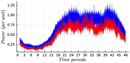
Figure 1. Stochastic behavior of the active and reactive power consumption at a specific power system substation, analyzed with a 30-min resolution, resulting in 48 time periods per day. The blue lines represent the active power consumption, while the red lines correspond to the reactive power consumption. Each line illustrates individual scenarios over a typical year.

This research employed uniform distributions to model variations in load demands and generation outputs within the power system. This approach was based on the understanding that operating conditions can vary widely while remaining constrained within defined limits. By employing uniform distributions, our work aimed to capture the full range of potential fluctuations that may occur in real-world scenarios [25,26]. This simplification is particularly useful for initial estimations, as it allows for performance analyses across a broad spectrum of conditions without overcomplicating the model. It should be noted that, while uniform distributions facilitate a clear representation of uncertainty, it is important to analyze their effects on the estimation of power losses and the reliability of the resulting B-coefficients, thereby ensuring that our methodology remains robust under various operating conditions [27].

To implement the general random generation approach, the primary tool is a power flow solver, which, in our proposal, is based on the classical NR technique available in MATLAB’s MATPOWER version 8.1. This tool is used to generate a wide range of operational scenarios for a specific power system while requiring only the minimum necessary data [28]. For each operating condition, the power flow is solved, and the calculated power losses are stored, effectively simulating the data obtained from the PMUs. Figure 2 illustrates this data-driven generation process using recursive power flow solutions across different operating conditions [5].

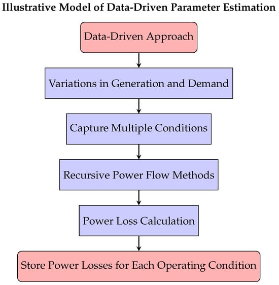
Figure 2. Flowchart illustrating the data-driven approach for estimating power losses through variations in generation and demand using recursive power flow methods.

The proposed solution methodology integrates a data-driven approach with two convex optimization models, i.e., LP and QP formulations. The primary objective is to compare the impact of each formulation on the expected B-coefficients. A summary of this approach is depicted in Figure 3.

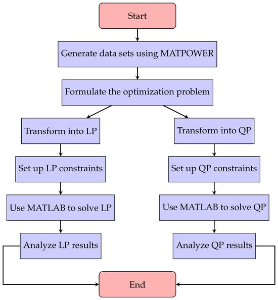
Figure 3. Flowchart for solving the optimization problem using convex tools in MATLAB. Branches for the LP and QP approaches are shown.

This flowchart provides a clear overview of our structured proposal for estimating B-coefficients. Starting from the generation of data sets using MATPOWER, this approach formulates the optimization problem tailored for both LP and QP models. Each branch outlines the steps for setting up the constraints, solving the optimizations in MATLAB, and analyzing the results, ultimately aiming to enhance the accuracy of B-coefficients estimation. This systematic method allows for a comprehensive comparison of the LP and QP models, ensuring that the selected methodology effectively addresses the complexities of power systems operation.

The proposed LP and QP formulations fundamentally differ from existing approaches, particularly in their specific focus on effectively capturing the nonlinear relationships between power generation and transmission losses through a quadratic objective function in the QP formulation. This capability enhances accuracy in parameter estimation while adeptly managing the complexities and stochastic nature of power systems operation. Furthermore, the LP and QP formulations uniquely incorporate essential physical constraints, ensuring that the estimated B-coefficients are both realistic and applicable within the context of operation. This integration allows for more precise and reliable estimations under varying conditions, addressing the challenges that are often encountered with traditional SDP approaches, which may impose overly restrictive constraints and struggle to adapt to real-world variability.

4. Numerical Validations

The performance of the proposed optimization model was evaluated using the IEEE 14-, 39-, 57-, and 118-bus test systems, which are detailed in [29,30,31]. A comparative analysis was conducted against the model presented in Equation (2). For each test system, $\mathbf{M}$ scenarios were generated, with the generator outputs randomly perturbed within 50% to 100% of their nominal capacities. Concurrently, the load demands were randomly varied between 40% and 100% of the nominal values. These adjustment ranges were selected to represent the typical variability encountered in power systems [32]. All simulations were performed using MATPOWER version 8.1 within MATLAB 2025b, via YALMIP interfaced with the MOSEK solver [33]. Additionally, the proposed models were compared to the deviation model proposed in [15], which is based on the quadratic Taylor series expansion.

Figure 4 shows the percent estimation errors obtained for 1000 randomly generated operational scenarios in the IEEE 14-, 39-, 57-, and 118-bus test systems. The left column corresponds to the deviation model, whereas the right column compares the LP and QP formulations. From this figure, the following observations can be made:

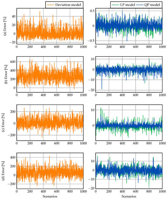
Figure 4. Estimation errors for the deviation model (left column) and the LP and QP models (right column): (a) IEEE 14-bus test system, (b) IEEE 39-bus test system, (c) IEEE 57-bus test system, and (d) IEEE 118-bus test system.

• For the 14-bus system (Figure 4a), the deviation model exhibits errors that approximately range between −20% and 45%, implying significant dispersion and a lack of consistency. In contrast, the LP and QP models maintain a performance similar: within an interval of $[-0.4\%,0.4\%]$, with small fluctuations across all scenarios.
• In the IEEE 39-bus system, the deviation model shows increased inaccuracy, with errors spanning roughly from 0% up to 600% and an average error of 266.2786% (Figure 4b). This indicates an increase in error estimation as the system size grows. Meanwhile, both the LP and QP models exhibit estimation errors around −10% and 6%, with the vast majority of estimates close to zero. This behavior is corroborated by their mean errors: −0.4086% and −0.3577% for the LP and QP models, respectively. Although the error range increases in comparison with the 14-bus case, the optimization models still maintain an acceptable performance—even when dealing with medium-sized networks.
• For the 57- and 117-bus systems, the deviation model continues to show large oscillations, with errors ranging approximately from −200% to 200% (Figure 4c,d). Meanwhile, the LP and QP models maintain errors between −12% and 12%. This demonstrates the consistency of our optimization-based models, which remain reliable even in large scale operations.

The average, minimum, maximum values of the estimation errors, as well as the first and third quartiles, are presented in Figure 5, aiming to quantify the performance of the deviation, LP, and QP models. The results illustrated in this figure allow for the following statements:

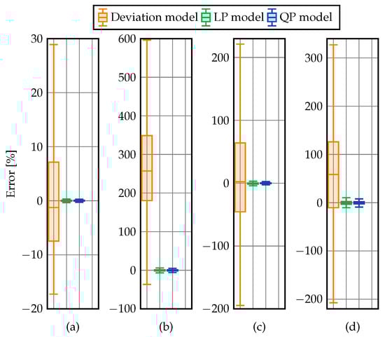
Figure 5. Average, minimum, maximum, first-quartile (top of the box), and third-quartile (bottom of the box) estimation errors: (a) IEEE 14-bus test system, (b) IEEE 39-bus test system, (c) IEEE 57-bus test system, and (d) IEEE 118-bus test system.

• In the 14-bus test system, the deviation model exhibits a very wide dispersion, with its interquartile range (IQR) roughly extending from −10% to 8%, as well as with an average estimation error close to 1% (Figure 5a). In contrast, the LP and QP models show a tighter clustering: their IQRs remain approximately between −0.25% and 0.35%, with mean errors around 0.03% for LP and 0.05% for QP. These results confirm that both optimization-based methods significantly outperform the deviation model in small systems.
• In the 39-bus test system, the deviation model becomes less reliable, showing an IQR approximately between 90% and 300%. On the other hand, the LP and QP models maintain their estimation accuracy, with their IQRs contained between −3% and 2%. Despite the increase in system complexity, both optimized formulations preserve their strong predictive performance.
• As for the 57- and 118-bus systems, the results reveal similar performance trends. The deviation model again exhibits a very large dispersion, with the IQRs spanning approximately from −100% to 80% (57-bus feeder) and from −120% to 90% (118-bus grid). Moreover, the average errors are around −15% and −18%, respectively. Conversely, the LP and QP models show tightly grouped errors, with the first–third quartiles ranging roughly from −1.2% to 1.0% for both systems. Their mean errors remain close to zero, ranging from −0.25 % to 0.20 %. This demonstrates that the optimization-based methods preserve accuracy even in large-scale networks.

Comparison of LP and QP Models

This section presents a MATLAB evaluation of the proposed LP and QP models’ performance in three large test systems comprising 200 (ACTIVSg200), 300 (IEEE 300-bus feeder), and 500 (ACTIVSg500) nodes. These test systems were selected because they represent increasingly complex transmission grids with diverse topological characteristics.

Figure 6 presents the percent estimation errors obtained from 10,000 randomly generated operational scenarios for the aforementioned test systems using both the LP and QP models. The figure also shows some statistical indicators, i.e., the average, minimum, and maximum values together with the first and third quartiles, providing a comprehensive view of our proposal’s estimation performance across a wide range of operating conditions.

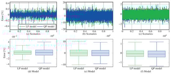
Figure 6. Estimation errors for (left column) and their statistical values (right column): (a,d) 200-bus test system; (b,e) 300-bus test system; (c,f) 500-bus test system.

From Figure 6, it can be stated that

• For the 200-bus system, both models exhibit small and bounded errors, with values below 0.5% in most scenarios. The QP model shows a slightly higher dispersion than the LP model (Figure 6d).
• In the 300-bus test system, both models show noticeably larger variability than in the 200-bus feeder, with a deviation of approximately $\pm 10\%$. Nevertheless, Figure 6e shows that more than 50% of the scenarios exhibit estimation errors below 2%. This indicates that the majority of operating conditions are well captured despite the increased nonlinearities of this medium-sized network.
• As for the 500-bus system, both models achieve significantly reduced percent errors compared to the 300-bus case, suggesting that the relative loss magnitudes scale more favorably with system size in this synthetic grid.

Table 1 summarizes the numerical performance of the LP and QP models across the seven test systems analyzed in this study. This table reports three key indicators: computation time, average percent error, and the standard deviation of the estimation error based on 10,000 operational scenarios for each system.

Table 1. Comparison of the performance of the LP and QP models.

Bus	${\mathbf{N}}_{\mathbf{g}}$	Computation Time [s]		Average Error [%]		Std. Deviation [%]
		LP	QP	LP	QP	LP	QP
14	3	0.2928	0.2160	−0.0011	0.0167	0.1420	0.1263
39	10	0.8591	0.4547	0.1705	−0.1896	1.5751	1.5920
57	7	0.5082	0.3140	−0.4934	−0.4650	2.1220	1.8562
118	54	26.5811	14.6094	−0.2084	−0.1485	3.3206	2.9559
200	38	7.4315	3.0726	0.0019	0.0002	0.0387	0.0329
300	69	52.1159	27.2672	−0.1027	−0.0594	3.9342	3.5895
500	56	42.0950	20.8765	−0.0783	−0.1143	0.4680	0.4889

In Table 1, note that

• The computational burden of the QP model remains manageable. Although the QP formulation requires more computational resources than the LP model, the differences in runtime become proportionally smaller as system size increases. For instance, in the 300- and 500-bus systems, the QP model is approximately twice as fast as the LP model, highlighting its favorable scalability and practical suitability for large-scale applications.
• The QP model outperforms its LP counterpart in terms of estimation accuracy. For all systems, the QP formulation yields lower average errors and reduced standard deviations, confirming its superior ability to capture the nonlinear dependence of transmission losses on power flows. This better performance is evident in medium-sized networks such as the 57- and 118-bus systems, where the LP model exhibits larger deviations due to increased nonlinear interactions.
• The estimation variability decreases in the largest synthetic systems (i.e., the 200-, 300-, and 500-bus feeders); the percent errors diminish as absolute transmission losses scale with network size. Even in these cases, the QP model maintains a lower dispersion and more tightly bounded error distributions.

Overall, Table 1 demonstrates that the QP model strikes a favorable balance between accuracy and computational efficiency, providing more reliable loss estimates than the LP model across all the evaluated test systems.

5. Conclusions and Future Works

This study presented a novel approach for estimating transmission loss coefficients, specifically B-coefficients, by integrating LP and QP models within a data-driven methodology. The results demonstrated that both LP and QP formulations significantly enhance the accuracy and reliability of B-coefficient estimates compared to traditional methods. The proposed models achieved estimation errors averaging less than 3.5% across various operational scenarios using IEEE test systems, showcasing notable improvements over existing estimation techniques.

By leveraging simulated measurement data that reflected the stochastic nature of power generation and demand, the proposed models effectively captured the complex behaviors associated with power losses in transmission networks. This approach enabled the incorporation of a wide range of operating conditions, ensuring that the resulting estimates were robust and relevant. Additionally, while both LP and QP are convex optimization frameworks, their ability to address parameter identification problems without depending solely on gradient information greatly enhances their applicability in real-world scenarios.

Our findings underscore the importance of accurate B-coefficient estimation, not only for immediate operational decisions, but also for long-term planning and sustainability. Reliable coefficients enable system operators to better predict transmission losses, yielding lower operating costs and supporting the integration of renewable energy sources, which is critical for enhancing the reliability and resilience of modern power systems.

Looking ahead, future research should prioritize refining the proposed estimation techniques by integrating real-time data inputs from PMUs and other advanced monitoring technologies. This integration could significantly enhance the adaptability of our models to dynamic changes in power system conditions, resulting in even more accurate and timely B-coefficients estimates. Furthermore, exploring the application of machine learning algorithms alongside the LP and QP models may further improve estimation accuracy, particularly in scenarios characterized by high uncertainty and variability.

Moreover, future studies could investigate the scalability of the proposed approach in larger and more complex power systems. Addressing the challenges associated with integrating variable renewable energy sources remains a key research area. Effectively modeling and estimating B-coefficients while dealing with the inherent variability of renewable generation is crucial for optimizing power system performance and promoting sustainable energy practices. Ultimately, these advancements could contribute to developing more efficient and resilient power grid management strategies, further supporting the transition towards greener energy solutions.

References

- Motta, V.N.; Anjos, M.F.; Gendreau, M. Survey of optimization models for power system operation and expansion planning with demand response. Eur. J. Oper. Res. 2024, 312, 401–412. [Google Scholar] [CrossRef]
- Maghami, M.R.; Yaghoubi, E.; Mohamed, M.; Yaghoubi, E.; Jahromi, M.Z.; Fei, T.K. Multi-objective optimization of unbalanced power distribution systems: A comprehensive approach to address uncertainties and enhance performance. Energy Convers. Manag. X 2025, 27, 101087. [Google Scholar] [CrossRef]
- Liu, B.; Liu, F.; Wei, W.; Wang, J. Estimating B-coefficients of power loss formula considering volatile power injections: An enhanced least square approach. IET Gener. Transm. Distrib. 2018, 12, 2854–2860. [Google Scholar] [CrossRef]
- Zarco, P.; Exposito, A. Power system parameter estimation: A survey. IEEE Trans. Power Syst. 2000, 15, 216–222. [Google Scholar] [CrossRef]
- Montoya, O.D.; Gil-González, W. Accurate measurement-based convex model to estimate transmission loss coefficients in power systems. Electr. Power Syst. Res. 2024, 237, 111036. [Google Scholar] [CrossRef]
- Cárdenas Guerra, C.A.; Ospino Castro, A.J.; Peña Gallardo, R. Analysis of the Impact of Integrating Variable Renewable Energy into the Power System in the Colombian Caribbean Region. Energies 2023, 16, 7260. [Google Scholar] [CrossRef]
- Kunya, A.B.; Abubakar, A.S.; Yusuf, S.S. Review of economic dispatch in multi-area power system: State-of-the-art and future prospective. Electr. Power Syst. Res. 2023, 217, 109089. [Google Scholar] [CrossRef]
- Talbi, E.H.; Abaali, L.; Skouri, R.; Moudden, M.E. Solution of Economic and Environmental Power Dispatch Problem of an Electrical Power System using BFGS-AL Algorithm. Procedia Comput. Sci. 2020, 170, 857–862. [Google Scholar] [CrossRef]
- Raharjo, R.M.; Sarjiya, S.; Wijaya, F.D.; Multa Putranto, L.; Yasirroni, M. Improved Kron Method for Linear Losses Coefficient. In Proceedings of the 2023 IEEE International Conference on Advanced Mechatronics, Intelligent Manufacture and Industrial Automation (ICAMIMIA), Lombok, Indonesia, 14–15 November 2023; pp. 352–357. [Google Scholar] [CrossRef]
- Bretas, A.S.; Rossoni, A.; Trevizan, R.D.; Bretas, N.G. Distribution networks nontechnical power loss estimation: A hybrid data-driven physics model-based framework. Electr. Power Syst. Res. 2020, 186, 106397. [Google Scholar] [CrossRef]
- Gharehchopogh, F.S.; Maleki, I.; Dizaji, Z.A. Chaotic vortex search algorithm: Metaheuristic algorithm for feature selection. Evol. Intell. 2021, 15, 1777–1808. [Google Scholar] [CrossRef]
- Bertozzi, O.; Chamorro, H.R.; Gomez-Diaz, E.O.; Chong, M.S.; Ahmed, S. Application of data-driven methods in power systems analysis and control. IET Energy Syst. Integr. 2023, 6, 197–212. [Google Scholar] [CrossRef]
- Happ, H.H.; Hohenstein, J.F.; Kirchmayer, L.K.; Stagg, G.W. Direct Calculation of Transmission Loss Formula-II. IEEE Trans. Power Appar. Syst. 1964, 83, 702–707. [Google Scholar] [CrossRef]
- Fliscounakis, S.; Lafeuillade, F.; Limousin, C. Estimation of transmission loss coefficients from measurements. In Proceedings of the 2005 IEEE Russia Power Tech, St. Petersburg, Russia, 27–30 June 2005. [Google Scholar] [CrossRef]
- Huang, W.T.; Yao, K.C.; Chen, M.K.; Wang, F.Y.; Zhu, C.H.; Chang, Y.R.; Lee, Y.D.; Ho, Y.H. Derivation and Application of a New Transmission Loss Formula for Power System Economic Dispatch. Energies 2018, 11, 417. [Google Scholar] [CrossRef]
- Chang, Y.C.; Yang, W.T.; Liu, C.C. A new method for calculating loss coefficients of power systems. IEEE Trans. Power Syst. 1994, 9, 1665–1671. [Google Scholar] [CrossRef]
- Alshawawreh, J.A. Power Losses Formula for Optimal Power Flow Problem in Power System. Int. J. Appl. Eng. Res. 2018, 13, 2471–2476. [Google Scholar]
- Alwan, S.H.; Razzaq Altahir, A.A.; Al Tu’ma, A.S. Calculations of Loss Factor Based on Real-Time Data: Determining Technical Power Loss for the Electrical Distribution Network in Karbala City. IOP Conf. Ser. Mater. Sci. Eng. 2020, 671, 012037. [Google Scholar] [CrossRef]
- Jethmalani, C.H.R.; Dumpa, P.; Simon, S.P.; Sundareswaran, K. Transmission Loss Calculation using A and B Loss Coefficients in Dynamic Economic Dispatch Problem. Int. J. Emerg. Electr. Power Syst. 2016, 17, 205–216. [Google Scholar] [CrossRef]
- Ram Jethmalani, C.; Simon, S.P.; Sundareswaran, K.; Srinivasa Rao Nayak, P.; Padhy, N.P. Real coded genetic algorithm based transmission system loss estimation in dynamic economic dispatch problem. Alex. Eng. J. 2018, 57, 3535–3547. [Google Scholar] [CrossRef]
- Asghari, M.; Fathollahi-Fard, A.M.; Mirzapour Al-e hashem, S.M.J.; Dulebenets, M.A. Transformation and Linearization Techniques in Optimization: A State-of-the-Art Survey. Mathematics 2022, 10, 283. [Google Scholar] [CrossRef]
- Hladík, M.; Moosaei, H.; Hashemi, F.; Ketabchi, S.; Pardalos, P.M. An overview of absolute value equations: From theory to solution methods and challenges. Comput. Optim. Appl. 2025, 93, 435–488. [Google Scholar] [CrossRef]
- Martin, R.K. Large Scale Linear and Integer Optimization: A Unified Approach; Springer: New York, NY, USA, 1999. [Google Scholar] [CrossRef]
- Dostál, Z. Optimal Quadratic Programming and QCQP Algorithms with Applications; Springer Nature: Cham, Switzerland, 2025. [Google Scholar] [CrossRef]
- Megantoro, P.; Halim, S.A.; Kamari, N.A.M.; Awalin, L.J.; Ali, M.S.; Rosli, H.M. Optimizing reactive power dispatch with metaheuristic algorithms: A review of renewable distributed generation integration with intermittency considerations. Energy Rep. 2025, 13, 397–423. [Google Scholar] [CrossRef]
- Tian, Z.; Deng, W.; Liu, M.; Lv, L.; Chen, Z. Empowering Sustainability in Power Grids: A Multi-Scale Adaptive Load Forecasting Framework with Expert Collaboration. Sustainability 2025, 17, 10434. [Google Scholar] [CrossRef]
- Hakami, A.M.; Hasan, K.N.; Alzubaidi, M.; Datta, M. A Review of Uncertainty Modelling Techniques for Probabilistic Stability Analysis of Renewable-Rich Power Systems. Energies 2022, 16, 112. [Google Scholar] [CrossRef]
- Guerra, G.; Martinez-Velasco, J.A. Evaluation of MATPOWER and OpenDSS load flow calculations in power systems using parallel computing. J. Eng. 2017, 2017, 195–204. [Google Scholar] [CrossRef]
- Liu, X.; Zhang, T. Analysis of IEEE 14 bus power flow calculation characteristics based on Newton-Raphson method. In Proceedings of the 2022 IEEE 5th International Conference on Automation, Electronics and Electrical Engineering (AUTEEE), Shenyang, China, 18–20 November 2022; pp. 1092–1097. [Google Scholar] [CrossRef]
- Chen, K.; Tie, Y.; Li, M. Importance Evaluation of Power Grid Transmission Lines Based on Multidimensional Information Feature Mapping. Energies 2024, 17, 6013. [Google Scholar] [CrossRef]
- Alanazi, A.; Alanazi, M.; Memon, Z.A.; Mosavi, A. Determining Optimal Power Flow Solutions Using New Adaptive Gaussian TLBO Method. Appl. Sci. 2022, 12, 7959. [Google Scholar] [CrossRef]
- Almutairi, A.; Ahmed, M.H.; Salama, M. Probabilistic generating capacity adequacy evaluation: Research roadmap. Electr. Power Syst. Res. 2015, 129, 83–93. [Google Scholar] [CrossRef]
- Löfberg, J. YALMIP: A Toolbox for Modeling and Optimization in MATLAB. In Proceedings of the 2004 IEEE International Conference on Robotics and Automation (IEEE Cat. No.04CH37508), Taipei, Taiwan, 2–4 September 2004; pp. 284–289. [Google Scholar] [CrossRef]
Disclaimer/Publisher’s Note: The statements, opinions and data contained in all publications are solely those of the individual author(s) and contributor(s) and not of MDPI and/or the editor(s). MDPI and/or the editor(s) disclaim responsibility for any injury to people or property resulting from any ideas, methods, instructions or products referred to in the content. |
© 2026 by the authors. Licensee MDPI, Basel, Switzerland. This article is an open access article distributed under the terms and conditions of the Creative Commons Attribution (CC BY) license.