


Abstract
Compared to the façades of student multi-story dormitories, flat horizontal roofs offer greater freedom in shaping the layout, orientation, horizontal inclination, and geometry of photovoltaic installations (PVI). The large number of parameters defining the geometric and physical characteristics of PVI necessitates the development of a method to support the optimization of energy renovation processes. To facilitate this innovative method, several automation and optimization procedures were implemented into a specialized computer application developed within the Rhino/Grasshopper graphical programming environment. The method’s algorithm allows for the definition of an initial parametric qualitative model of each rooftop installation. This model is configured through multiple iterative computer simulations aimed at identifying various discrete optimal qualitative models. The implemented optimizing condition concerns the amount of energy produced and relates to the variability of energy prices as well as the costs of purchasing and mounting the PVI. The optimizing procedure involves replacing a specific portion of grid energy with electricity produced by the PVI. The parameters describing variability include the geometric and physical properties, as well as the orientation of the PVI. In the second step, the algorithm optimizes the desired payback period and investment costs. The obtained results fill a gap in the field of multi-parameter optimizing methods for the energy renovation of student dormitories.
1. Introduction to Student Dormitory Renovations
1.1. Justification for Taking up the Topic
In the temperate climate of the Central European Plain, energy supplied to a building is used for external and internal equipment, heating the interior during cool and cold seasons (spring, autumn, and winter), and cooling during the hot season (summer) [1]. The grid energy supplied to meet various operational needs of the building and its occupants can be fully or partially replaced by electricity produced by photovoltaic installations (PVI), depending on the building’s functions and investment costs. In the case of student dormitories, there is a need to supply a large amount of electricity due to the constant requirements resulting from the permanent residence of a significant number of people around the clock. These needs remain relatively constant and change little throughout the year [2].
Therefore, it is justified to utilize solar energy to produce electricity to replace a significant portion of the grid energy supplied to student dormitories. Central Europe’s solar potential is sufficient to replace a large portion of the grid-sourced energy for eight to nine months during the warm seasons to fulfill these needs [3]. During the two or three cold months (December, January, and February), the electricity produced by a reasonable number of PV panels is low and significantly inadequate for the actual needs of dormitory residents. Considering the annual replacement rates of grid-sourced electricity with energy produced by PVI, it is advisable to target a replacement rate of 70–85%, accounting for a slight surplus of electricity production in summer and insufficient production in winter.
The primary goal is, therefore, to develop a method for the energy renovation of dormitories using PVI to produce an optimal amount of electricity. Since the payback period and investment costs depend on many factors—including the layout, orientation, azimuth, tilt, size, efficiency, and costs of the installed PV panels—parametric analysis and methods based on computer calculations using artificial intelligence are becoming increasingly important [4].
1.2. Critical Analysis
The effectiveness of building renovations with integrated PV panels largely depends on solar potential of the regions where the modernized buildings are located. M. Suri et al. [5] analyzed the solar potential of Central Europe. They developed a method for determining solar irradiance of this area, based on a geographical information system called GIS. They showed that the solar potential varies from 850 kWh/m2 for the northern zones to 1050 kWh/m2 for the southern ones.
D. Buchalova et al. [6] developed an analogous parametric GIS-based method for determining the solar potential of building envelopes, which is applicable for technical purposes. An analogous, more general method for determining the solar potential of differently oriented and inclined planes was elaborated by R. Mueller et al. [7]. This method can also be employed to calculate the solar potential of PV panels arranged on building envelopes (roofs and facades). Based on this method, online tools recommended by the European Commission for calculating the solar potential of buildings were developed [8].
Solar potential of various geographical zones, building envelopes, and PV panels depends on the type and magnitude of solar radiation hitting their surfaces. It is primarily influenced by the amount of direct solar radiation that varies depending on the time of day and the year [9]. Diffuse solar radiation is another type of solar radiation that has a lesser effect on the solar potential of PV panels; however, this effect is still significant. The direct and diffuse solar radiation vary throughout the day and the year because of the Earth’s rotation around its axis and around the Sun and the transparency and cloud cover of the northern hemisphere [10].
P.U. Poornima et al. [11] examined the economic feasibility and energy efficiency of rooftop vertical and horizontal photovoltaic installations in subtropical zones using Quantum Particle Swarm Optimization, Q-Learning System, and MATLAB (version 2022a) dynamic simulations. Their research resulted in methods optimizing the costs of electricity, lifespan, performance ratio, and carbon footprint. They found that optimal solutions in equatorial locations are less organized arrangements, while those in non-equatorial areas are based on single-azimuth rows. A. Barman et al. [12] analyzed the energy production of PVIs arranged on horizontal and vertical planes of residential high-rise building envelopes localized to monsoon tropical zones. Their research revealed that the electricity production by the panels arranged on vertical façades (southern, eastern, or western ones) was about 49% higher compared to the panels distributed on horizontal roofs.
S. I. Kaitouni et al. [13] analyzed the solar potential of tall buildings and their energy-driven optimization in various scenarios typical of the Mediterranean climate. They developed a parametric method of determining energy-effective buildings integrated with PVI based on two geometric variables. These were a shape factor and an orientation of buildings. The authors concluded that PVI can enhance the daily load cover factor and lead to an improvement of the renovated buildings up to 12.4%. A parametric method of determining the solar potential of building envelopes located in a temperate climate was elaborated by J. Abramczyk and W. Bielak [14].
N. Aste et al. [15] developed new energy models of roofs and buildings operating in diverse meteorological zones, from Mediterranean to Nordic, including Oceanic and Continental. The authors simulated the shape, tilt, and azimuth angles of the investigated envelope’s elements and PVI. They employed PVI to obtain the net-zero energy target in residential multi-story buildings. Their basic conclusion is that PVI can yield net zero energy buildings for 1.3 story in Nordic climate and 2.0 stories in Continental/Oceanic, while in the Mediterranean it can achieve almost 3.0 stories. They also discussed the optimal angle of inclination of PV modules, which should be equal to the latitude of the examined sites minus 10° to 15°.
A. Young-Sub et al. [16] analyzed various renovations of tall buildings with PVI distributed on vertical facades and pitched or horizontal roofs in humid tropical monsoon zones. They found that the renewable energy generation rates are 2.48 to 2.75 times higher when using building integrated PVIs. In the examined cases, the annual renewable energy sharing rates increased from 58.9% to 146.2%.
A. Kazemian and C. Xiang [17] analyzed PVT-green roofs and their thermal, electrical, and structural synergies to transition the examined theoretical models into practical applications. They advocated for the empirical research to validate and optimize their models. They presented three critical barriers: high initial costs, climate-specific performance variability, and structural integration limitations crucial in the renovation process.
T. Paphapote et al. [18] accomplished many optimizing processes related to an impact of the inclination, shading, and inter-row spacing of floating photovoltaics on the energy use of various buildings located in tropical monsoon zones. Their optimized configurations were characterized by a 6° azimuth and 1.00 m inter-row spacing. Their study was based on dynamic simulations, hourly meteorological data, PVsyst 7.4 software, and analytical methods.
V. Shekar et al. [19] presented a three-dimensional method of determining the optimal azimuths for building-integrated PVI in the Arctic. The method employs dynamic computer simulations to minimize energy consumption and economic costs in Finland. The authors analyzed several building types with various dimensions and roof sizes, equipped with panels of different surface areas. They found that a PVI azimuth in the 70–270° range results in a 3% discount rate, while an azimuth in the 120–200° range results in a 5% discount rate.
A. Ahmed et al. [20] analyzed various parametric characteristics of PVI arranged on the roofs of buildings located in different zones. The modeled villas and apartments offered 30% and 21% rooftop usability for PVI, respectively. They found that PVI can offset 15% to 87% of the total grid load, while the cooling load can be reduced by 4.5%, and the interest rate for life cycle cost can reach 22%. H. Wu et al. [21] developed a parametric method of renovating typical high-rise residential buildings with PVI taking into account economic costs and employing the NSGA-II genetic algorithm to achieve optimal solutions. Their results showed that the replacement rates of grid energy with electricity produced by PVI range from 70% to 90% in cool areas of China; however, in cold regions, these rates range from 35% to 50%. L. Tao et al. [22] employed the Random Forest algorithm and genetic algorithms to optimize PVI electricity generation, achieving a level of 56 kWh/m2, which led to an eight-and-a-half-year payback period.
P. Movahhed et al. [23] conducted research on energy generation by PV-green and PV-cool roofs as well as building energy consumption. B. Mauer et al. [24] also analyzed the energy operation of roofs with PVI integrated into green and cool coverings.
J. Abramczyk and W. Bielak [2] presented a parametric, automated method for renovating multi-story student dormitories integrated with PV installations distributed on their façades. Several novel parametric and discrete models were developed to perform many simulations and energy optimizations of the PVIs. The authors conducted a parametric analysis of the payback period based on grid energy replacement rates and costs. A discrete, optimal quantitative model for dormitory modernization was the result of each optimizing process. A payback period of 79 months and an 0.434 energy replacement rate of 0.434 were calculated. The volume of each examined building was 17,800 m3, while the annual energy produced by PVI amounted to 68,500 kWh. The calculations were based on a real-world modernization of the IKAR student dormitory located in Rzeszów, located in the Central European Plain, and took into account the guidelines published by the European Commission [8]. The configured models were then employed in the present research related to simulations of roof-integrated PVIs.
Based on the above review, the following gaps in current knowledge were identified. There is a need to develop a parametric method for the energy renovations of multi-story student dormitories using different rooftop PVI models. This method should be based on qualitative input and output models, optimized and validated for the temperate climate conditions of Central Europe.
It seems advisable to automate the energy optimizing process for renovating multi-story student dormitories to obtain an optimal solution. This guarantees investors that their expectations regarding costs, payback periods and replacement rates are met. The developed automation, parameterization and optimization can facilitate the use of this method in technical applications. The method can support the search for efficient and optimal solutions. It is also advisable to create qualitative output models leading to individual optimal solutions under various optimizing conditions.
1.3. The Aim
The aim is to present the algorithm of a novel parametric method for renovating multi-story student dormitories with rooftop PVI to replace energy supplied via external networks. The algorithm is based on a new parametric strategy employing several qualitative input and output models defined by the geometric, energy, and cost characteristics of the designed PVI. These parametric models are used to generate a series of discrete models for computer simulations. The simulations were performed to investigate the relationships occurring during electricity production by the PVI. These parametric models were implemented in the Rhino/Grasshopper computer environment to simulate the energy performance, pricing, operation, and costs of the PVI.
Each optimizing process results in a single optimal PVI model, characterized by energy-efficient operation based on the solar irradiance of its panels. Thus, the algorithm uses each parametric input model to optimize the solar potential of the PVI when replacing grid energy. In this step, three out of eight input parameters (independent variables) were optimized: the azimuth, the tilt angle, and the spacing between subsequent rows of PV panels.
Next, a parametric qualitative output model is used to determine the payback period, costs of PVI, and the annual profits resulting from the reduction in an arbitrary part of grid energy consumption. The discrete models obtained in the final step of the calculations allow for the identification of several key relationships between independent and dependent variables.
The developed method for finding optimal solutions is fully automated; therefore, it is highly accessible to designers. It is supported by a novel computer application that simulates the natural environment, the energy performance of PV panels, and the genetic algorithms leading to optimal solutions. Future studies are planned to explore various types of renovations and various optimizing conditions. The currently proposed discrete and parametric models can be easily modified to include additional independent and dependent variables, enabling the definition of new renovation types and the generation of alternative solutions.
2. Methodology
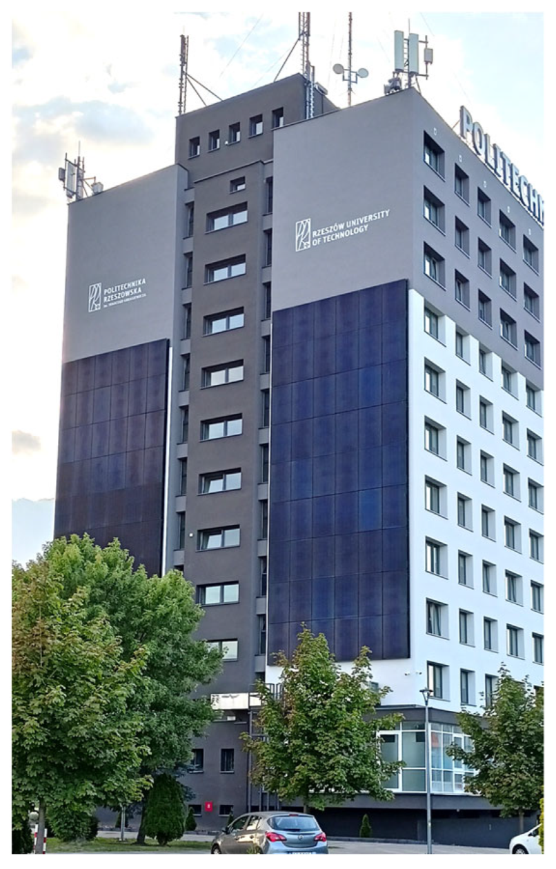
The algorithm of the developed method supports the renovation of various types of multi-story rectangular student dormitories, including the example shown in Figure 1. This dormitory serves as the reference model for the further analysis presented in the following sections. The discrete models employed in the performed simulations were configured based on the analysis by J. Abramczyk and W. Bielak [2], which concerned PVIs integrated into the facades of the same IKAR student dormitory. The designed renovations were supported by several parametric models utilized during simulations accomplished in the Rhino/Grasshopper visual programming environment [25].
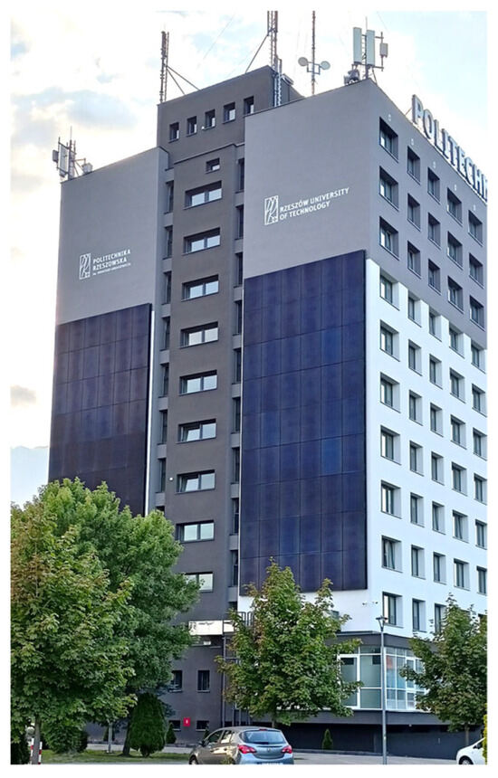
Figure 1.
The basic IKAR dormitory modernized with PVI.
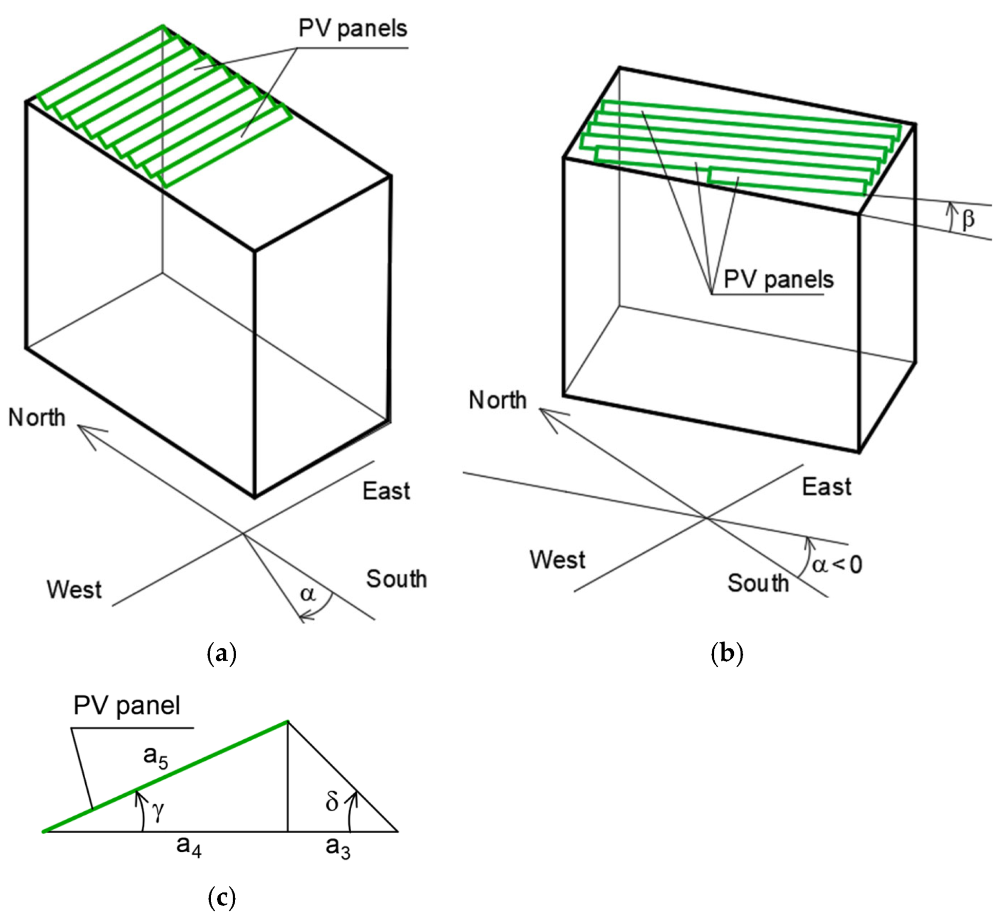
The first step of this algorithm involves creating a geometric parametric, and quantitative Mfpg model of dormitories with integrated PVI, as shown in Figure 2a,b. The designed PV panels are arranged on horizontal roofs and can be freely oriented. Eight input parameters, Xi, were adopted as independent variables. The first five variables are as follows: β—the angular difference between the azimuth of building and the azimuth of all PV panels, as shown in Figure 2b, γ—the angle of inclination of PV’s planes relative to the horizontal plane, as shown in Figure 2c, a5—the height of each PV panel (Figure 2c), Rat—the ratio of the surface area of all PV planes to the roof surface area, δ—the angle defining the a3 distance between adjacent rows of PVI, as shown in Figure 2c.
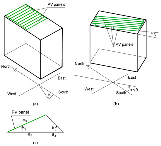
Figure 2.
Two parametric models of a multi-story student residence hall modernized with PVI distributed on a roof and (a) facing-south, (b) facing-south-east; and (c) A detail of inclination of PV panels to a horizontal plane.
The next three parameters, Rep, Prc, and Rcn, are also independent variables related to the economic aspects of the energy renovations. These include the Rep net energy replacement rates the substitution of grid energy by electricity produced by the PVI; the Prc price per 1 kWh net energy; and the Rcn ratio of renovation costs to net energy prices multiplied by 1000.
The values of the selected key coefficients used in the simulations are provided in Table 1. These include the dimensions, azimuth, geographic coordinates, and elevation above see level of the examined buildings, as well as the total energy Etot supplied to cover meet occupant needs (excluding energy allocated to HVAC systems). These coefficients, along with the assumed variation ranges of the input parameters Xi, shown in Table 2, constitute the boundary conditions for the calculations.

Table 1.
The characteristics of the real multi-story student dormitory and the designed PVI.
Table 2.
The ranges of the Xi independent variables defining the examined energy renovating processes related to the multi-story student residence hall.
The limit values of the ranges presented in Table 2 result from typical solutions adopted for buildings with integrated PVIs. For example, the azimuth range in the second column results from the 90° difference between the azimuths of two consecutive building façades and the possibility of adjusting them within a range of ±35°. Furthermore, changing the azimuths within a range of ±45° relative to the cardinal directions does not significantly affect the results compared to the ±35° for the analyzed geographical zone [3].
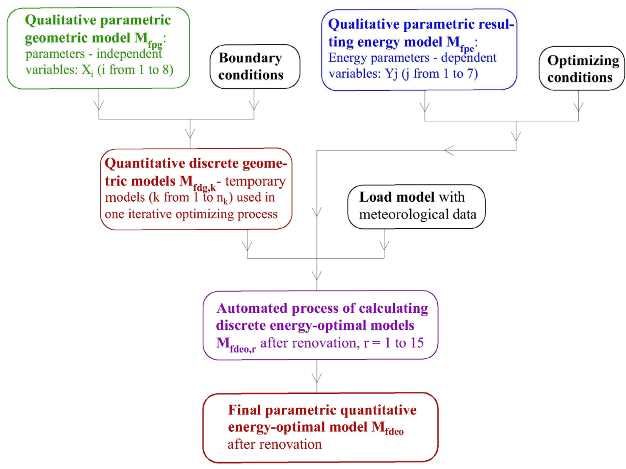
In the second step of the algorithm, discrete Mfdg,k models have to be constructed during each iterative k-th phase of the computer simulations to select the optimal Mfdeo,r model at the end of each r-th simulation process, as shown in Figure 3. A single Mfdg,k model is defined by adopting specific values for Xi. In particular, the values β, γ, and Rat are optimized in each single r-th computer simulation, which constitute a single r-iterative process. Thus, numerous temporary discrete Mfdg,k models are created in subsequent k-iterations based on the Mfpg model. Once the optimizing condition is met with the satisfactory accuracy, then the iterations are stopped, and all Mfdg,k models are compared to identify the optimal Mfdeo,r model. The Galapagos module employs a genetic algorithm to select the optimized Mfdeo,r solution.
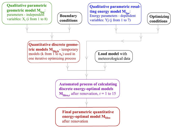
Figure 3.
The concept of the developed method of removing dormitories.
In the third step of the algorithm, several derivative computer simulations are executed to analyze the economic characteristics of energy renovations and to determine the effective Mfdeo model based on the previously created Mfdeo,r. In their research, twenty computer simulations (r = 1 to 20) were performed. Each r-th simulation is an iterative process leading to an energy-optimal solution, Mfdeo,r, defined by a set of seven dependent variables Yj (j = 1 to 7). These variables must be defined in the first step of the algorithm to formulate the simulation objectives. They include CTS—the costs of the PVI, PBK—the payback period of the renovation investment, TSP—the total surface area of the panels distributed on the roof, AOP—the roof area occupied by PV panels, COR—the total cost of constructing 1 m2 of PVI, AEL—the amount of electricity produced by the PVI, and RER—the net energy replacement rate, which define the cost of the net energy replaced by the electricity produced by the PV panels.
The optimizing condition related to the energy balances required by the method was defined as the equality between the amount of electricity produced by the PVI and the appropriate part of energy supplied by the power grid to serve the dormitory equipment, including lighting, computers, refrigerators, etc.
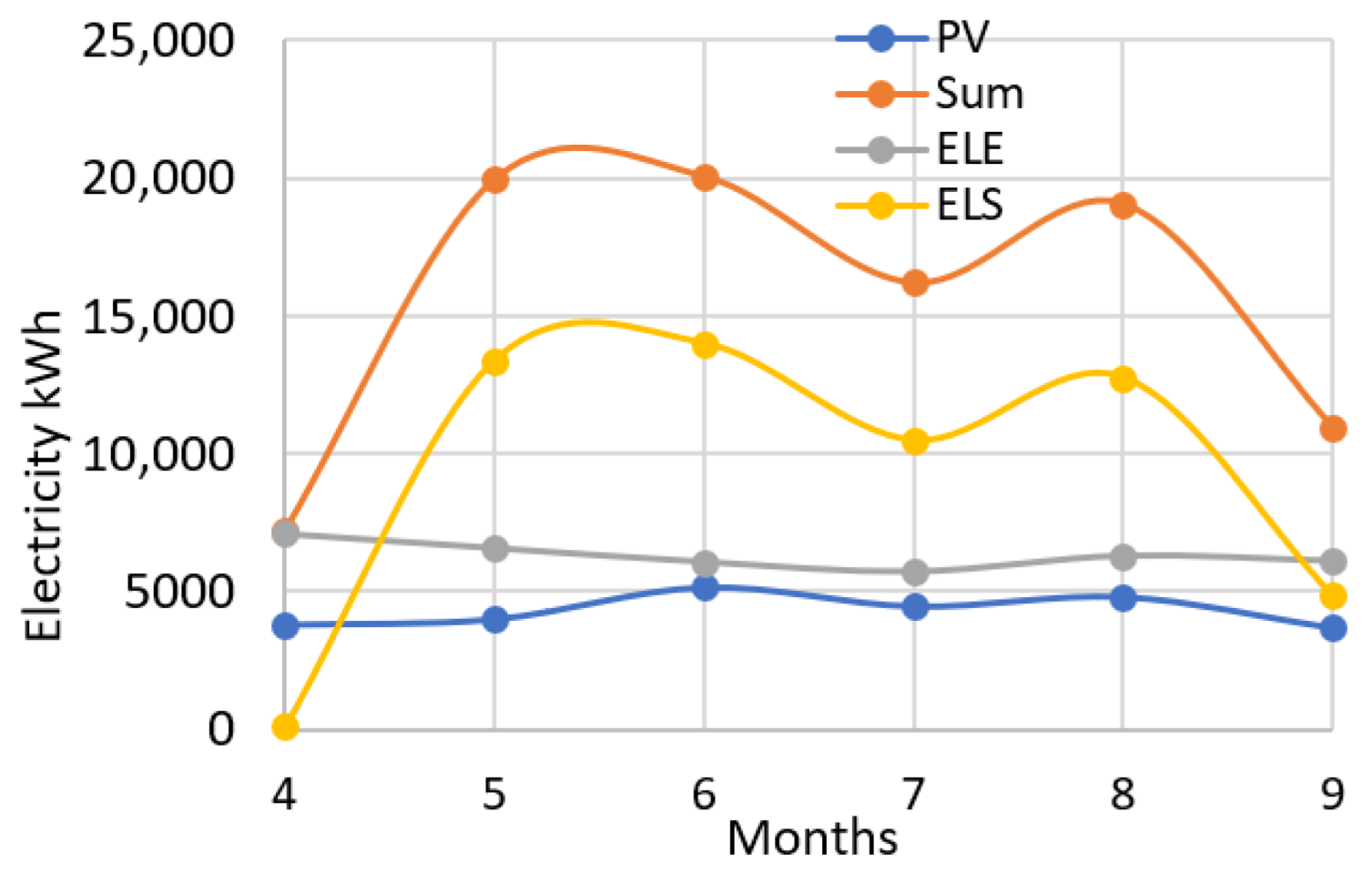
The diagram in Figure 4 presents the monthly electricity demands of the IKAR dormitory [2]. This building has 240 rooms (12 to 17 m2, 24 on each floor), which accommodate approximately 400 students. The ELE line represents the electricity demand of the student rooms, while the ELES line illustrates the demand of the service spaces, including the equipment of the gas heating system. The PV line describes the electricity produced by the PVI distributed on the south-eastern façade of the IKAR building from April 2025 to September 2025, totaling 23.5∙103 kWh over five months. These vertically arranged crystalline silicon PV panels have a capacity of 50 kWp, system losses of 14%, an angle of incidence up to 4°, and a total surface area of 250 m2 (comprising two large rectangles, as shown in Figure 1). In cases where the panels were well-maintained, the total losses did not exceed 23%.
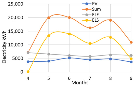
Figure 4.
The monthly electricity produced by the real PVI arranged on the east-south façade of the IKAR dormitory.
The amount of replaced grid energy Etot is determined by the Rep arbitrary energy replacement rates. These values are consistent with the characteristics of the actual modernization performed for the IKAR student residence hall, shown in Figure 1. Subsequently, the energy-optimized discrete models Mfdeo,r allow for an analysis of the relationships between the independent Xi variables and the dependent Yj variables. The amount of electricity produced per 1 m2 of PV panels is calculated based on the panel efficiency and solar irradiation data, which is downloaded from the referenced website [8] via an internal module of the proprietary application designed in the Rhino/Grasshopper.
It was also assumed that each optimization process is terminated once the required calculation accuracy is achieved regarding the substitution of grid energy Etot with the electricity AEL produced by the PV panels. The genetic algorithm within the Galapagos application is used to find the minimum value that satisfies the accuracy requirements of the optimizing condition, as defined in Equation (1).
Temporary values of AEL are calculated during each iterative loop of a single simulation. The final optimal value of AEL is calculated at the end of each optimizing processes. The values of AEL calculated for the twenty Mfdeo,r models are presented in detail in the next section. It was assumed that the square of the difference dEtot calculated for each optimizing condition (Equation (2)) must fall within the range defined by Equation (3).
The payback period PBK is calculated using Equation (4).
where PBK is measured in months. The costs CTS of PVI can be determined using Equation (5).
where TSP is calculated at the end of each optimization process. The annual cost RER of the part of net energy replaced by the energy AEL produced by the PVI can be calculated using Equation (6).
The condition limiting calculations and concerning roof area covered by PV panels was defined by Equation (7) related to the calculating accuracy and the surface area of PVI.
where AOP is the roof area covered by PV panels together with the areas between subsequent rows of PV panels resulting from the δ angle, see Figure 2c. Ab is the roof area calculated using Equation (8).
where a1 and a2 are the length and the width of roof.
3. Simulation Results
To obtain twenty discrete optimal models Mfdeo,r meeting the aforementioned specific initial conditions, twenty computer simulations (r = 1 to 20) were carried out. The main properties of these models are given in Table 3. The first column presents the symbols of the subsequent models employed in the simulations, which were defined by the parameters Xi (i = 1 to 8). As a result of each optimizing process, the values of three independent variables—β, γ, and Rat presented in the second, the third, and the fifth columns, respectively—were calculated. The values of a5 and δ as well as subsequent variables were kept constant in each optimizing process. The variables a5, δ, and Rep were adopted at three levels, with the middle value corresponding to the value used in the actual renovation of the IKAR dormitory.
Table 3.
The independent variables defining the Mfdeo,r models employed in the energy modernization processes of the real multi-story student residence hall.
The variation ranges of the independent variables Xi, presented in the subsequent columns of Table 3, were assumed to be consistent with typical values used in building renovations, taking into account the values adopted for the real-world renovation of the IKAR dormitory. The values in the second, third, and fifth columns were determined through optimization processes.
The three values presented in the fourth column result from the orientation of the PV panels in rows—either horizontal (1 m) or vertical (1.7 m)—and their maximum possible length (2.1 m). The values in the sixth column refer to the inter-row spacing selected to ensure that shading does not significantly reduce electricity production. Preliminary tests showed no decrease in PV panel efficiency at a 30° tilt angle, and the decrease remained insignificant at the 45° angle. Although the decrease became noticeable at 60°, the reduced row spacing allowed for a larger number of rows to be installed on the roof.
The values presented in the seventh column result from the efficiency of replacing grid energy with electricity production, where a portion of the energy supplied by the grid is continuously consumed to meet occupant needs throughout the year. Conversely, this value is limited by the roof area covered by PV panel rows and their spacing. Based on these facts, two relatively extreme values, 0.35 and 0.5, and one intermediate value were adopted. The values in the eighth and ninth columns result from the energy prices and installation costs assumed for the actual renovation of the IKAR dormitory. In the subsequent tables, the values of Prc and Rat were increased in accordance with variations in energy prices and installation costs.
The calculated values of the output dependent variables Yj (j = 1 to 7) are presented in Table 4. These values were calculated during the computer simulations on the basis of the discrete Mfdg,k models created automatically in each iteration phase of each optimizing process. The symbols of the subsequent models are presented in the first column. In the second column, the total cost CTS of PVI is shown. The payback period PBK of the investment costs is presented in the third column. In the fourth and fifth columns, the surface area of the whole PV panels and the surface of the roof area occupied by PVI together with the areas between subsequent rows of PV panels are shown. The sixth column shows the cost of constructing 1 m2 of PVI. The seventh column presents the amount of energy produced by PVI. The eighth column provides the annual profits resulting from grid energy replacement.
Table 4.
The output characteristics of the Mfdeo,r models used during the energy modernizing processes of a multi-story student residence hall.
The Galapagos application within the Rhino/Grasshopper program, shown in Figure 5, was employed to perform the iterative optimization processes for the renovations, resulting in the Mfdeo,r models. The procedures implemented in Galapagos are based on genetic algorithms. The interface and the adopted values of the parameters controlling the operation of Galapagos are presented in Figure 5a. The Max Stagnant option defines the maximum number of generations allowed without fitness improvement. Population represents the number of individuals in each generation, while Initial Boost relates the number of individuals generated randomly in the first step of calculations. Maintain describes the mutation probability, and Inbreeding determines the similarity of individuals during crossbreeding.
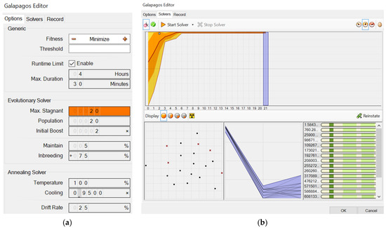
Figure 5.
The interface of the optimizing Galapagos application: (a) the initial values of internal configuration parameters, (b) the interface presenting the calculation results.
The top graph in Figure 5b shows the average fitness of the searched population for all genotypes (solutions). The observed upward trend and the variation in bandwidth in the subsequent generations indicate the effectiveness of the adopted algorithm. This graph shows convergence, i.e., the approach of the calculations to the optimal solution. The graph on the left is a series of points representing the subsequent best solutions throughout the optimizing process. The middle graph shows the efficiency of the calculations, i.e., the speed at which satisfactory results are obtained. The numbers on the right represent the current calculation accuracy.
To search for effective economic solutions, another twenty-two discrete output models Mfdeo,r (r from 21 to 42) were created based on the previously optimized models Mfdeo,r (r = 4, 7 and 13) and the functional dependencies defined by Equations (1)–(8). The specific property of these new Mfdeo,r models (r from 21 to 42) is that several different values of two independent variables Prc and Rcn were adopted, as shown in the third and the fourth columns of Table 5.
Table 5.
Characteristics of the new Mfdeo,r (r from 21 to 42) models describing various energy modernizing processes of a multi-story student residence hall.
The first column of Table 5 provides the designations of the new twenty-one models that are the result of twenty-one computational processes performed on the basis of the previous optimal simulation results. In the second column of Table 4, the designation of the basic optimal model is presented. The values of the Xi variables are taken from this basic model, except for the variables Prc and Rcn given in the third and the fourth columns.
The remaining columns of Table 5 provide a number of values of four dependent variables calculated for Mfdeo,r (r from 21 to 40), which differ from the values calculated previously for Mfdeo,r (r from 1 to 20). Thus, a number of calculations related to the changes in the prices Prc (presented in the third column) of energy supplied with an external grid and the changes in the ratio Rcn of the price of 1 m2 of PVI to the price of the energy supplied from the grid multiplied by 1000 were carried out using the Mfdeo,r (r from 21 to 40) models.
4. Analysis and Discussion
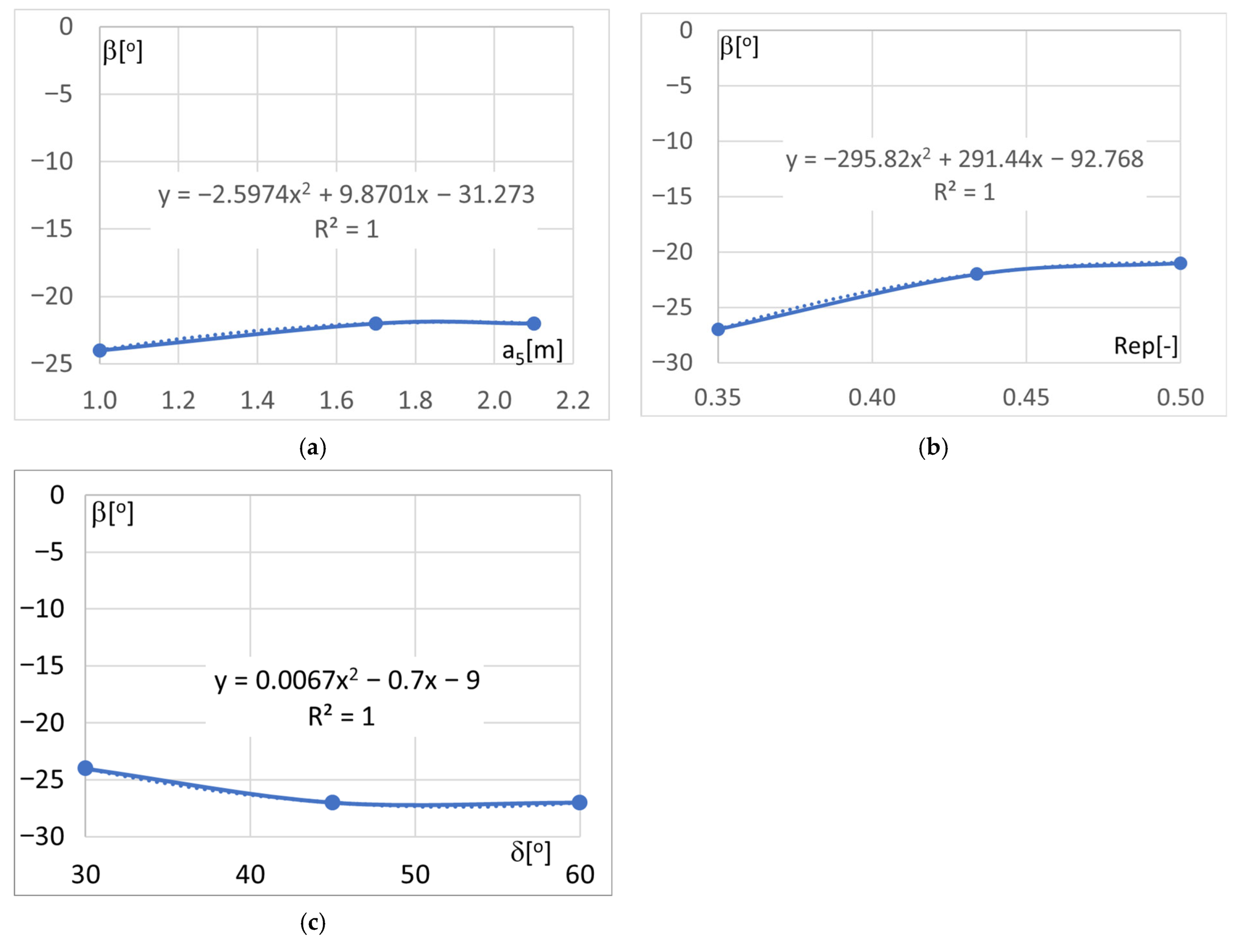
The characteristics of the discrete models Mfdeo,r (r from 1 to 20) presented in Table 4 result from the relationships established between the input parametric model Mfpg(Xi) and the output parametric model Mfpe(Yj) implemented in each optimizing process. The thick lines presented in the diagrams in Figure 6a–c represent non-linear relations between β (defining the optimal azimuth of the examined PVI) and (1) the height a5 of the PV panels employed, as shown in Figure 6a; (2) the Rep ratio, representing the replacement of energy delivered via the external grid with the electricity produced by the PV panels as shown in Figure 6b; (3) the angle δ defining the distances between subsequent rows of PVI panels, as shown in Figure 6c.
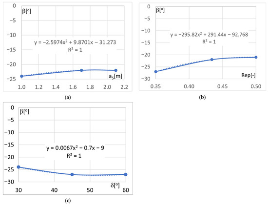
Figure 6.
Three diagrams presenting the relations between the optimized variable β and (a) a5, (b) Rep, and (c) δ found during the optimizing processes (the lines in blue).
The presented thick lines describe non-linear dependences between a5, δ, Rep, and the β optimal PVI’s azimuth. These dependences can be used to predict the expected values of β, γ, and Rat corresponding to the arbitrary values of a5, δ, and Rep different from the those presented in Table 3, Table 4 and Table 5. For these purposes, the thinner dashed regression lines are presented in these diagrams. Each figure also provides an equation corresponding to these regression lines. The considered lines and the ranges of a5, δ, and Rep indicate a significant influence of these variables on because their variation can lead to changes in the value of β up to 8%, 43%, and 12%, respectively, as shown in Figure 6a–c.
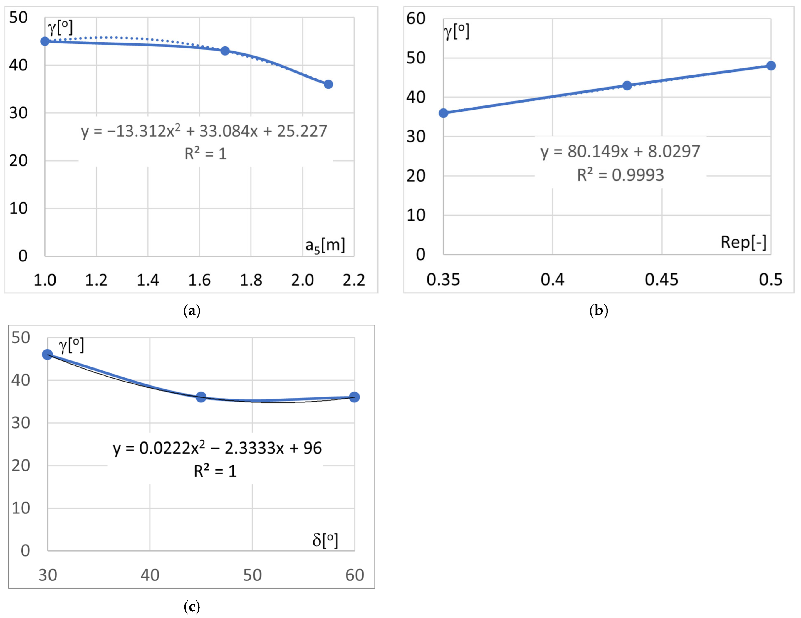
The diagrams shown in Figure 7a–c present the relationships between the optimal angles γ of inclination of the PV’s planes to the horizontal plane, and a5, δ and Rep. The presented lines indicate significant influences of these variables on variation of a5 causes significant changes in the value of γ up to 25%, as shown in Figure 7a. A change in Rep can also lead to a significant change in of γ up to 33%, as shown in Figure 7b. A change in δ can cause a less significant change in γ up to 12.5%, as shown in Figure 7c. The observed significant non-linear dependencies indicate the validity of using different inclinations of PV panels depending on their height, the quantity of the grid energy replacement rates, and the PV panel row spacing.
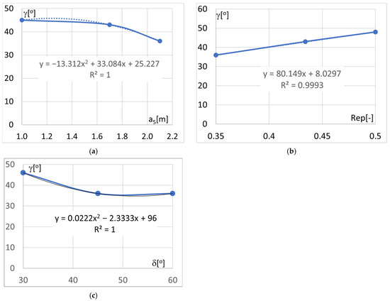
Figure 7.
Three diagrams presenting relations between γ and (a) a5, (b) Rep, and (c) δ found during the optimizing processes (the lines in blue).
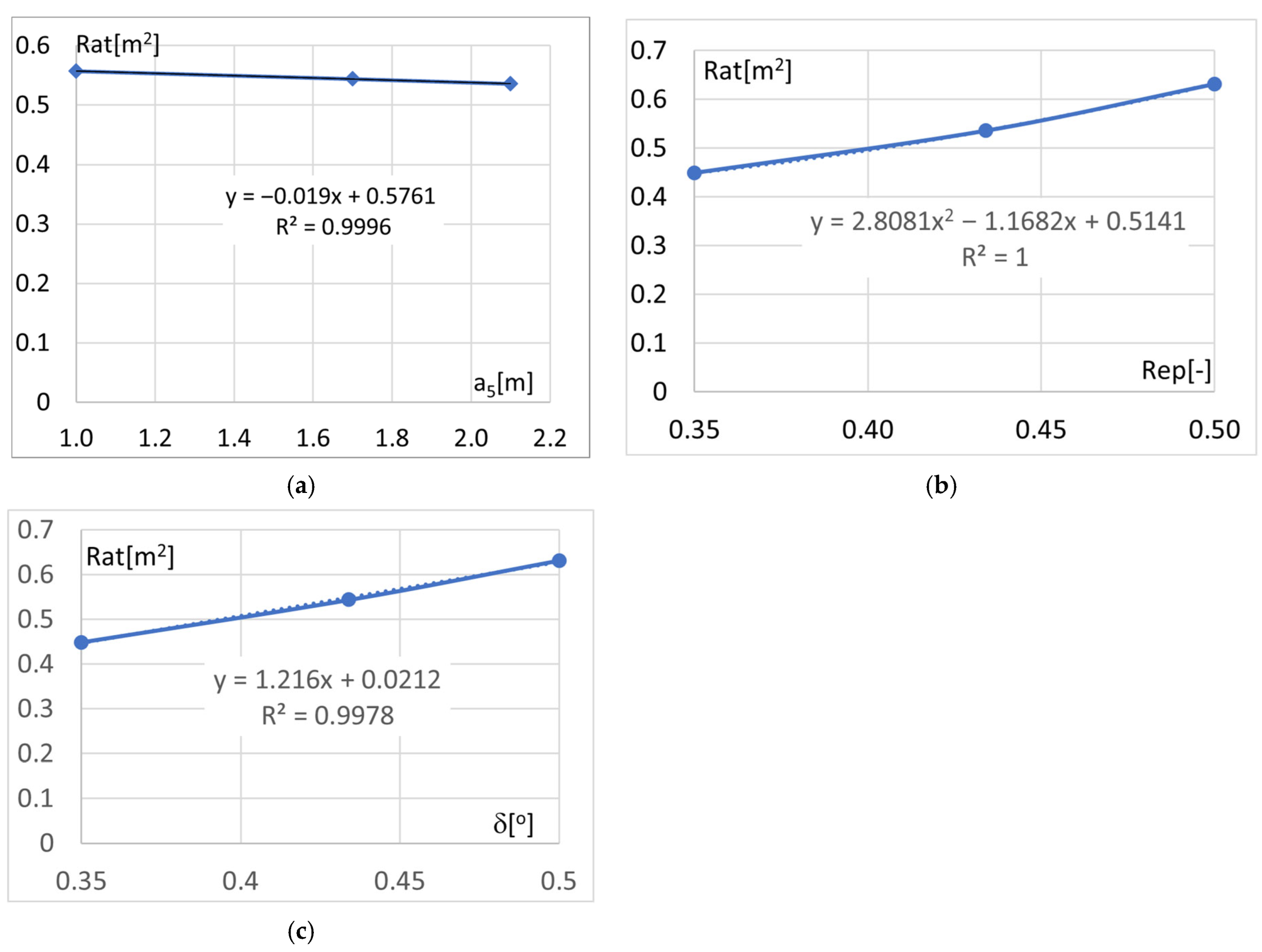
Figure 8a–c shows three nearly straight thick lines presenting the relations between Rat (the ratio of surface area of all PV panels to roof surface area) and a5, δ, and Rep. The influence of a5 on Rat is insignificant, as shown in Figure 8a. The relationship between Rat and Rep is significant and slightly non-linear, as shown in Figure 8b. A variation in Rep can cause a change in Rat of up to 40%. A significant change in the value of Rat up to 40% can be caused by a variation in δ, as shown in Figure 8c.
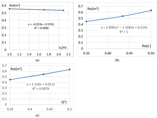
Figure 8.
Three diagrams presenting relations between Rat and (a) a5, (b) Rep, and (c) δ found during the optimizing processes (the lines in blue).
All diagrams were made with the help of Excel [26]. They depict the relationships obtained as a result of the optimizing processes related to the geometry and orientation of the PV panels. In turn, the relationships obtained in the second step presented below concern economic aspects of the dormitory renovations. The important arbitrary investment efficiency indicators are the PBK payback period, the CTS total PVI costs, and the RER annual profits resulting from replacing the various parts of the grid energy with electricity produced by the PVI. The performed calculations do not take into account inflation and investment interest. In addition, the variations in the grid energy prices and PVI costs were assumed to be uniform.
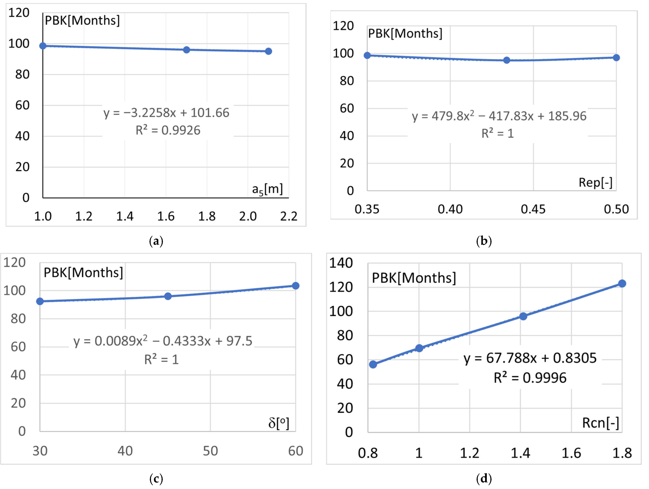
Figure 9a,b shows a negligible impact of a5 and Rep on the PBK payback period of investment in the PVI. The impact of a5 on PBK is insignificant (the observed changes are limited to 4%), as shown in Figure 9a. The relationship between PBK and Rep is almost linear, as shown in Figure 9b. A The possible changes in Rep can cause an insignificant variation in PBK up to 2%. However, changes in δ may cause significant changes in PBK up to 12%, as shown in Figure 9c. The optimized models Mfdeo,r (r from 1 to 20) created using constant values of Prc and Rcn made it possible to observe the relationships indicating that the payback period is almost unchanged. The impact became noticeable only in the cases where the distance between subsequent PVI rows was significantly reduced.
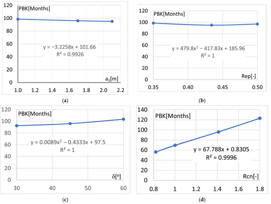
Figure 9.
Four diagrams presenting the relations between PBK and (a) a5, (b) Rep, (c) δ, and (d) Rcn found during the optimizing processes (the lines in blue).
Another relationship is shown in Figure 9d, where the thick line presents a strong linear relationship between the payback period PBK and the proportion Rcn of investment costs to the unit price of energy. The analyzed range of the changes in Rcn indicates large differences in the investment payback period. The relative values of these differences can reach up to 45%, which indicates a very significant impact of the grid energy prices on the PVI costs.
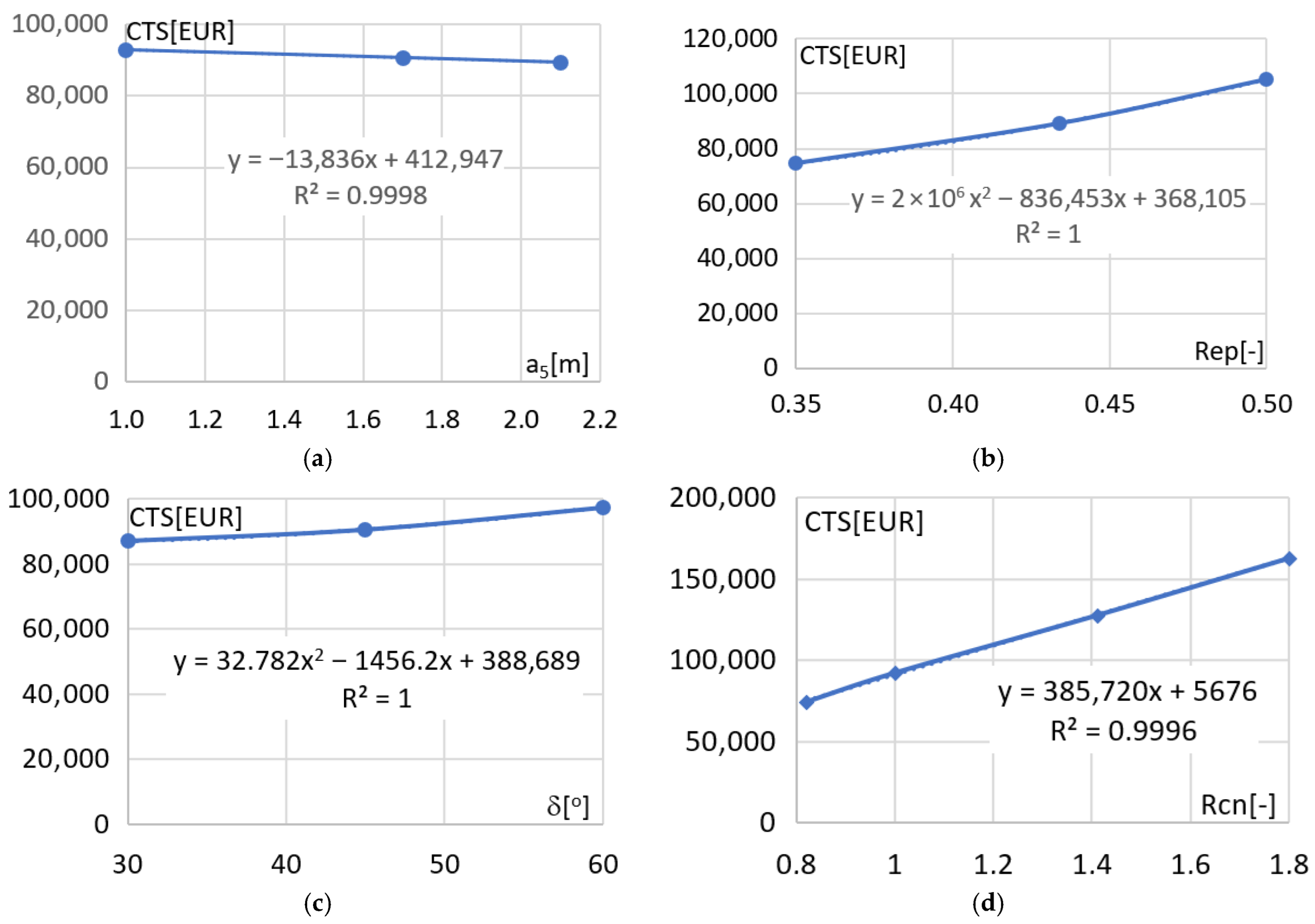
The lines presented in Figure 10a–d differ themselves noticeably in terms of their inclination and curvature. Figure 10a shows a negligible impact of a5 on the investment costs CTS, where any change in a5 causes an insignificant change in CTS (limited to 4%). In turn, Figure 10b shows a significant, linear impact of the Rep grid energy replacement rates on CTS. A change in Rep can cause a significant change in CTS up to 41%. The line presented in Figure 10c indicates a significant, linear relationship between CTS and the angle δ. A change in δ is able to cause a significant change in up to 12%.
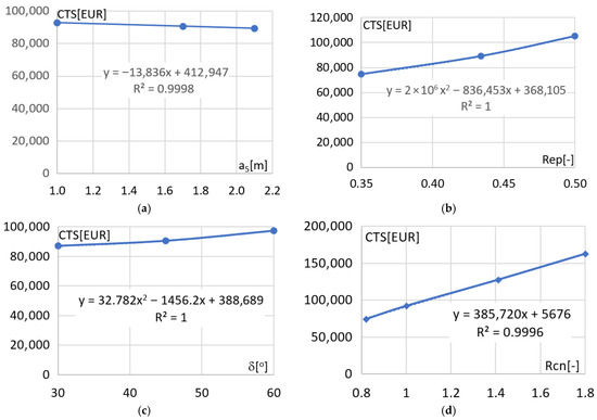
Figure 10.
The diagrams presenting relations between CTS and (a) a5, (b) Rep, (c) δ, and (d) Rcn found during the optimizing processes (the lines in blue).
The line shown in Figure 10d illustrates a very strong linear relationship between CTS and Rcn. The analyzed range of the possible changes in Rcn may result in very large variations in investment costs. The relative differences in CTS can reach 120%. This strong relationship indicates a significant impact of the unit costs of PVI on the total costs.
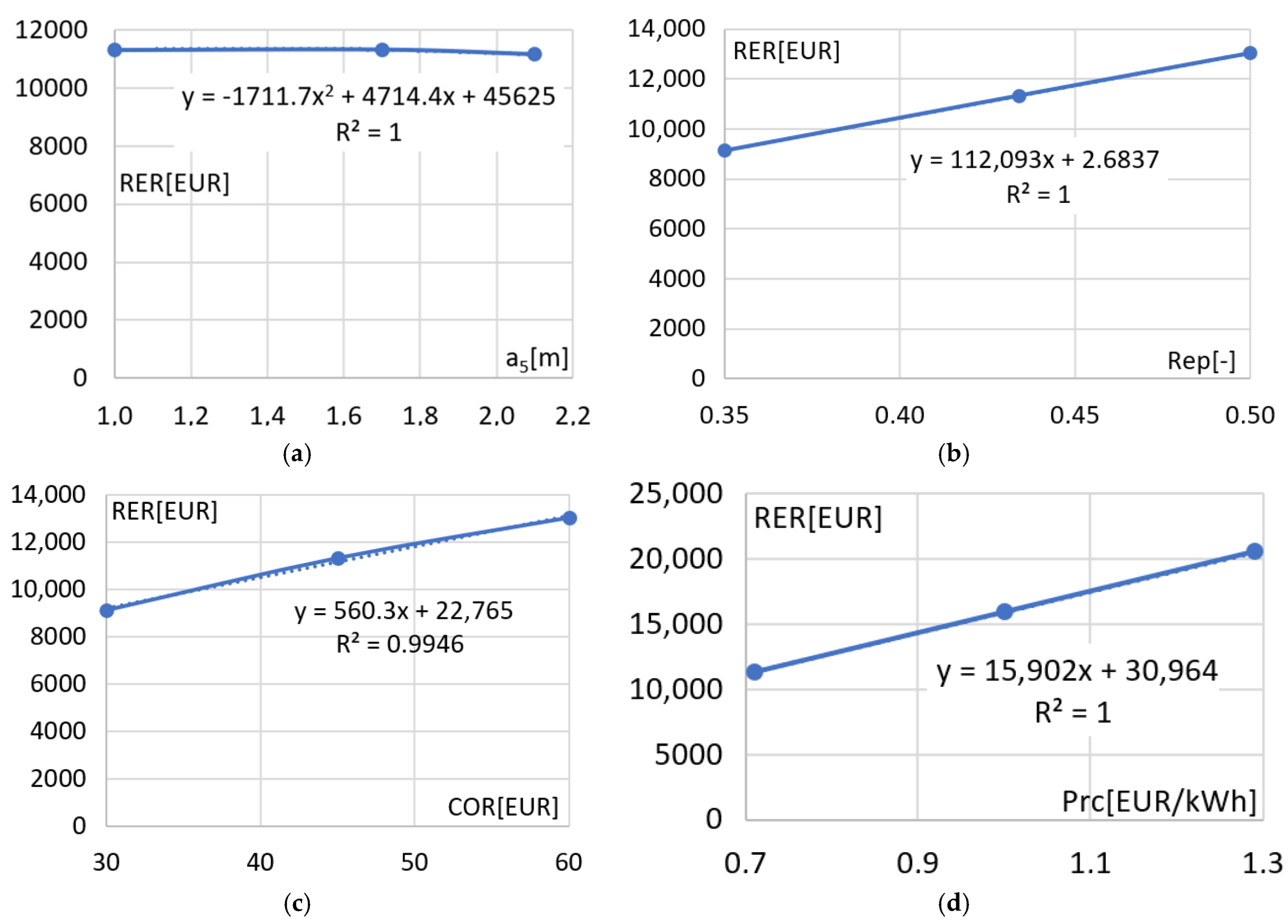
Four curves shown in Figure 11a–d present four relationships between the Prc annual price of the grid energy and the variables a5, δ, Rep, and Rcn. Figure 11a shows an insignificant impact of a5 on RER. The inclination of the line presented in Figure 11b shows a significant linear impact of Rep on RER. A change in δ can cause a significant variation in RER up to 41%. The line presented in Figure 11c indicates a significant linear relationship between RER and δ, where a variation in spacing of the subsequent PVI rows can cause significant changes in RER up to 43%.
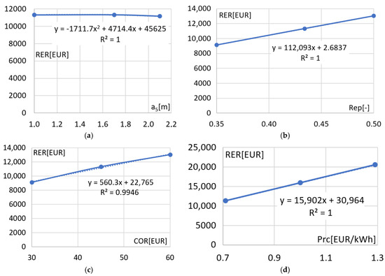
Figure 11.
Four diagrams presenting relations between Prc: (a) a5, (b) Rep, (c) δ, and (d) Prc found during the optimizing processes (the lines in blue).
The thick line in Figure 11d presents a very strong linear relationship between RER and Prc since the analyzed range of the possible changes in Prc indicates a variation in Prc up to 82%.
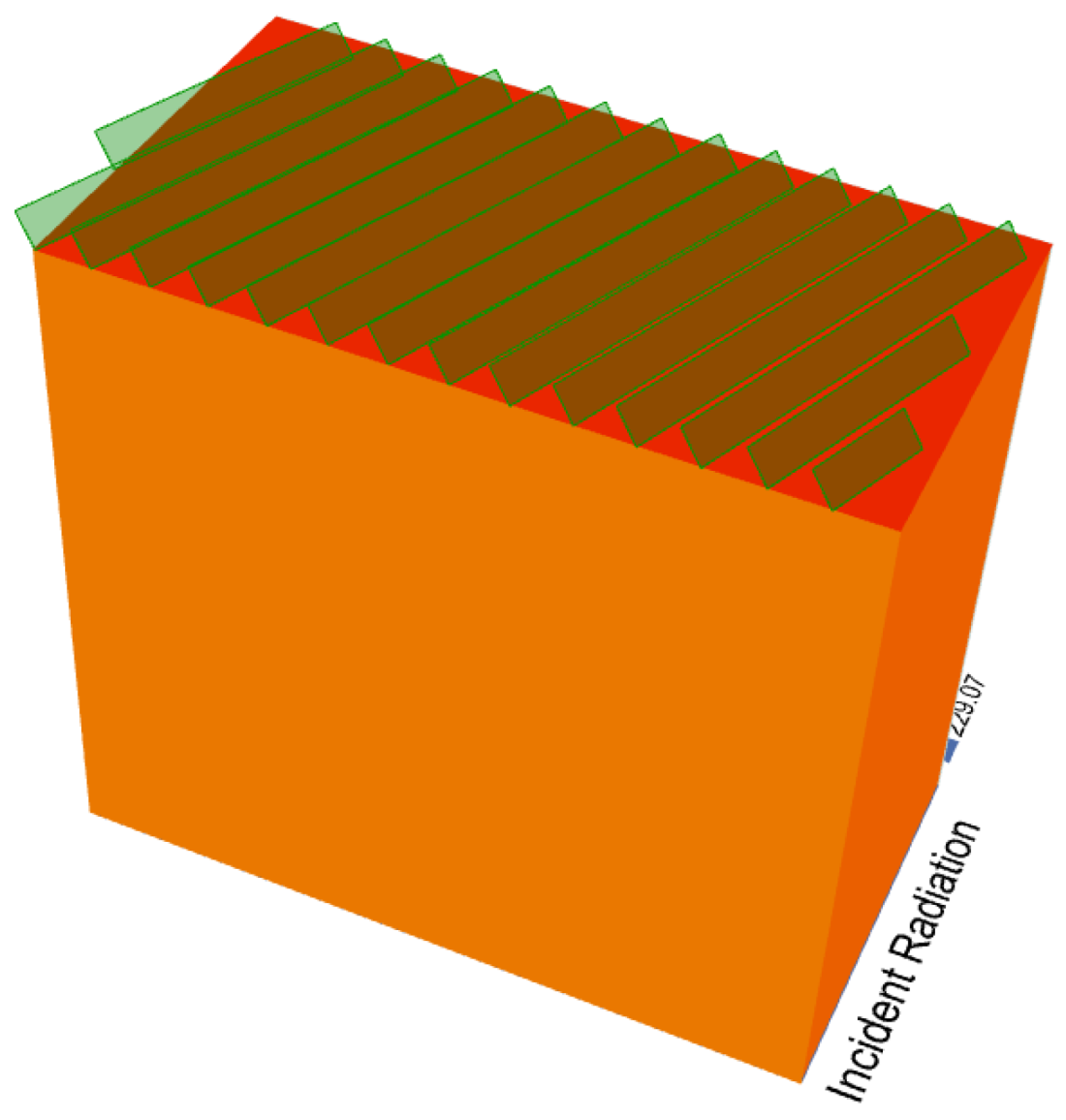
The Mdeo,7 model of the examined IKAR dormitory, developed using the novel application in Rhino/Grasshopper, is presented in Figure 12. This geometric model of a building and its PVI are used to simulate solar performance of its envelope and electricity production. The optimal model shown in Figure 12 enables the description of key observations that can subsequently be applied to other student residences. The figure illustrates a relatively steep inclination of the optimized PV panels to the horizontal plane and a high density of panel rows on the roof, and a significant difference between the azimuths of the PVI and the building façades. Such models facilitate the feasibility assessment of potential renovations for various existing buildings. The dark hues of the building façades and roof indicate the potential for effective utilization of the building envelope for PVI due to relatively high solar irradiance.
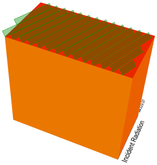
Figure 12.
A simplified model Mdeo,7 of the IKAR dormitory.
In addition, an analysis of the relationships presented in Figure 4, Figure 5 and Figure 6 leads to a fundamental conclusion that it is advisable to optimize all three variables: the β PV panel orientation, the γ PV panel tilt angle, and the Rat ratio of PVI area to roof area to achieve the energy efficiency of student dormitory renovations using PVI. In the examined ranges of variation in the a5 PV panel height, the δ angle determining the spacing of subsequent rows of PVI and the Rep grid energy replacement rates, it can be stated that Rep influences the optimized values of β, γ and Rat the most. Therefore, one should strive to obtain the highest possible value of Rep while maintaining the adopted boundary conditions. These relationships indicate that the individual geometric and physical characteristics of each dormitory under consideration should be optimized to effectively replace grid energy with electricity produced by the PVI.
Issues related to the Rep grid energy replacement rates were analyzed by H. Wu et al. [21], who considered this parameter within the range of 0.35 to 0.50 for cold regions of China. This range is similar to the boundary conditions used in the current article for an analogous moderate climate. In turn, A. Barman et al. [12] assumed a Rep value of 0.49 to be effective. These results are consistent with previous findings by Abramczyk and Bielak [2] regarding multi-story student dormitories, where PVIs were distributed on different facades and Rep was analyzed within the 0.434 to 1.0 range. Furthermore, A. Alqatamin and J. Su [20] showed that PVI can offset 0.15 to 0.87 of total grid load.
In the remaining instances, the influence of a5 and δ on the optimized values of β, γ, and Rat is significant; however, it is much smaller than in the case of Rep. An exception is the relationship between the optimized values of the variables δ and Rat, where the significant influence of the angle δ (defining the PV panel row spacing) on the roof area occupancy Rat. This implies a need to find an optimal value for δ that balances roof occupancy and inter-row shading resulting from maintenance and service constrains. These limitations necessitate the development of individual characteristics for each student dormitory under consideration, preferably during the building design step.
Geometrically optimized models were further considered to determine the energy production and renovation costs. An analysis of the relationships presented in Figure 9c and Figure 10c, and Figure 11c show the significant impact of δ on the total cost CTS resulting from the 12% increase in CTS over the considered range of δ, as shown in Figure 9c. In the case of the PBK payback period, the increase amounted to 12% and was significant, as shown in Figure 10c. In the case of the annual profits RER resulting from replacing the grid energy, the increase was very significant and reached 43%, as shown in Figure 11c.
The presented approach to energy optimizing processes for dormitory renovations is an original achievement of the authors. It is based, among other factors, on the differences β between the building and PVI azimuths, and the angle δ defining the spacing between subsequent PVI rows. The obtained quantitative relationships are valid for buildings located in Central Europe in a temperate climate. The energy and estimated economic analyses facilitated the subsequent step of the optimizing processes, the results of which were compared with those of other researchers.
Based on the optimized values of β, γ, and Rat, and the boundary conditions for a5, δ, and Rcn, the analysis conducted using the diagrams in Figure 9 and Figure 10 showed that: 1. The impact of the a5 panel height on the retrofit efficiency CTS and PBK is very small, (Figure 9a and Figure 10a). 2. The impact of the δ angle (defining the distance between the PVI rows) on CTS and PBK is significant; however, in the case of RER, this impact is very significant (Figure 9b, Figure 10b and Figure 11b). 3. The impact of the Rep grid energy replacement rate on PBK is insignificant (Figure 9b), but it is very significant on β and Prc (Figure 10b and Figure 11b). 4. The impact of the ratio between PVI installation costs per 1 m2 of PVI and the grid energy price (of 1 kWh) on CTS and PBK is very significant (Figure 9d and Figure 10d). 5. The impact of the grid energy price on the profits resulting from replacing grid energy with electricity produced by the PVI is very significant (Figure 11d). Analogous dependencies occur regarding the influence of Rat on CTS, PBK, and RER.
Issues related to the PBK payback period were analyzed by A. Young-Sub et al. [16], who achieved an optimal payback period of nine years. L. Tao et al. [22] demonstrated that the energy generated by the PVI allows for an eight-and-a-half-year payback period. Abramczyk and Bielak [2] obtained a nine-year payback period for multi-story student dormitories where PVIs were placed on different facades. In the case of high variability in Rcn considered in the present article, the payback period ranges from six to ten years.
A. Alqatamin and J. Su [20] analyzed the parametric energy and economic characteristics of PVIs arranged on various roofs in different zones. They examined two types of buildings—villas and apartments—which offered 30% and 21% rooftop utilization for PVI, respectively. In the renovations under consideration, roof surface utilization was twice as high, ranging from 43% to 60%. These results suggest that in future analyses, the roof surface utilization may achieve significantly higher values than previously recorded, necessitating the design of an appropriate area of each roof slope.
5. Conclusions
The presented novel method for renovating multi-story student dormitories with photovoltaic installations was based on iterative computer simulations that lead automatically to optimal results in the dormitory renovation processes. The first step of the algorithm focuses on the geometric characteristics of the PVI. In the second step, based on the obtained optimal geometric features, energy and cost optimizations were performed, taking into account the payback time for the modernization costs. Ultimately, a single discrete model was selected from forty-two optimal models that satisfied the optimizing conditions of both the first and second steps of the algorithm. All discrete models were constructed using previously defined, innovative parametric models of PVIs integrated into dormitory roofs.
The single example discrete model was presented in detail, characterized by the following specific optimized values of several selected parameters. The difference between the building’s and the PVI’s azimuths is −21°. The PV panel tilt angle to the roof plane is 48°. The ratio of the PV panel surface area to roof surface area is 0.632 (dimensionless). The angle defining the spacing between subsequent PV panel rows is 45°. For this geometric configuration, the optimal payback period was calculated as 97 months, with an annual return of EUR 16,478.20 and a total renovation cost of EUR 133,106. For all optimized PVI configurations, the optimal PBK payback period was ranged from 92 to 103.5 months assuming the boundary condition that network energy prices and PVI installation costs are proportionally changed. If the Prc grid energy price and the Rcn PVI costs vary disproportionately, the PBK payback period can range from 56 to 126 months.
It is intended that the obtained results will be compared and combined with those derived from the renovation of multi-story student dormitory façades. These activities aim to develop a comprehensive method for the renovation of student dormitories, supporting their systematic design and optimization.
Author Contributions
Conceptualization, J.A.; methodology, J.A.; software, J.A. and W.B.; validation, J.A. and W.B.; formal analysis, J.A. and W.B.; investigation, J.A.; resources, J.A. and W.B.; data curation, J.A. and W.B.; writing—original draft preparation, J.A.; writing—review and editing, J.A. and W.B.; visualization, J.A. and W.B.; supervision, J.A.; project administration, J.A.; funding acquisition, J.A. All authors have read and agreed to the published version of the manuscript.
Funding
Financial support was obtained from the Department of Architectural Design and Engineering Graphics of the Rzeszow University of Technology and the Discipline Council of Civil Engineering, Geodesy and Transport at Rzeszow University of Technology.
Data Availability Statement
The original contributions presented in this study are included in the article. Further inquiries can be directed to the corresponding authors.
Acknowledgments
We would like to thank the Head of the Department of Architectural design and Engineering Graphics for financial support and the Head of the discipline of Civil Engineering, Geodesy and Transport.
Conflicts of Interest
The authors declare no conflicts of interest. The funders had no role in the design of the study; in the collection, analyses, or interpretation of data; in the writing of the manuscript, or in the decision to publish the results.
Abbreviations
The following abbreviations are used in this manuscript:
| Photovoltaic installation | |
| Photovoltaics | |
| Independent i-th variable | |
| Dependent j-th variable | |
| Mfpg | Qualitative parametric input model |
| Mfdg,k | Quantitative discrete k-th input model |
| Mfdeo | Qualitative parametric output model |
| Mfdeo,r | Quantitative discrete r-th output model |
| Mfpe | Quantitative parametric output energy model |
| Etot | Energy supplied from a grid |
| dEtot | Accuracy of calculations related to the energy produced by PV |
| δ | Angle defining the spaces between the subsequent rows of PV panels |
| γ | Angle of the tilt of PV panels |
| α | Azimuth of building |
| β | Angle of difference between the azimuth of PV panels and the azimuth of building |
| a5 | Height of each PV panel |
| Rat | Ratio of the surface area of all PV planes to the surface area of roof |
| Rep | Net energy replacement rates related to replacement of the net energy by electricity produced by PVI |
| Prc | Price of the 1 kWh net energy |
| Rcn | Ratio of the renovation costs to the net energy prices multiplied by 1000 |
| CTS | Costs of PVI |
| PBK | Payback period of the renovating investment |
| TSP | Total surface area of the panels distributed on a roof |
| AOP | Roof area occupied by the PV panels |
| COR | Total cost of constructing 1 m2 of PVI |
| AEL | Amount of electricity produced by PVI |
| RER | Net energy replacement rates defining the cost of the net energy replaced by electricity produced by PV panels during the year |
References
- Neteler, M.; Mitasowa, H. Open Source GIS a Grass Gis Approach, 3rd ed.; Springer: New York, NY, USA, 2008. [Google Scholar]
- Abramczyk, J.; Bielak, W. An Automated Method for Optimizing the Energy Efficiency of Multi-Story Student Residence Halls Using Façade Photovoltaic Installations. Energies 2025, 18, 5637. [Google Scholar] [CrossRef]
- Chwieduk, D. Solar Energy in Buildings, 1st ed.; Science Direct; Academic Press: London, UK; Elsevier Science & Technology: London, UK, 2014. [Google Scholar] [CrossRef]
- Liu, J.; Zang, H.; Zhang, F.; Cheng, L.; Ding, T.; Wei, Z.; Sun, G. A hybrid meteorological data simulation framework based on time-series generative adversarial network for global daily solar radiation estimation. Renew. Energy 2023, 219, 119374. [Google Scholar] [CrossRef]
- Súri, M.; Dunlop, E.D.; Jones, A.R. GIS-based inventory of the potential photovoltaic output in Central and Eastern Europe. In Proceedings of the Photovoltaic in Europe: From PV Technology to Energy Solutions Conference and Exhibition, Rome, Italy, 7–11 October 2002. [Google Scholar]
- Buchalova, D.; Hofierka, J.; Supinsky, J.; Kanuk, J. Estimating Subcanopy Solar Radiation Using Point Clouds and GIS-Based Solar Radiation Models. Remote Sens. 2025, 17, 328. [Google Scholar] [CrossRef]
- Mueller, R.; Matsoukas, C.; Gratzki, A.; Behr, H.; Hollmann, R. The CM-SAF operational scheme for the satellite based retrieval of solar surface irradiance—A LUT based eigenvector hybrid approach. Remote Sens. Environ. 2009, 113, 1012–1024. [Google Scholar] [CrossRef]
- European Commission Science Hub PVGIS. Available online: https://ec.europa.eu/jrc/en/PVGIS/docs/methods (accessed on 10 May 2025).
- Kabir, H.; Abu Jihad, H.; Chowdhury, S. Analysis of Solar Panel Power Investigation using Fixed Axis, Single Axis and Dual Axis Solar Tracker. 4th International Conference on Evolutionary Computing and Mobile Sustainable Networks. Procedia Comput. Sci. 2025, 252, 708–714. [Google Scholar] [CrossRef]
- Qadeer, A.; Parvez, M.; Khan, O.; Jafri, H.Z.; Lal, S. Optimization of solar radiation on tilted surface in isotropic and anisotropic atmospheric conditions. Next Res. 2024, 1, 100075. [Google Scholar] [CrossRef]
- Poornima, P.U.; Dhineshkumar, K.; Kumar, C.K.; Sumana, S.; Rama Sundari, M.V.; Sivaraman, P.; Shuaib, M.; Rajaram, A. Optimising rooftop photovoltaic adoption in urban landscapes: A system dynamics approach for sustainable energy transitions. Biomed. Signal Process. Control 2025, 100, 107071. [Google Scholar] [CrossRef]
- Barman, A.; Muiz, M.; Sharif, A. Performance Analysis of Building Integrated Photovoltaic of High-Rise Buildings in Urban Areas, Oumma Marium Mishu, Mohammed Belal Hossain Bhuiyan, Mohaimenul Islam, December 2021. In Proceedings of the 2021 IEEE PES Innovative Smart Grid Technologies—Asia (ISGT Asia), Brisbane, Australia, 5–8 December 2021. [Google Scholar] [CrossRef]
- Kaitouni, S.I.; Gargab, F.Z.; Es-sakali, N.; Mghazli, M.O.; Mansouri, F.; Jamil, A.; Ahachad, M. Digital workflow for nearly zero-energy high-rise office building design optimization at the district scale in Mediterranean context. Energy Built. Environ. 2024; in press. [Google Scholar] [CrossRef]
- Abramczyk, J.; Bielak, W. Parametric Building Envelopes Rationalized in Terms of Their Solar Performance in a Temperate Climate. Energies 2025, 18, 2479. [Google Scholar] [CrossRef]
- Aste, N.; Del Pero, C.; Leonforte, F.; Ounis, S.; Abdelrahim, A.M.G. The role of photovoltaic technology in achieving net zero energy target in residential buildings. Energy Strategy Rev. 2024, 55, 101543. [Google Scholar] [CrossRef]
- Young-Sub, A.; Jongkyu, K.; Hong-Jin, J.; Gwang-woo, H.; Haneul, K.; Wangje, L.; Min-Hwi, K. Retrofit of renewable energy systems in existing community for positive energy community. Energy Rep. 2023, 9, 3733–3744. [Google Scholar] [CrossRef]
- Kazemian, A.; Xiang, C. Synergizing photovoltaic-thermal systems with green roofs: A pathway to enhanced urban sustainability and energy efficiency. Renew. Sustain. Energy Rev. 2025, 222, 116002. [Google Scholar] [CrossRef]
- Paphapote, T.; Bamrungsawat, W.; Wongwuttanasatian, T. Inclination and inter-row spacing optimization for 12MW floating photovoltaic system with shading loss and financial analysis. Results Eng. 2025, 27, 106362. [Google Scholar] [CrossRef]
- Shekar, V.; Abraham, D.; Caló, A.; Pongráacz, E. Determining the optimal azimuth for solar-ready buildings: Simulating for maximising the economic value of solar PV installations in Lapland Finland. Renew. Energy 2025, 241, 122357. [Google Scholar] [CrossRef]
- Alqatamin, A.; Su, J. Machine learning prediction of photovoltaic-thermal system with V-shaped perforated fins. Appl. Therm. Eng. 2025, 280, 128344. [Google Scholar] [CrossRef]
- Wu, H.; Deng, F.; Tan, H. Research on parametric design method of solar photovoltaic utilization potential of nearly zero-energy high-rise residential building based on genetic algorithm. J. Clean. Prod. 2022, 368, 133169. [Google Scholar] [CrossRef]
- Tao, L.; Wang, M.; Xiang, C. Assessing urban morphology’s impact on solar potential of high-rise facades in Hong Kong using machine learning: An application for FIPV optimization. Sustain. Cities Soc. 2024, 117, 105978. [Google Scholar] [CrossRef]
- Movahhed, Y.; Safari, A.; Motamedi, S.; Khoshkhoo, R.H. Simultaneous use of PV system and green roof: A techno-economic study on power generation and energy consumption. Energy Procedia 2019, 159, 478–483. [Google Scholar] [CrossRef]
- Maurer, B.; Lienert, J.; Cook, L. Comparing PV-green and PV-cool roofs to diverse rooftop options using decisions analysis. Build. Environ. 2023, 245, 110922. [Google Scholar] [CrossRef]
- Rhinoceros. Rhino. Available online: https://www.rhino3d.com/ (accessed on 10 May 2025).
- Office. Excel. Available online: https://chromewebstore.google.com/ (accessed on 10 May 2025).

Disclaimer/Publisher’s Note: The statements, opinions and data contained in all publications are solely those of the individual author(s) and contributor(s) and not of MDPI and/or the editor(s). MDPI and/or the editor(s) disclaim responsibility for any injury to people or property resulting from any ideas, methods, instructions or products referred to in the content. |
© 2026 by the authors. Licensee MDPI, Basel, Switzerland. This article is an open access article distributed under the terms and conditions of the Creative Commons Attribution (CC BY) license.