Research on Deformation Fault Diagnosis of Transformer Windings Based on a Highly Sensitive Multimodal Feature System

Abstract

The current mainstream methods for online detection of transformers all have shortcomings such as low sensitivity and susceptibility to interference from the testing environment. Aiming at the shortcomings of the existing online detection methods for transformer winding deformation in terms of feature sensitivity and diagnostic accuracy, this paper proposes a fault intelligent diagnosis method based on high sensitivity multimodal feature fusion. First, the winding deformation experiment is designed for typical fault data, which is obtained to extract multiple frequency and time domain response features and construct a multidimensional feature library. Subsequently, principal component analysis is used to evaluate the sensitivity of each feature to different faults and establish a highly sensitive multimodal feature system. On this basis, a TCN-BiGRU-PHA diagnostic model combining time convolutional network, bidirectional gated loop unit and attention mechanism is constructed to realize accurate identification of winding deformation faults. The experimental results show that the method has higher recognition accuracy under multiple types of faults, which provides feasible ideas and methodological support for realizing online intelligent monitoring of transformer winding deformation.

1. Introduction

As critical equipment in power transmission and distribution systems, the operational status of power transformers directly impacts grid safety and power supply stability. Due to prolonged exposure to electrodynamic forces, thermal stresses, and short-circuit impacts, transformer windings are highly susceptible to structural deformation failures such as axial displacement, radial expansion, and interturn short circuits. These structural changes can cause localized electric field distortion and insulation degradation, potentially leading to internal discharges or breakdowns in severe cases. Relevant statistical data indicates that over 50% of major transformer failures are closely related to mechanical deformation of the windings [1,2]. Therefore, developing efficient and reliable detection technologies for winding deformation holds significant theoretical value and engineering importance.

Regarding the online detection of transformer windings, extensive research has been conducted in both academic and engineering circles, resulting in the development of various fault detection methods such as the short-circuit impedance method, vibration analysis, frequency response analysis (FRA), and voltage-current trajectory analysis (ΔU-I trajectory method) [3,4,5]. Among these, frequency response analysis is highly recommended by the IEEE C57.149 standard [6] and CIGRE technical documents as a key method for diagnosing mechanical faults in transformer windings due to its exceptional sensitivity to structural changes in the frequency domain. By comparing the amplitude-frequency or phase-frequency response curves of transformers under different operating conditions, FRA can effectively identify localized changes or overall displacement in transformer winding structures. It has been widely applied in field offline testing and condition assessment.

However, traditional FRA methods suffer from two core issues: first, they rely on complex excitation and frequency-sweeping systems, making true online testing difficult to achieve; second, measurement results are highly sensitive to boundary conditions such as external wiring configurations, load states, and power supply fluctuations, resulting in poor test repeatability and comparability [7]. To overcome these limitations, the impulse frequency response method (IFRA) based on short-pulse excitation has gained prominence in recent years. This approach replaces continuous sweep signals with short broadband pulses, enhancing response speed and online adaptability while maintaining spectral coverage. It demonstrates strong potential for field deployment [8,9,10,11,12].

Meanwhile, another time-domain response-based analysis method—the ΔU-I trajectory method—demonstrates high recognition capability in detecting transformer winding deformation. This method measures the time-series signals of excitation voltage and response current, plotting voltage-current trajectory curves at specific frequencies to visually reflect the structural mismatch characteristics of windings caused by changes in electrical parameters [13]. Research indicates that the ΔU-I trajectory method offers good feature discrimination in identifying typical deformation conditions such as interturn short circuits and winding displacement, while exhibiting strong interference resistance, particularly suitable for low-frequency detection [14]. Furthermore, compared to frequency-domain methods, the ΔU-I method is less dependent on testing equipment and wiring configurations, thereby enhancing repeatability and stability to a certain extent.

Although both IFRA and ΔU-I trajectory methods possess distinct advantages, current research predominantly focuses on validating the detection capabilities of individual methods across different fault modes. Systematic studies integrating both approaches to establish a multidimensional fault feature system remain scarce. And the fact that the equivalent network parameters of the FRA method are affected by the test environment and the ΔU-I is limited by the strong coupling characteristics of the voltage and current signals, this method has a feature confusion phenomenon in the scenario of concurrent multiple faults. Existing literature, such as Vahid Behjat et al. [15], employs frequency response curves to extract frequency-domain features for machine learning classification, achieving significantly improved accuracy. A. Abu-Siada et al. [16] attempted to feed ΔU-I trajectory images into convolutional neural networks for recognition, preliminarily validating the method’s feasibility in fault mode discrimination. However, these studies have yet to overcome the limitations of “information silo” analysis, failing to fully exploit the complementarity between the two methods across dimensions such as frequency-domain versus time-domain, low-frequency versus high-frequency, and morphological versus spectral features [17,18]. In response to the technical bottlenecks of traditional intelligent diagnosis algorithms, deep learning models have been innovatively applied in the field of power equipment condition monitoring [19]. Vatsa A et al. [20] utilized the Convolutional Neural Network (CNN) to identify the image or signal features related to transformer faults. Different algorithms have their own advantages when dealing with different types of data. By integrating them, complementary advantages can be achieved, which not only enhances the feature extraction ability of the model but also improves the prediction accuracy of the model [21,22,23].

Against the backdrop of increasingly complex and large-scale transformer structures, the limitations of single-feature extraction pathways in terms of sensitivity, stability, and adaptability have become increasingly apparent. Particularly in field environments characterized by complexity and strong nonlinear fault evolution, relying solely on a single method can easily lead to misdiagnosis or missed detection. Consequently, a growing number of researchers are focusing on the application of multi-source signal fusion analysis and collaborative feature extraction techniques in power equipment diagnostics [24,25].

Based on this, this paper proposes a detection approach that integrates IFRA analysis with the ΔU-I trajectory method, aiming to establish a feature system capable of both high-frequency response and low-frequency structural sensitivity. Regarding the integration strategy, this paper extracts full-frequency distribution characteristics from the IFRA curve and morphological geometric parameters from the ΔU-I trajectory diagram. Principal Component Analysis (PCA) is employed to reduce the dimensionality of high-dimensional features, establishing an integrated feature indicator system to enhance the discrimination capability of fault identification.

This fusion strategy offers the following advantages:

• It addresses the insufficient sensitivity of IFRA frequency domain responses in the low-frequency range;
• It enhances the modeling capability and interpretability of the ΔU-I trajectory method in the mid-to-high frequency range;
• Through multi-source feature fusion, it improves the detection system’s adaptability to different operating conditions and fault types;
• Combined with PCA, it further strengthens feature selection, enhancing algorithm stability and computational efficiency.

In summary, this paper innovatively proposes a transformer winding fault detection method based on IFRA and ΔU-I trajectory feature fusion. By integrating time-frequency domain signal processing and statistical feature analysis, it offers a novel approach for achieving online condition awareness of transformer windings and lays the foundation for fault type identification and predictive maintenance.

2. Principles of Online Detection Methods for Winding Deformation

2.1. Principles of Pulse Frequency Response Analysis

The pulse frequency response method is developed based on the fundamental principles of the frequency response method. Its key principle can be summarized as follows: a nanosecond pulse signal is applied to the transformer winding, and the response signal of the winding is then measured. By analyzing and processing this signal, the response characteristics of the winding at different frequencies can be obtained. The transformer winding can be modeled as a passive two-port network, whose circuit schematic is shown in Figure 1:

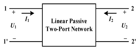
Figure 1. Transformer two-port network equivalent circuit model.

In this equivalent circuit, when an excitation voltage signal $u(t)$ is applied, the differential equation of the circuit derived from Kirchhoff’s laws is given by Equation (1).

$$u(t)=R_i(t)+L{\displaystyle \frac{di(t)}{dt}}+{\displaystyle \frac{1}{C}}{\displaystyle {\int }_0^{t}i\left(\tau \right)}d\tau$$

(1)

Among them, u(t) represents the applied excitation voltage signal, i(t) is the winding response current, R is the equivalent resistance, L is the equivalent inductance, and C represents the equivalent capacitance.

The pulse frequency response method employs nanosecond pulses as excitation signals. The time-domain expression of the nanosecond pulse signal $u_p(t)$ can be determined based on the specific pulse type. For instance, the expression for a common rectangular pulse is shown in Equation (2),

$$u_p(t)=\left\{\begin{array}{l}A,0\le t\le T_P\\ 0,t>T_P\end{array}\right.$$

(2)

where A represents the pulse amplitude and $T_p$ denotes the nanosecond pulse width. Applying this nanosecond pulse signal to the input terminal of the transformer winding equivalent circuit, the output response current $i_p(t)$ can be obtained by convolving the input pulse signal $u_p(t)$ with the circuit response $h(t)$ according to the convolution theorem, as shown in Equation (3).

$$i_p(t)=u_p(t)·h(t)={\displaystyle {\int }_{-\infty }^{+\infty }{u}_p(\tau )}h(t-\tau )d\tau$$

(3)

By measuring excitation and response signals, the response characteristics of windings at different frequencies can be calculated. Comparing the calculated frequency response curves with those under normal conditions enables the detection of faults such as winding deformation. When deformation occurs, it alters parameters like inductance and capacitance in the equivalent circuit of the winding, thereby changing the frequency response curve—manifesting as shifts in resonance frequency or variations in amplitude.

2.2. Principles and Standardization Methods of the ΔU-I Trajectory Approach

The ΔU-I trajectory method monitors voltage changes and corresponding currents on both the primary and secondary sides of transformer windings in real time. It plots trajectory characteristic curves for both sides under different operating conditions, then evaluates winding status based on the curve profiles. In the T-equivalent circuit of a single-phase transformer, terminal voltage and current can be expressed as sine functions, as shown in Equation (4).

$$\left\{\begin{array}{l}u(t)=U\cos (wt+{\phi }_1)\\ i(t)=I\cos (wt+{\phi }_2)\end{array}\right.$$

(4)

In the equation: u(t) and i(t) represent the terminal voltage and current of the transformer, respectively; U and I denote the voltage amplitude and current amplitude, respectively; φ₁ and φ₂ denote the initial phase angles of the voltage and current, respectively; ω is the angular frequency; t is time. Eliminating the common parameter t from Equation (4) yields the composite parametric equation shown in Equation (5).

$${\displaystyle \frac{i^2}{I^2}}+{\displaystyle \frac{u^2}{U^2}}-{\displaystyle \frac{2ui}{UI}}\cos ({\phi }_2-{\phi }_1)={\sin }^2({\phi }_2-{\phi }_1)$$

(5)

When φ₂ − φ₁ takes different values, the graphical representation of this parametric equation in the Cartesian coordinate system also varies. Under most operating conditions, a certain phase shift typically exists between the voltage and current of power transformers. Consequently, the trajectory curves constructed from voltage and current signals often exhibit elliptical distributions. When deformation faults occur in transformer windings, the corresponding ΔU-I trajectory curves also change. By monitoring and analyzing these trajectory variations, potential winding faults in transformers and their specific types can be effectively identified.

3. Winding Deformation Fault Testing and Sample Data Acquisition

3.1. Transformer Winding Deformation Fault Test

3.1.1. Introduction to the Transformer Experiment Simulation Platform

The joint analysis method proposed in this paper is primarily applied to large power transformers. Using actual large transformers as experimental subjects directly presents numerous challenges, such as their massive size, high cost, complex structure, and difficulty in replacement. In light of these issues, our research team collaborated with a transformer manufacturer to develop a model transformer specifically designed for winding deformation experiments, as shown in Figure 2a. This experimental transformer has a rated withstand voltage of 10 kV. However, its internal insulation structure and support components were designed and manufactured at a scaled-down proportion based on a 110 kV three-phase power transformer. This approach ensures experimental controllability while preserving typical structural characteristics. Detailed technical parameters are listed in Table 1.

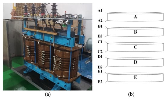
Figure 2. Schematic diagram of analog test transformer and middle replaceable winding. (a) Test transformer (b) Center-tap replaceable winding.

Table 1. Basic parameters of transformer construction.

Parameters	Rated Value
Rated Voltage (kV)	10/0.4
Capacity (kVA)	400
Rated Current (A)	23/577
Frequency (Hz)	50
Number of Phases	3
Connection Group	Ynyn0

The transformer used in this experiment features a specially designed high-voltage winding structure. The central section comprises ten sequential windings divided into five sets of dual-disc winding units that can be individually removed and replaced. This design enables flexible winding replacement, allowing different types of faulty windings to substitute for the original healthy windings during experiments to simulate various fault scenarios. Although the transformer employs an oil-immersed structure, the transformer oil itself becomes an interfering factor during winding fault setup and replacement operations. Therefore, the transformer oil must be drained and allowed to settle before proceeding with experimental operations.

To facilitate clear description and rapid localization of fault settings in subsequent experiments, a systematic numbering scheme was designed for the windings in the central structure. During the experiment, the five double-disc windings in the transformer’s central section were numbered sequentially from top to bottom as Groups A through E, with each group comprising two disc-shaped windings. Similarly, each of the five coils corresponding to a winding is equipped with two lead-out terminals. To ensure accurate identification of different winding positions during detection and data acquisition, all lead-out terminals were also numbered sequentially from top to bottom as A1, A2, …, E2, as shown in Figure 2b.

The main circuit for the transformer winding deformation fault simulation test in this paper is shown in Figure 3, where the black line indicates that this platform supports online operation of the test transformer. Specifically, the power supply represents the 380 V three-phase AC power line connected to the grid, providing electricity for the entire experimental platform. Its connection is controlled by a circuit breaker, while the three-phase AC power is regulated by a voltage regulator capable of adjusting the output voltage from 0 to 700 V. Due to the high rated capacity of the test transformer, the experimental power supply cannot fully meet its power requirements. To achieve stable operation at rated current, a three-phase voltage regulator applies an effective voltage of approximately 100 V to the high-voltage side while maintaining the low-voltage side load current stable at 4 A. An IFRA-based winding detection device generates high-voltage nanosecond pulse signals, which are coupled to the transformer’s Phase A via a capacitive coupling sensor. The pulse signal has a pulse width of 400 ns and an amplitude of 2000 V. To ensure high-precision signal acquisition, this study employs a wide-band high-voltage probe and a wide-band current sensor to measure the excitation voltage signal at the same position on the transformer and the bushing response current signal at the neutral point, respectively. Simultaneously, a power frequency signal acquisition device measures the terminal voltage and current of the transformer. To reduce reactive power in the power supply, the total inductive load of the test transformer is compensated by a capacitor with a parallel capacitance of 250 μF.

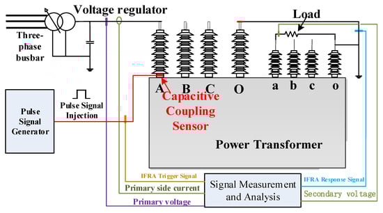
Figure 3. Transformer winding deformation fault simulation experiment wiring diagram.

This winding deformation simulation experiment selected the high-voltage side winding of Phase A as the test subject. The following testing plan was formulated to achieve the experimental objectives:

• To evaluate the repeatability of the testing method, a healthy winding was used as the test subject. Tests were conducted three times consecutively at one-week intervals.
• When simulating each type of winding deformation experiment, an interval of no less than 2 days was maintained, with a total of three tests conducted.
• Conduct baseline testing for background electromagnetic noise before and after experiments to eliminate environmental interference from experimental data, ensuring accurate reflection of winding conditions.
• When employing different online detection methods, maintain a minimum interval of 300 s between tests to prevent signal superposition interference from affecting results.

3.1.2. Winding Deformation Fault Simulation Experiment

(1)

Radial deformation

Transformer manufacturers additionally produce special radial deformation (RD) windings that can replace the middle ten winding cakes to simulate RD faults. These deformed windings feature radial deformation in multiple directions, with deformed sections offset by 90° from each other. The deformation level of the RD fault winding is characterized by the ratio of d to the radius r. The manufactured RD fault windings feature ratios of d to r at 3%, 5%, 7%, and 10%.

As observed in Figure 4a, the radial deformation of the winding exerts a relatively minor influence on the resonant peak and valley frequencies within the pulse frequency response, while significantly affecting the overall amplitude of the curve. Specifically, within the frequency range below 600 kHz, the positions of the resonance peaks and troughs remain largely stable. However, between 700 kHz and 1000 kHz, the resonance frequencies of the deformed windings exhibit a noticeable shift compared to the healthy state curve. Figure 4b displays the corresponding ΔU-I trajectory. Experimental data indicate that as the radial deformation rate of the winding gradually increases from 3% to 10%, its ΔU-I elliptical trajectory progressively diverges from the characteristic trajectory of the healthy state, exhibiting a trend of outward expansion.

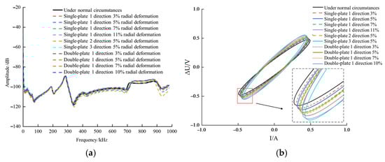
Figure 4. Frequency response curves under radial deformation faults. (a) Pulse Frequency Response Method (b) ΔU-I Trajectory Method.

(2)

Variation in Spacing Between Discs

Capacitance parameters play a dominant role in inter-disc spacing variation faults. Simulating faults can be achieved by connecting capacitors in parallel between two discs, while altering the capacitance value allows for modeling different degrees of faults. This paper simulates varying degrees of transformer winding faults by connecting capacitors with different parameter values in parallel between winding layers. Capacitance values include 100 pF, 200 pF, 400 pF, 600 pF, and 800 pF. The interlayer spacing variation fault is simulated according to the experimental setup shown in Table 2.

Table 2. Fault Setting Table.

Serial No.	Connector No.	Capacitance Value/pF	Serial No.	Connector No.	Capacitance Value/pF
1	A1-A2	50	5	A1-A2	800
2	A1-A2	67	6	C1-C2	400
3	A1-A2	100	7	E1-E2	400
4	A1-A2	200

Figure 5a shows the online pulse frequency response curve for faults involving variations in the spacing between laminations. In all fault scenarios, the parallel capacitance is positioned between joints A1 and A2. The figure reveals that such deformation faults primarily affect the online pulse frequency response characteristics above 250 kHz, manifesting as a frequency shift in the resonance peak.

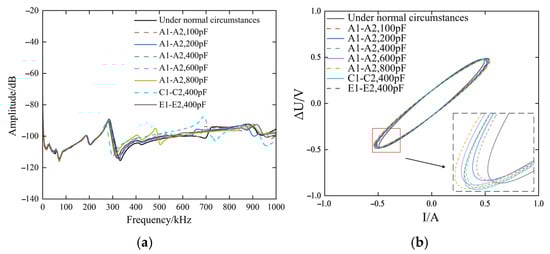
Figure 5. Frequency response curves under faults with varying inter-pie spacing. (a) Pulse Frequency Response Method (b) ΔU-I Trajectory Method.

Figure 5b shows the ΔU-I trajectory curve when a winding experiences a fault involving changes in the interlayer spacing. When such a fault occurs, the interlayer capacitance exhibits a nonlinear variation trend, causing both the major and minor axes of the ΔU-I trajectory to expand simultaneously. Compared to the characteristic changes induced by winding short-circuit faults, the trajectory alterations caused by inter-layer spacing variations are less pronounced. Thus, the sensitivity of the ΔU-I trajectory method is lower than that of the pulse frequency response method.

(3)

Axial deformation

Axial deformation faults are one of the common fault types in transformer windings, with relatively complex causes. To simulate axial deformation faults at different positions, the experiment employed a custom-made axial deformation winding to replicate this fault. There are two types of axial deformation: upward axial deformation (bulging deformation) and downward axial deformation (indentation deformation).

Figure 6a shows the online pulse frequency response curve during axial deformation faults. The curve exhibits amplitude shifts not only below 200 kHz but also above 300 kHz, with varying degrees of deviation. The figure also reveals that the nature of this amplitude deviation varies. When the winding exhibits upward axial deformation, the overall amplitude of its frequency response curve is higher than that of a healthy winding, indicating increased amplitude. Conversely, when the winding undergoes downward axial deformation, the overall amplitude of its frequency response curve is lower than that of the healthy curve. As the number of deformed winding layers increases—indicating greater deformation—the amplitude deviation becomes more pronounced.

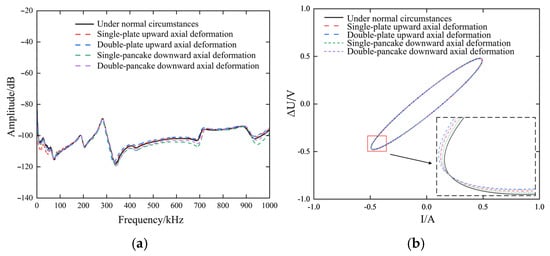
Figure 6. Frequency response curves under axial deformation faults. (a) Pulse Frequency Response Method (b) ΔU-I Trajectory Method.

As shown in the ΔU-I trajectory curve of Figure 6b, compared to radially deformed windings, axially deformed windings exhibit less pronounced changes in the ΔU-I trajectory characteristics, with smaller fluctuations in various characteristic parameters. The primary reason for this phenomenon lies in the limitations of manufacturing processes for deformed windings. Axial deformation achieves a relatively low displacement magnitude, and the distance between winding layers remains largely unchanged, making it difficult to simultaneously simulate axial misalignment across multiple winding layers. However, by analyzing the characteristic changes in the pulse frequency curve, the accuracy of fault diagnosis for axial deformation can be further enhanced.

3.2. Construction of a Highly Sensitive Multimodal Feature System Based on PCA

To investigate the matching degree between the equivalent circuit model constructed in this paper and the actual model, this section performs fault simulations on the established model based on winding fault experiments. It analyzes several common winding deformation faults, including inter-layer short-circuit faults and faults caused by variations in inter-layer spacing.

3.2.1. Multidimensional Feature Extraction for Winding Deformation Faults

In the field of power equipment condition monitoring, mathematical and statistical methods have become a crucial technical approach for the quantitative analysis of frequency response curves. By establishing a mapping relationship between statistical parameters and mechanical deformation of windings, this method provides an objective quantitative basis for diagnosing transformer winding deformation. China’s power industry standard DL/T911-2016 [26] employs the correlation factor R as its core criterion. Its threshold range [0.95, 1] indicates normal condition, [0.9, 0.95] suggests mild deformation, and values below 0.9 indicate significant deformation. This statistical threshold-based approach fundamentally characterizes faults by quantifying the alignment between data distribution characteristics and morphological patterns.

From a statistical perspective, the statistical characteristics of frequency response curves can be categorized into univariate distribution parameters and bivariate correlation parameters. By extracting these statistical indicators, transformer winding fault types can be identified based on their variation patterns, thereby enabling winding fault diagnosis.

The ΔU-I trajectory method analyzes the relationship between primary-side voltage and current, providing key characteristics of transformer status through trajectory curves. The three features to be extracted in this paper are: major axis, minor axis, and slope angle. Taking the A-phase winding as an example, for deformation fault diagnosis analysis of the A-phase winding, the voltage and current signals from its high-voltage winding, along with the voltage signal from its low-voltage winding, are required. These can be expressed as shown in Equation (6).

The subscript $\mathrm{\Delta }u$ denotes the voltage difference signal between the primary and secondary windings, while the superscript “*” indicates the value after normalizing the transformer turns ratio. $A_1$ and $A_2$ represent the amplitude of the voltage difference and the amplitude of the primary current, respectively. ${\phi }_1$ and ${\phi }_2$ denote the phase angles of the voltage difference signal and the primary-side current, respectively. $w$ is the angular velocity. The formula for calculating the major axis a can be derived as shown in Equation (7). The minor axis represents the direction of minimum magnitude for voltage and current within the elliptical trajectory, orthogonal to the major axis. It reflects the amplitude disparity between voltage and current, with its calculation formula for minor axis b shown in Equation (8). The magnitude of the tilt angle is directly related to the phase difference between voltage and current. A larger tilt angle may indicate significant phase shift in the system, potentially revealing winding damage or asymmetrical loads. Its calculation formula is shown in Equation (9).

$${\displaystyle \frac{\mathrm{\Delta }{u}^{\ast 2}}{A_1^2}}+{\displaystyle \frac{i^{\ast 2}}{A_2^2}}-{\displaystyle \frac{2\mathrm{\Delta }{u}^{\ast }{i}^{\ast }}{A_1{A}_2}}\cos (\mathrm{\Delta }\phi )={\sin }^2(\mathrm{\Delta }\phi )$$

(6)

$$a={\displaystyle \frac{A_1^2{A}_2^2}{A_2^2+2A_1{A}_2\cos (\mathrm{\Delta }\phi )\tan \theta +A_1^2\tan \theta }}$$

(7)

$$b={\displaystyle \frac{A_1^2{A}_2^2}{A_1^2+2A_1{A}_2\cos (\mathrm{\Delta }\phi )\tan \theta +A_2^2\tan \theta }}$$

(8)

$$\tan 2\theta ={\displaystyle \frac{2A_1{A}_2\cos (\mathrm{\Delta }\phi )}{A_1^2-A_2^2}}$$

(9)

Utilizing statistical indicators to extract characteristics from transformer pulse frequency response curves offers the advantage of computational simplicity. However, a single indicator often focuses on a localized feature of the curve, reflecting only overall differences. It struggles to comprehensively reveal specific variations in the frequency response curve and fails to accurately describe the relative displacement between the measured and reference frequency response curves. Furthermore, traditional statistical diagnostic methods typically rely on preset thresholds for judgment. However, applying uniform thresholds when handling transformers of different models and capacities may increase the likelihood of misjudgment. Therefore, it is necessary to introduce supplementary feature parameters to enhance diagnostic accuracy. Concurrently, sensitivity assessments must be conducted on the selected statistical indicators to ensure their effective identification capability in detecting winding deformation.

3.2.2. Feature Sensitivity Analysis and Selection

Sensitivity analysis quantitatively evaluates the discrimination capability of each feature parameter for fault types, thereby selecting features with high sensitivity. Its core objective is to reduce the interference of redundant features on classification performance, enhancing the accuracy and efficiency of the diagnostic system. In this section, sensitivity analysis is applied to select the most discriminative features from the multidimensional features of the frequency response method and trajectory method. In fault diagnosis, the input variables are features, and the output is the classification or determination of fault types. By analyzing the correlation between different features and fault types, it is possible to identify which features exhibit the highest sensitivity to changes in fault types. In summary, this paper employs correlation analysis to perform sensitivity analysis on the acquired features.

The fundamental concept of correlation analysis is to measure the linear relationship between variables by calculating their correlation coefficients. In practical applications, computing the correlation coefficient between features and fault types provides a reference basis for subsequent fault diagnosis. Let the value of feature $X_i$ be $X_i^F$ under different fault states and $X_i^H$ under healthy states. The formula for calculating the rate of change of each feature relative to the healthy state is shown in Equation (10).

$$\mathrm{\Delta }{X}_i={\displaystyle \frac{X_i^F-X_i^H}{X_i^H}}$$

(10)

After calculating the change rates for all features, feature sensitivity can be analyzed based on the correlation coefficient matrix. Let the feature vector be ΔX = [X₁, X₂, …, X_n], the change rate for each feature be ΔX = [ΔX₁, ΔX₂, …, ΔX_n], and the correlation coefficient matrix be R. The element R_ij of the correlation coefficient matrix represents the correlation between features X_i and X_j. By calculating the correlation coefficients between feature rate of change and fault types, we can further analyze the sensitivity of different features to specific fault types. Assuming the correlation coefficient between feature rate of change ΔX_i and fault type F is R_F,Xi, the sensitivity of feature X_i to fault type F can be measured using Formula (11).

$$S_{F,Xi}=\left|R_{F,Xi}\right|$$

(11)

If S_F,Xi is large, it indicates that feature X_i exhibits high sensitivity to fault type F and can serve as a critical feature for fault diagnosis. Based on the aforementioned theoretical analysis, a flowchart for fault feature sensitivity analysis using the correlation analysis method can be derived, as shown in Figure 7.

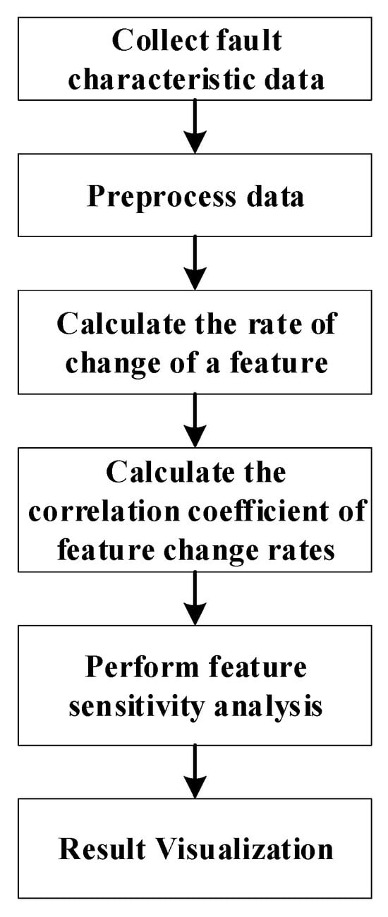
Figure 7. Flowchart of sensitivity analysis of fault characteristics based on correlation analysis approach.

Based on the aforementioned process, the sensitivity of statistical indicators for frequency response curve features under different fault conditions can be determined. Finally, suitable features for fault classification are selected based on their sensitivity levels. Next, the sensitivity of different frequency response curve features under various fault types is analyzed, and selections are made based on these feature variations.

Based on the above analysis, the absolute sum of logarithmic errors, correlation coefficient, absolute difference, spectral deviation, Euclidean distance, minimum-maximum ratio, and sum-of-squares ratio error are selected as highly sensitive features. These features demonstrate high sensitivity across different fault types and effectively reflect fault information. To further enhance fault diagnosis accuracy, feature weighting calculations and fusion can be performed by integrating characteristics such as the rate of change of the major axis, rate of change of the minor axis, and rate of change of the tilt angle from the ΔU-I trajectory curve. Feature fusion allows for the full utilization of each feature’s strengths, constructing a more comprehensive and sensitive multimodal feature representation system that provides more reliable raw data for fault diagnosis.

3.2.3. Construction of a Highly Sensitive Multimodal Feature System

In Section 3.2.2, although sensitivity analysis was performed on features under different curves and highly sensitive features were selected, these features were obtained based on distinct characteristic curves. Therefore, further feature fusion is required. This study employs Principal Component Analysis (PCA) to process feature data from both the impulse response method and ΔU-I trajectory, achieving feature fusion and feature weight calculation. This subsection first standardizes the feature data from both methods. PCA is then applied to the standardized data for dimensionality reduction, extracting principal components and calculating their weights. This process yields a matrix integrating features from both methods, as illustrated in the flowchart of Figure 8.

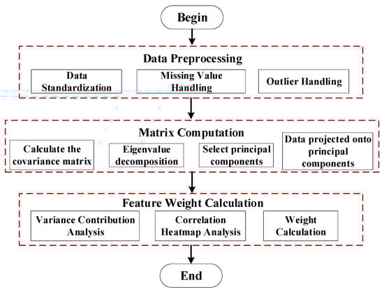
Figure 8. PCA-based high sensitivity multimodal feature system construction process.

The objective of PCA is to retain key information in the data by selecting principal components with greater variance. In feature weight calculation, PCA can effectively integrate frequency response curve features and ΔU-I trace curve features, thereby assigning appropriate weights to each feature. Feature preprocessing is a fundamental step, particularly for multidimensional, multi-type data, where normalization is crucial for subsequent PCA analysis. The commonly used method for standardization is Z-Score normalization. Assuming the original dataset is X = [X₁, X₂, X₃, …, X_m], where each X_i represents the i-th feature, the standardized data matrix becomes X_std. After standardization, each feature will have a mean of 0 and a standard deviation of 1. Subsequently, the covariance matrix Σ is calculated for the standardized dataset X_std to measure the correlations between different features.

Subsequently, the covariance matrix Σ undergoes eigenvalue decomposition to yield eigenvalues and eigenvectors. The eigenvalues λ₁, λ₂, …, λ_m of the covariance matrix represent the contribution of each principal component to the data variance, while the eigenvectors v₁, v₂, …, v_m denote the principal component directions in the new feature space. The eigenvalue decomposition process can be achieved by solving the following equation, as shown in Equation (12), where λ_i is the i-th eigenvalue and v_i is the i-th eigenvector.

$$\Sigma v_i={\lambda }_i{v}_i$$

(12)

Select the first few eigenvectors with the largest eigenvalues as the basis vectors for the new feature space. These principal components correspond to the largest variance in the data and retain most of the information from the original data. The top k principal components are typically selected based on the cumulative variance contribution p, as shown in Equation (13).

$$p={\displaystyle \frac{{\Sigma }_{i=1}^k{\lambda }_i}{{\Sigma }_{i=1}^m{\lambda }_i}}$$

(13)

If the cumulative contribution rate p exceeds 95%, it is considered that these k principal components are sufficient to retain most of the information in the original data. These principal components will be used to reconstruct the data space, preserving the primary information of the data.

After completing PCA dimensionality reduction, the next critical step is to calculate the comprehensive weights of each feature based on the results and use them to construct a highly sensitive multimodal feature system. PCA utilizes the combination of eigenvalues and eigenvectors to reveal the contribution levels of original features within principal components. To quantify the importance of each feature within the overall diagnostic system, their weights can be calculated as follows: First, square the coefficient of each feature in each principal component; then multiply this value by the corresponding eigenvalue of the principal component to measure its weighted contribution; finally, sum the weighted results across all principal components to obtain the overall weight for that feature. This method not only highlights the recognition capability of primary features but also suppresses interference from redundant information. The detailed calculation formula is provided in Equation (14),

$$w_i={\displaystyle \sum _{k=1}^m{v_{ik}}^2·{\lambda }_k}$$

(14)

where w_i is the weight of the i-th feature, v_ik is the coefficient of the i-th principal component in the k-th feature, λ_k is the eigenvalue of the k-th principal component (variance contribution rate), and m is the number of principal components selected.

After completing feature selection and weight adjustment, the features can be weighted and fused according to their respective weights to form the final feature matrix. The feature weight values for multimodal features are shown in Table 3.

Table 3. Feature weight values for multimodal features.

Name	Weight Value	Name	Weight Value
Logarithmic error absolute sum	0.1011	Minimum-to-maximum ratio	0.0946
Correlation coefficient	0.0912	Sum-to-square ratio error	0.1012
Absolute difference	0.0946	Major axis	0.0923
Spectral deviation	0.0979	Minor axis	0.0990
Euclidean distance	0.0957	Inclination angle	0.0968

Finally, the features were weighted and fused based on their respective weight values to form a representative composite feature vector. This highly sensitive feature matrix not only enhances information complementarity across different modalities but also provides more discriminative input data for subsequent AI-based fault classification models. Compared to traditional single-feature or empirically selected approaches, this strategy demonstrates superior adaptability in improving diagnostic accuracy and model efficiency.

4. Diagnosis of Winding Deformation Faults

4.1. Diagnosis of Winding Deformation Faults Based on the TCN-BiGRU-PHA Model

The proposed TCN-BiGRU-PHA (Physical-guided Hierarchical Attention) model integrates TCN’s time-series feature extraction capabilities, BiGRU’s bidirectional information utilization, and the attention mechanism’s focus on key features. By incorporating physical prior knowledge, the model outputs align more closely with physical laws, enhancing interpretability and credibility. This model architecture effectively addresses the complex data processing demands in winding deformation fault diagnosis, improving diagnostic accuracy and reliability.

4.1.1. Fundamental Principles

Time Convolutional Networks (TCNs) are a type of convolutional neural network designed for processing time-series data. TCNs utilize one-dimensional convolutional layers to extract local features within time series and employ dilated convolutions to capture long-term dependencies. Their core principle involves leveraging convolutional layers to identify patterns in time series, thereby effectively handling both local and long-term dependencies inherent in time-series data. The efficiency of TCNs lies in their ability to circumvent the vanishing gradient problem commonly encountered by traditional recurrent neural networks when processing long-term sequence data. Simultaneously, they leverage the parallel computation capabilities of convolutional layers to accelerate both model training and inference processes, with dilated convolutions serving as their core component.

The bidirectional gated recurrent unit is a bidirectional recurrent neural network that combines forward and backward gated recurrent units. BiGRU can simultaneously consider both forward and backward information in time series, thereby capturing dependencies within the sequence more comprehensively. Although the bidirectional structure increases computational overhead to some extent and imposes higher demands on hyperparameter tuning, these costs are acceptable and worthwhile given the resulting enhancement in feature representation capabilities. Therefore, incorporating BiGRU into fusion network models helps further uncover deep-level dependency information within sequence data, providing more precise decision support for fault diagnosis.

Attention mechanisms are algorithms that simulate human attention processes. They not only enable models to automatically focus on critical information by assigning different weights to inputs across various time steps, but also dynamically adjust the level of attention paid to different input features. By calculating attention scores and weights, the attention mechanism effectively filters information, enhances the model’s focus, and thereby improves prediction accuracy. Its advantages lie not only in enabling the model to concentrate on important parts of the sequence and enhance its ability to extract key information, but also in providing interpretability to the model, aiding in understanding its decision-making process.

4.1.2. Dataset and Experimental Protocol

The transformer winding deformation fault sample dataset constructed in this study is derived from an experimental platform, comprising measured and simulated data for three typical faults: inter-disc short circuit, radial deformation, and axial deformation. The measured data are obtained via physical simulation on the experimental platform, while the simulated data are generated through simulations of an equivalent circuit model of the transformer winding. By comparing and validating against the characteristics of typical fault cases provided by power grid companies, four sets of multimodal fault sample datasets integrating both experimental and simulated data have been established. The simulated data effectively fill the sample gaps for extreme operating conditions and complex coupled faults, and the distribution of the sample data is presented in Table 4. After time-frequency domain feature extraction and normalization, all samples are combined with the high-sensitivity feature weight assignment strategy proposed in Section 3.2.3 to form a hierarchical, highly sensitive multimodal feature set with physical interpretability. The collaborative validation of measured and simulated data not only expands the coverage of the sample size but also reveals the fault mechanism and the mapping laws between electromagnetic and mechanical characteristics through the simulated data. This provides a more comprehensive data foundation for constructing a physics-informed fault diagnosis model, significantly enhancing the engineering applicability of fault features and the reliability of diagnosis.

Table 4. Performance comparison of different models.

Fault Type	Sample Count	Fault Type Code
Winding without Fault	400	1
Inter-disc Spacing Variation	400	2
Radial Deformation	400	3
Axial Deformation	400	4

In this study, the dataset is partitioned into the training set, validation set, and test set at a ratio of 70%:15%:15%, with specific scales as follows: 1050 samples for the training set, 225 samples for the validation set, and 225 samples for the test set. During the partitioning process, the principle of “measured values from the same physical experiment shall not appear simultaneously in the training set and the test set” is strictly observed: all measured data generated by each physical experiment are treated as an independent unit and assigned entirely to either the training set, validation set, or test set. This avoids the artificial inflation of diagnostic accuracy caused by the cross-set distribution of data from the same experiment, and ensures that the evaluation of the model’s generalization ability using the test set is objective and authentic.

4.1.3. Model Construction and Training

This study proposes a deep learning model, TCN-BiGRU-PHA, that integrates physical prior knowledge. Its core innovation lies in establishing a full-chain physical constraint mechanism spanning from feature extraction to decision output, as illustrated in Figure 9. Figure 9 illustrates the three-level architecture of the TCN-BiGRU-PHA model: The TCN module extracts the local temporal features of the frequency response curve through dilated convolution; the BiGRU module captures the long-term dependencies of the Lissajous figure trajectory in both directions; the PHA mechanism dynamically weights multi-modal features based on physical priors. This model integrates the parallel computing efficiency of TCN, the sequence modeling capability of BiGRU, and the focusing characteristic of attention, and finally outputs the fault classification result through the fully connected layer. The input variable X_n of the TCN module is a 10-dimensional time-series sequence of high-sensitivity multi-modal feature vectors fused by principal component analysis (PCA) with weighted integration.

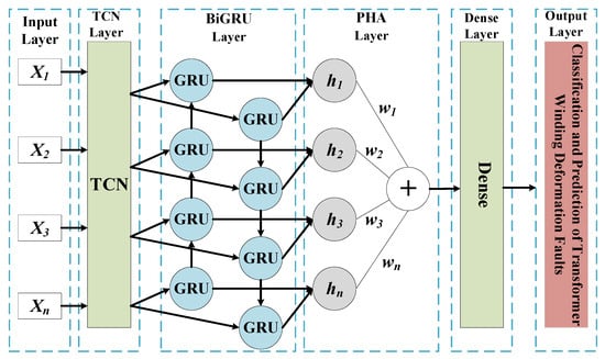
Figure 9. Structure of the TCN-BiGRU-PHA model.

This model incorporates physical prior knowledge by building upon TCN, BiGRU, and attention mechanisms, enabling more effective processing of data with physical constraints through a three-stage processing architecture. Its mathematical representation can be formalized as shown in Equation (15).

$$\mathcal{M}\left(X\right)={\mathcal{F}}_{PHA}\left({\mathcal{F}}_{TCN}\left(X_{FRA}\right)\oplus {\mathcal{F}}_{BiGRU}(X_{Traj})\right)$$

(15)

The temporal convolutional network module serves as the fundamental feature extractor, capturing local patterns of high-frequency response features through multiple layers of dilated causal convolutions. The physically constrained TCN module, enhanced based on spatio-temporal convolutional networks, consists of three cascaded residual blocks. Each residual block contains: a dilated causal convolution layer, a physically sensitive normalization layer, and gradient-constrained skip connections, as shown in the following equations.

$$y_t={\displaystyle \sum _{k=0}^{K-1}{w}_k·x_{t-d·k}}$$

(16)

$${\widehat{h}}_i=\gamma ·{\displaystyle \frac{h_i-\mu (w\odot H)}{\sigma (w\odot H)}}+\beta$$

(17)

$$z_{out}=\alpha ·f_{1\times 1}(z_{in})+(1-\alpha )\mathcal{F}(z_{in})$$

(18)

At the first layer of each residual block, a dilated causal convolution is implemented, with its discretization calculation shown in Equation (16). The dilation factor is configured hierarchically according to the expansion coefficient d = 21 for the l-th layer, following the exponential sequence [1, 2, 4, 8, 16, 32]. In the actual implementation, parameters with a kernel size of 3 × 3 and 256 filter groups are adopted to ensure the ability to capture cross-scale temporal patterns. Feature-weighted normalization is introduced after convolution, adjusting the activation distribution formula via Equation (17). Here, w denotes the feature initial weight vector determined in Section 3.2.3, and ⊙ represents the Hadamard product. This operation grants higher-sensitivity features a larger gradient propagation coefficient. The residual path employs the enhanced connection mechanism defined by Equation (18), where f_1×1 denotes dimension-aligned convolution, α = exp(−λ·we) represents the adaptive decay coefficient, and we is the mean of the current layer’s feature weights. When w falls below the preset feature weight threshold, gradient decay (λ = 5) is triggered to suppress overfitting risks associated with low-value features.

The network weights are initialized by convolving the fault sensitivity matrix $S\in {ℝ}^{d\times d}$ with the convolutional kernel, enabling the model to perform feature selection based on physical principles. The element S_i,j is calculated from the mutual information entropy between feature F_i and fault type c_j, as shown in Equation (19). The parameters of the first-layer convolutional kernel require probabilistic sampling to establish an explicit link between physical mechanisms and network parameters.

$$\begin{array}{l}{S}_{i,j}={\displaystyle \frac{I(F_i;c_j)}{{\displaystyle {\sum }_{k=1}^{n}I(F_i;c_j)}}}\\ I(X;Y)={\displaystyle \sum _{x\in X}{\displaystyle \sum _{y\in Y}p(x,y)\log \frac{p(x,y)}{p(x)p(y)}}}\end{array}$$

(19)

To address the issue of rapid decay in physical feature memory in traditional GRUs, the model proposed in this paper incorporates a forgetting gate bias term with physical weight regulation. The forward propagation process can be decomposed as shown in Equation (20).

$$\begin{array}{c}{z}_t=\sigma (W_z[h_{t-1},x_t])\\ r_t=\sigma (W_z\left[h_{t-1},x_t\right]+\log (1+w_j))\\ {\tilde{h}}_t=\tanh (W·\left[r_t\odot h_{t-1},x_t\right])\\ h_t=(1-z_t)\odot h_{t-1}+z_t\odot {\tilde{h}}_t\end{array}$$

(20)

Here, $w_j\in ℝ$ represents the feature weight vector, while the $\log (1+w_j)$ transformation ensures numerical stability. By injecting feature weights into the forgetting gate in logarithmic form, the model enhances memory retention for key features. This design endows the model with the following characteristics: reduced forgetting gate bias for high-weight features, prolonging their memory retention period; accelerated forgetting rate for low-weight features, suppressing noise interference.

The attention mechanism guided by physical prior knowledge dynamically adjusts the weights of frequency-response and trajectory features to achieve complementary advantages between the two. The PHA module consists of time-feature dual-granularity attention and physical mask constraints. Time attention primarily focuses on fault-sensitive time periods, as formulated in Equation (21).

$${\alpha }_t^{time}=soft\max ({\displaystyle \frac{Q·(K\odot E_f)}{\sqrt{d_k}}})$$

(21)

Here, E_f denotes the frequency-domain energy. Feature attention is employed to enhance physically sensitive features, with its formula shown in Equation (22).

$${\beta }_j^{feat}=sigmoid(W_{\beta }·h_j)·M_{j,c}$$

(22)

Define the feature-fault correlation matrix as M ∈ {0, 1}d × C. When feature i is sensitive to fault c, M_ic = 1. The final attention output is given by Equation (23).

$$h_{fusion}={\displaystyle \sum _{t=1}^T{\alpha }_t^{time}\odot }{\displaystyle \sum _{j=1}^{10}{\beta }_j^{feat}{h}_{j,t}}$$

(23)

The PHA module uses frequency-domain energy as the modulation signal for temporal attention, ensuring higher weights are assigned at moments of sudden changes in resonance frequency. Additionally, a hard feature selection is implemented via a fault-feature correlation matrix, permitting only physically correlated features to participate in the final decision. Through this combined approach, the TCN-BiGRU-PHA model fully leverages the efficient feature extraction capability of TCN, the bidirectional sequence modeling capability of BiGRU, and the dynamic feature selection capability of the attention mechanism, thereby achieving superior performance in fault diagnosis tasks.

The transformer winding deformation fault sample dataset constructed in this study was obtained from an experimental platform, comprising measured data from three typical fault types: cake-to-cake spacing variation, radial deformation, and axial deformation. Through comparative validation with characteristic features from typical fault cases provided by power grid companies, a dataset containing three sets of multimodal fault samples was established. After undergoing time-frequency domain feature extraction and normalization processing, a high-sensitivity feature weighting allocation strategy was applied to form a hierarchical, high-sensitivity multimodal feature system with physical interpretability.

During the training process of deep learning models, learning rate scheduling and dynamic batch size adjustment serve as two critical parameter optimization techniques. Their synergistic effects significantly enhance training efficiency and model performance. The learning rate employs a cosine annealing scheduling strategy, with an initial value of 3 × 10⁻⁴ and a minimum value of 1 × 10⁻⁶. The core principle of this strategy is to achieve rapid convergence during the early training phase and perform fine-tuning in the later stages through periodic adjustments to the learning rate. The batch size is fixed at 64. This setting balances training efficiency and stability. Under a fixed number of iterations, the fixed-batch strategy reduces training randomness and enhances the reproducibility of model convergence. Figure 10 shows the accuracy curve and network loss curve of the model during training.

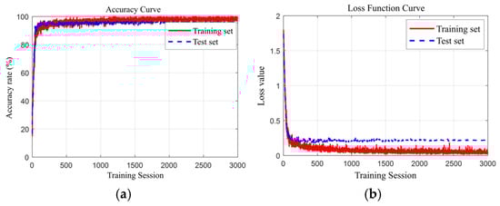
Figure 10. TCN-BiGRU-PHA model training accuracy and network loss variation. (a) Accuracy rate (b) Network Loss.

From the accuracy curve in Figure 10a, it can be observed that both the training set and test set accuracy rapidly increase as the number of training iterations grows, stabilizing after reaching a certain number of iterations. This phenomenon indicates that the model performs well on both training and test data, with no significant signs of overfitting or underfitting.

The loss function curve in Figure 10b further validates the above conclusion. The network loss curve demonstrates that both the training set and test set losses decrease significantly as the number of training iterations increases, eventually stabilizing after a certain number of iterations.

In summary, the model demonstrated strong learning capabilities and generalization performance throughout both training and testing phases. Detailed analysis of the training process yields the following key conclusions:

• Throughout the entire training process, the accuracy and loss curves for the training and validation sets remained consistently aligned, with a gap of less than 2%. This indicates that the model did not exhibit overfitting at any stage of training.
• The model achieved over 95% accuracy on the validation set, with the training set’s loss function ultimately stabilizing at 0.09 and the validation set’s loss function stabilizing at 0.20. This demonstrates that the model’s loss function gradually converged and remained stable during training, proving the training process to be both effective and stable.

4.1.4. Model Performance Comparison Analysis

After completing the training and validation process of the TCN-BiGRU-PHA model, ablation experiments were conducted to thoroughly evaluate the effectiveness of the physics-guided mechanism. This experiment compared the performance of different model combinations in transformer fault diagnosis scenarios, aiming to analyze the impact of each module on multimodal feature fusion capabilities and provide a basis for model optimization.

In the transformer fault diagnosis scenario that integrates statistical indicators of frequency response curves and geometric parameters of ΔU-I trajectories, the multi-modal feature fusion capability of different algorithms directly affects the classification accuracy. The TCN-BiGRU-PHA model achieves the optimal overall performance, as evidenced by the highest proportion of diagonal elements in its confusion matrix. It particularly excels in identifying complex faults such as inter-disc short circuits and axial deformation. This high accuracy stems from the TCN module’s effective extraction of frequency response curve features, especially its sensitivity to energy concentration in low-frequency bands and resonance peak shifts. Meanwhile, the integration of the BiGRU module further enhances the model’s ability to capture the temporal dynamics of ΔU-I trajectory features. Additionally, PHA strengthens the model’s adaptability across diverse scenarios by dynamically adjusting feature weights, thereby ensuring classification accuracy and robustness.

As can be observed from the accuracy rates presented in the Table 5, the TCN-BiGRU-PHA model significantly outperforms other models in terms of final performance. This not only verifies the complementary role of trajectory features to frequency response features and the importance of frequency response features in fault diagnosis, but also demonstrates that the physically guided attention mechanism effectively enhances the feature fusion effect. Through the physically guided attention mechanism, the TCN-BiGRU-PHA model achieves deep fusion of frequency response features and trajectory features, which mainly includes the following three aspects: (1) Frequency response features exhibit high sensitivity—convolutional kernels are configured via a physical sensitivity matrix to enable the model to quickly capture fault features; (2) Trajectory features possess strong anti-interference capability—a logarithmic gating mechanism is employed to enhance the memory capacity of key trajectory features; (3) The attention mechanism yields remarkable effects—spatiotemporal dual-dimensional attention is adopted to realize synergistic optimization of multi-modal features.

Table 5. Comparison of the performance of different models after ablation experiments.

Model	TCN-BiGRU	BiGRU-PHA	TCN-PHA	TCN-BiGRU-PHA
accuracy	93.4%	90.8%	92.8%	97.3%

Specifically, among all models, the Support Vector Machine (SVM) model achieves an accuracy of 85.7%, the Multi-Layer Perceptron (MLP) model 89.4%, the K-Nearest Neighbor (KNN) model 83.9%, the ResNet-50 model 94.7%, the 1D-Convolutional Neural Network (1D-CNN) 91.5%, and the Long Short-Term Memory (LSTM) model 93.1%. By contrast, the hybrid model TCN-BiGRU-PHA delivers the optimal performance with an accuracy of 97.3% (Table 6). This clear performance gradient reveals the evolution and improvement from traditional machine learning to deep learning, and further to hybrid architecture models in the task of multi-modal temporal fault diagnosis. Among traditional models, the performance of SVM is highly dependent on the selection of kernel functions and parameter tuning. In multi-modal high-dimensional temporal scenarios, commonly used kernels such as the Radial Basis Function (RBF) may struggle to balance inter-modal differences and temporal dependencies, which tends to result in overfitting or underfitting. As a basic neural network, MLP possesses a certain degree of non-linear fitting capability, yet it exhibits weak performance in modeling temporal structures, is prone to overfitting, and has limited generalization ability. KNN treats all features equally while ignoring the temporal relationships among them, making it vulnerable to interference from noise and irrelevant features in complex multi-modal diagnosis tasks.

Table 6. Performance comparison of different models.

Model	SVM	MLP	KNN	ResNet-50	1D-CNN	LSTM	TCN-BiGRU-PHA
Accuracy	85.7%	89.4%	83.9%	94.7%	91.5%	93.1%	97.3%
Precision	84.9%	88.8%	83.2%	94.3%	91.0%	92.6%	96.9%
Recall	85.5%	89.2%	83.8%	94.5%	91.4%	93.0%	97.2%
F1 Score	85.2%	89.0%	83.5%	94.4%	91.2%	92.8%	97.0%

In comparison, deep learning models demonstrate significant advantages: ResNet-50 effectively extracts deep spatial features through its residual structure, but has limitations in temporal modeling; 1D-CNN can capture local temporal patterns, yet lacks the capacity to model long-range dependencies; although LSTM is specialized in sequence modeling, it has limited ability to capture synchronous interactions across multiple modalities. On the other hand, the TCN-BiGRU-PHA hybrid model captures long-term dependencies via the Temporal Convolutional Network (TCN), enhances contextual understanding by integrating the Bidirectional Gated Recurrent Unit (BiGRU), and introduces the Parallel Hybrid Attention (PHA) mechanism to realize dynamic weight allocation of multi-modal features. Consequently, it achieves superior feature fusion and pattern recognition in multi-modal temporal fault diagnosis, significantly improving diagnostic accuracy and robustness, and exhibits stronger adaptability in the collaborative modeling of cross-modal temporal features.

4.2. Fault Diagnosis Performance Analysis

As described in Section 3, the pulse frequency response method and ΔU-I trajectory method are two commonly used techniques in transformer winding fault diagnosis, each possessing distinct advantages and limitations. The pulse frequency response method can capture resonance point shifts caused by minor faults but has limited diagnostic capability for complex faults; The ΔU-I trajectory method reflects changes in winding electrical parameters through time-domain waveform analysis, demonstrating strong interference resistance but lower sensitivity in detecting minute faults. To overcome these limitations, this paper proposes the TCN-BiGRU-PHA model. By deeply integrating frequency response features and trajectory features, it constructs a highly sensitive multimodal feature space that achieves complementary advantages between the two methods. Features from different modalities are dynamically fused through a physically hierarchical attention module. Under identical training iterations, the diagnostic performance of fault detection using combined modal features from the model trained in Section 4.1 is evaluated, with results presented in Table 7.

Table 7. Fault diagnosis performance with different modal feature inputs.

Feature Type	Dimension/Modality	Accuracy	Characteristics
Frequency Response Characteristics	7-dimensional/Single-modal	92.1%	High sensitivity, capable of detecting minor faults
Trajectory Characteristics	3-dimensional/Single-modal	87.5%	Strong anti-interference capability, high stability
Multimodal Fusion Features	10-dimensional/Single-modal	97.3%	Balances sensitivity and anti-interference capability

Analysis of the above data reveals that the fusion of frequency response features and trajectory features achieves complementary advantages. The accuracy of the multi-dimensional feature model reaches 97.3%, representing an improvement of 5.2% to 9.8% over single-feature models, thereby enhancing the accuracy of fault diagnosis. Multimodal feature fusion maintains high accuracy by integrating the strengths of both approaches. This is not only because the high sensitivity of frequency response features captures subtle changes in frequency response curves caused by minor faults through metrics like absolute logarithmic error and ratio of squared errors, but also due to trajectory features’ strong interference resistance. Trajectory features enhance the model’s adaptability to complex operating conditions through characteristics like major axis, minor axis, and tilt angle. This demonstrates that the multimodal feature space offers advantages over single-modal feature models in terms of increased information content and enhanced diagnostic capabilities. Finally, through a physical hierarchical attention mechanism, the weights of frequency response and trajectory features are dynamically adjusted. When capturing minor faults, the weight of frequency response features increases to 65%, while under complex operating conditions, the weight of trajectory features rises to 55%.

Feature fusion achieves complementary advantages between modalities on this foundation. Under various interference conditions, the accuracy of the fusion model consistently remains above 90%, fully validating the effectiveness and practicality of the fusion strategy. Frequency response features exhibit high sensitivity to minute structural deformations, while trajectory features demonstrate robust resilience against multiple external disturbances. Through fusion, the two feature types compensate for each other’s limitations: trajectory features effectively suppress the excessive sensitivity of frequency response features to noise in the high-frequency range, while the energy distribution information from frequency response features corrects measurement jitter in trajectory parameters at low frequencies. This significantly enhances the overall performance of the model.

In summary, multimodal fusion strategies demonstrate significant advantages over single-feature approaches, not only enhancing diagnostic accuracy but also improving the model’s adaptability under complex operating conditions. Furthermore, the online joint analysis method offers faster response times, stronger real-time capabilities, and easier deployment compared to traditional offline analysis methods. It is particularly well-suited for continuous monitoring and intelligent diagnosis of power equipment operating conditions, ensuring the system’s fault identification capability during dynamic operation.

5. Conclusions

5.1. Summary of This Article’s Work

This paper addresses the issues of insufficient sensitivity in online detection of mechanical deformation in transformer windings. It proposes a high-sensitivity multimodal joint analysis method integrating the pulse frequency response method with the ΔU-I trajectory method, and constructs an intelligent fault identification model based on deep neural networks. The main research findings are as follows:

• An online measurement platform suitable for simulating multiple types of winding deformation experiments was established. Three representative fault experiments were conducted to obtain characteristic bimodal response data, verifying the complementary characteristics of the IFRA and ΔU-I trajectory methods at the frequency response and phasor trajectory levels.
• An initial feature set is constructed based on frequency response characteristics and current-voltage trace profiles. PCA is applied to perform feature sensitivity analysis and redundancy elimination, establishing a high-sensitivity feature metric system that provides critical variables for subsequent modeling.
• Design and implement a deep learning diagnostic model integrating TCN, BiGRU, and PHA modules. This model combines time series modeling capabilities with attention-based selection mechanisms, demonstrating superior performance in processing complex nonlinear time-varying data. It significantly enhances fault identification accuracy and interference resistance.
• Analysis of the results indicates that the combined analysis method demonstrates superior stability and generalization capabilities compared to single-feature-source approaches. The ΔU-I curve exhibits heightened sensitivity to interturn short circuits at low frequencies, while IFRA reveals greater responsiveness to structural changes at medium-to-high frequencies. Integrating these two methods facilitates comprehensive monitoring of winding conditions, underscoring the critical importance and necessity of feature fusion.

This study provides theoretical support and practical pathways for achieving high-performance, intelligent online monitoring of transformer winding deformation. Subsequent research may further incorporate multi-source information fusion, few-shot learning, and transfer learning strategies to enhance model adaptability and engineering applicability.

5.2. Limitations and Future Work

This study conducted experiments based on a model transformer. Although it effectively simulated the structural characteristics of the windings of actual transformers, there remains a certain gap from the complex operating conditions of large-scale real-world transformers. Future work will be carried out in the following aspects:

• Verification of applicability to multiple transformer models: Deploy the system on real transformers with different capacities and voltage levels to verify the model’s generalization ability and adaptability.
• On-site environmental interference suppression strategies: Further optimize signal acquisition and feature extraction methods targeting factors such as on-site electromagnetic interference, temperature variations, and load fluctuations.
• System integration and real-time performance optimization: Develop an embedded diagnostic device to improve the real-time performance of the algorithm and ensure the response speed and stability of online monitoring.
• Transfer learning and few-shot fault diagnosis: Explore few-shot learning and transfer learning methods to reduce reliance on large volumes of labeled data and enhance engineering practicality.

References

- Abu-Siada, A.; Mosaad, M.I.; Kim, D.W.; El-Naggar, M.F. Estimating Power Transformer High Frequency Model Parameters Using Frequency Response Analysis. IEEE Trans. Power Deliv. 2020, 35, 1267–1277. [Google Scholar] [CrossRef]
- Lin, J.; Ma, J.; Zhu, J.G.; Cui, Y. A Transfer Ensemble Learning Method for Evaluating Power Transformer Health Conditions with Limited Measurement Data. IEEE Trans. Instrum. Meas. 2022, 71, 3513910. [Google Scholar] [CrossRef]
- Liu, J.; Li, Z.; Zhou, Y. Transformer windings based on leakage field and ICOA-ResNet early fault diagnosis. Power Syst. Prot. Control 2024, 52, 99–110. [Google Scholar] [CrossRef]
- Cao, C.; Xu, B.W.; Li, H. Composite monitoring method for the state of transformer winding deformation based on vibration and reactance information. High Volt. Eng. 2022, 48, 1518–1530. [Google Scholar] [CrossRef]
- Chen, Y.; Zhao, Z.; Liu, J.; Tan, S.; Liu, C. Application of Generative AI-based Data Augmentation Technique in Transformer Winding Deformation Fault Diagnosis. Eng. Fail. Anal. 2024, 159, 108115. [Google Scholar] [CrossRef]
- C57.149-2012; IEEE Guide for the Application and Interpretation of Frequency Response Analysis for Oil-Immersed Transformers. IEEE: Piscataway, NJ, USA, 2013. [CrossRef]
- Zhou, H.; Lu, L.; Wang, G.; Su, Z. A New Validity Detection Method of Online Status Monitoring Data for Power Transformer. IEEE Access 2024, 12, 16095–16104. [Google Scholar] [CrossRef]
- Shanmugam, N.; Madanmohan, B.; Rajamani, R. Influence of the Load on the Impulse Frequency Response Approach Based Diagnosis of Transformer’s Inter-Turn Short-Circuit. IEEE Access 2020, 8, 39454–39463. [Google Scholar] [CrossRef]
- Ferreira, R.S.d.A.; Picher, P.; Meghnefi, F.; Fofana, I.; Ezzaidi, H.; Volat, C.; Behjat, V. Reproducing Transformers’ Frequency Response from Finite Element Method (FEM) Simulation and Parameters Optimization. Energies 2023, 16, 4364. [Google Scholar] [CrossRef]
- Zhao, Z.; Yao, C.; Li, C.; Long, Y.; Chen, X.; Liao, R. Method for obtaining the impulse frequency response curves of power transformer winding deformation based on short time Fourier transform. High Volt. Eng. 2016, 42, 241–247. [Google Scholar] [CrossRef]
- Chen, X.; Zhao, Z.; Guo, F.; Tan, S.; Wang, J. Diagnosis method of transformer winding mechanical deformation fault based on sliding correlation of FRA and series transfer learning. Electr. Power Syst. Res. 2024, 229, 110173. [Google Scholar] [CrossRef]
- Qian, G.; Yang, K.; Hu, J.; Liu, H.; He, S.; Zou, D.; Dai, W.; Wang, H.; Wang, D. Fault Diagnosis Method for Transformer Winding Based on Differentiated M-Training Classification Optimized by White Shark Optimization Algorithm. Energies 2025, 18, 2290. [Google Scholar] [CrossRef]
- Li, C.; Zhu, T.; Yao, C.; Xia, Q.; Mi, Y.; Zhao, Z. Online diagnosis method for transformer winding deformation based on characteristic of figure constructed by voltage and current. High Volt. Eng. 2018, 44, 3532–3539. [Google Scholar] [CrossRef]
- Wang, X.; Teng, Y.; Shi, P.; Zhang, W.; Chen, B.; Bai, J.; Du, X.; Gou, J.; Hu, P. A hybrid islanding detection method based on the Lissajous Pattern and impedance for grid-forming energy storage inverter. Energy Storage Sci. Technol. 2025, 14, 1299–3109. [Google Scholar] [CrossRef]
- Behjat, V.; Vahedi, A.; Setayeshmehr, A.; Borsi, H.; Gockenbach, E. Diagnosing Shorted Turns on the Windings of Power Transformers Based Upon Online FRA Using Capacitive and Inductive Couplings. IEEE Trans. Power Deliv. 2011, 26, 2123–2133. [Google Scholar] [CrossRef]
- Abu-Siada, A.; Islam, S. A Novel Online Technique to Detect Power Transformer Winding Faults. IEEE Trans. Power Deliv. 2012, 27, 849–857. [Google Scholar] [CrossRef]
- Zhang, Y.; Kang, H.; Wang, Q. MMFDetect: Webshell Evasion Detect Method Based on Multimodal Feature Fusion. Electronics 2025, 14, 416. [Google Scholar] [CrossRef]
- Han, H.; Meng, Y.; Wu, X.; Li, X.; Qiao, J. A Transfer Learning-Based Multimodal Feature Fusion Model for Bearing Fault Diagnosis. IEEE Trans. Instrum. Meas. 2025, 74, 3530413. [Google Scholar] [CrossRef]
- Zhang, Z.; Deng, Y.; Liu, X.; Liao, J. Research on Fault Diagnosis of Rotating Parts Based on Transformer Deep Learning Model. Appl. Sci. 2024, 14, 10095. [Google Scholar] [CrossRef]
- Vatsa, A.; Hati, A.S. Insulation Aging Condition Assessment of Transformer in the Visual Domain Based on SE-CNN. Eng. Appl. Artif. Intell. 2024, 128, 107409. [Google Scholar] [CrossRef]
- Cui, J.; Kuang, W.; Geng, K.; Jiao, P. Intelligent Fault Diagnosis and Operation Condition Monitoring of Transformer Based on Multi-source Data Fusion and Mining. Sci. Rep. 2025, 15, 7606. [Google Scholar] [CrossRef]
- Yu, R.; Wang, R. Learning dynamical systems from data: An introduction to physics-guided deep learning. Proc. Natl. Acad. Sci. USA 2024, 121, 10. [Google Scholar] [CrossRef]
- Fu, R.; Su, T.; Li, M.; Wu, Y.; Ouyang, R.; Solina, D.; Cortie, M.; Zhang, T.; Hu, S.; Ren, Z. Physics-guided deep learning strategy for 2D structure reconstruction from diffraction patterns. Commun. Phys. 2025, 8, 221. [Google Scholar] [CrossRef]
- Rahimpour, H.; Mitchell, S.; Rahimpour, S. Online Monitoring of Power Transformers Using Impulse Frequency Response Analysis. In Proceedings of the 2017 Iranian Conference on Electrical Engineering (ICEE), Tehran, Iran, 2–4 May 2017; pp. 1390–1394. [Google Scholar]
- Zhao, X.; Yao, C.; Zhou, Z.; Li, C.; Wang, X.; Zhu, T.; Abu-Siada, A. Experimental Evaluation of Transformer Internal Fault Detection Based on V–I Characteristics. IEEE Trans. Ind. Electron. 2019, 67, 4108–4119. [Google Scholar] [CrossRef]
- DL/T 911-2016; Frequency Response Analysis on Winding Deformation of Power Transformers. National Energy Administration: Beijing, China, 2016.
Disclaimer/Publisher’s Note: The statements, opinions and data contained in all publications are solely those of the individual author(s) and contributor(s) and not of MDPI and/or the editor(s). MDPI and/or the editor(s) disclaim responsibility for any injury to people or property resulting from any ideas, methods, instructions or products referred to in the content. |
© 2025 by the authors. Licensee MDPI, Basel, Switzerland. This article is an open access article distributed under the terms and conditions of the Creative Commons Attribution (CC BY) license.