Chemical Looping Gasification with Microalgae: Intrinsic Gasification Kinetics of Char Derived from Fast Pyrolysis

Abstract

Chemical looping gasification (CLG) based on interconnected fluidized beds is a viable technology to produce a syngas stream for chemical and fuel production. In this work, microalgae are studied for use in the CLG process; more specifically, the intrinsic kinetics of char gasification have been analyzed, as it is important for the fuel conversion and design of reactor systems. Char produced from fast pyrolysis was used in a thermogravimetric analyzer (TGA) for intrinsic kinetics analysis, and measures were made to eliminate the interparticle and external particle gas diffusion. The effect of typical operational variables, such as temperature, concentration of gasification agents (H₂O and CO₂), and concentration of gasification products (H₂ and CO), were investigated. The TGA data is used to derive a suitable gasification model that can best fit the experimental data. The fitting with experiments then generates values of the model’s kinetics parameters. Based on the model and the kinetics values, the activation energies in the gasification with steam and CO₂ were calculated to be 43.3 and 91.6 kJ/mol, respectively. The model has a good capability in the prediction of the gasification profile with H₂O and CO₂ under a complex reacting atmosphere.

1. Introduction

Chemical looping gasification (CLG) is a novel technology for high-quality syngas production, where the gasifying air/O₂ and biomass are not mixed [1]. Therefore, CLG generates an undiluted syngas stream, and thus the conventional intense gas separation (like through cryogenic) is avoided naturally in the CLG process [2,3]. The syngas can then be used as an important building block for many synthesis processes [4], e.g., liquid fuel production through the Fischer–Tropsch process [5]. Green H₂ can also be generated from the CLG when the CO₂ is separated [6].

Figure 1 depicts the principle of the CLG technology. CLG has an air reactor, a fuel reactor, and an oxygen carrier that are used for transferring oxygen and heat from the air reactor to the fuel reactor [7,8]. The oxygen carrier consists of oxides of transition metals (MO) and practically exists in the form of natural ores, industrial by-products, and synthesized materials [9]. Upon the feeding of fuel to the fuel reactor, volatiles and char are generated through the decomposition reaction (1). The char is then gasified through reaction (2), and the gasification products (H₂ and CO) together with the volatiles reduce the oxygen carrier to a reduced state (M) through reaction (3). The oxygen carrier is then re-oxidized to MO by air in the air reactor through reaction (4). This oxidation reaction is exothermic, and the heat can be taken up by the oxygen carrier. So, when the oxygen carrier is circulated back to the fuel reactor, the sensible heat is also carried over and can balance the heat demand by the endothermic gasification [7]. Therefore, the oxygen carrier is also a heat carrier, and when the heat transferred is the same as the heat needed in the gasification, the system is autothermal. In autothermal conditions, some CO₂ will be generated, but the CO₂ is highly concentrated and thus amiable for carbon capture and subsequent storage (CCS). This is because the two CLG reactors have no gas exchange, and the syngas from the fuel reactor is not diluted by air-N₂ or oxygen that is commonly used in conventional gasification [10]. Therefore, the syngas and CO₂ separation from N₂ and O₂ in CLG is inherent and thus the associated energy penalty is low. CLG emerges as a novel technology for the production of syngas, which is an important precursor for the production of hydrogen, liquid fuels, and other energy vectors. When integrated with biomass carbon capture, the CLG becomes a bio-energy CCS (BECCS) technology. This means the process removes CO₂ from the atmosphere; thus, the overall net carbon emissions from the process are negative [11]. Microalgae are biomass and are promising for use in the CLG process. In addition to attaining negative carbon emissions, the use of microalgae in CLG can be implemented to produce third generation biofuels, which are more sustainable than the former two generations and are expected to take important roles in the world’s decarbonization goals [12].

$$\mathrm{F}\mathrm{u}\mathrm{e}\mathrm{l}\to \mathrm{V}\mathrm{o}\mathrm{l}\mathrm{a}\mathrm{t}\mathrm{i}\mathrm{l}\mathrm{e}\mathrm{s}+\mathrm{C}\mathrm{h}\mathrm{a}\mathrm{r}$$

(1)

$$\mathrm{C}\mathrm{h}\mathrm{a}\mathrm{r}+{\mathrm{H}}_2\mathrm{O}/{\mathrm{C}\mathrm{O}}_2\to \mathrm{S}\mathrm{y}\mathrm{n}\mathrm{g}\mathrm{a}\mathrm{s}\left({\mathrm{H}}_2+\mathrm{C}\mathrm{O}\right)$$

(2)

$$\mathrm{M}\mathrm{O}+\mathrm{S}\mathrm{y}\mathrm{n}\mathrm{g}\mathrm{a}\mathrm{s}+\mathrm{V}\mathrm{o}\mathrm{l}\mathrm{a}\mathrm{t}\mathrm{i}\mathrm{l}\mathrm{e}\mathrm{s}\to \mathrm{M}+{\mathrm{H}}_2\mathrm{O}+{\mathrm{C}\mathrm{O}}_2$$

(3)

$$\mathrm{M}+\mathrm{a}\mathrm{i}\mathrm{r}\to \mathrm{M}\mathrm{O}+\mathrm{d}\mathrm{e}\mathrm{p}\mathrm{l}\mathrm{e}\mathrm{t}\mathrm{e}\mathrm{d} \mathrm{a}\mathrm{i}\mathrm{r}$$

(4)

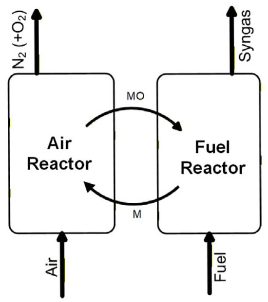
Figure 1. Principle of the CLG technology.

Microalgae are abundant raw materials for biofuel production, and they are highly efficient at photosynthesis, allowing them to grow quickly [13]. Unlike traditional feedstocks (food for first-generation and wood for second-generation biofuels), microalgae do not need farmland or forestland, and this avoids competitions with food and forestry industries [14]. Although microalgae are a main precursor for third-generation biofuel production, their high content of ash is considered as a “dirty” component which could provoke major challenges for use in many thermochemical processes [15]. The “dirty” ash can cause severe fouling and corrosion to the heat-exchange surfaces in conventional gasifiers, possibly leading to operational failures and other issues. But CLG can address this problem well and is particularly interesting for the gasification of microalgae. This is because the fuel conversion occurs in the fuel reactor and the heat-exchanger surfaces are placed in the air reactor. Therefore, the surfaces are free from aggressive ash species; hence, high-temperature corrosion could be avoided [16,17]. Moreover, CLG has many other advantages that are promising for solving some common issues in gasification processes, for example, suppressing tar formation, lowering energy penalty, and producing pure nitrogen gas stream [17,18].

Several works studied the microalgae–CLG process, but mostly with fixed-bed reactors and microreactors [19,20,21]. These studies have shown impressive results which are important for initiating microalgae–CLG studies with fluidized-bed reactors. Considering those promising results, Mei et al. [22] recently studied the microalgae–CLG process with several oxygen carriers in a fluidized bed reactor. In this previous work, several Fe- and Mn-based materials were evaluated, and some promising oxygen carriers were identified. The authors also observed a strong catalytic effect in the gasification due to the presence of alkali (K and Na) and alkaline earth (Ca) metals in the microalgae [22]. These components are strong catalysts for gasification and can greatly accelerate the rate of gasification. In the previous work, the catalysis on gasification is clearly seen at the stage close to the end of gasification. This interesting phenomenon indicates that the mechanism of catalysis on gasification may be different at the beginning and at the end of the gasification. This encourages us to carry out more studies to help understand the mechanisms behind it. In order to be able to design and understand a CLG process with microalgae, it is necessary to understand how both the volatiles and char are converted. In this work, the focus is on the latter, as the conversion rate governs the residence time of solids in the fuel reactor. By studying the kinetics of char conversion, it is possible to determine the rate of reaction and identify the rate-limiting mechanisms. This information is essential for use in optimizing reaction processes and in guiding reactor design and technology scale-up [23]. Chlorella microalga gasification kinetics was studied in a supercritical water gasification (SCWG) process, and the activation energies were reported to be around 46 and 238 kJ/mol [24]. The gasification kinetics of a Chlorella vulgaris and a Spirulina were also studied but with a distributed activation energy model (DAEM), this research found that the microalgae’s components greatly affect kinetics [25]. It was found the Chlorella vulgaris is easier to gasify as compared to the Spirulina [25]. The gasification of Chlorella vulgaris started at temperatures lower than 500 °C and has an activation energy of 500 kJ/mol, whereas the Spirulina gasification needs a higher temperature (>500 °C) and an activation energy higher than 500 kJ/mol. Similarly, a Chlorella vulgaris ESP-31 was studied for gasification with CO₂ [26], and the activation energy was 300–360 kJ/mol. It is obvious that the microalgae type has a great impact on gasification performance. In addition, the ash compositions in biomass were also commonly reported for their positive effect on gasification [27]. The presence of potassium and sodium in biomasses usually makes them gasify faster than fossil fuels, like petcoke and coal [28]. González–Vázquez et al. [29] studied the gasification kinetics of twelve biomasses and found that K, Na, and Mg components can promote gasification while the Si, P, and Ca components hinder the gasification. The positive effect of the alkalis can improve the gasification rate by 7–40 times. The effect is also observed in the authors’ later work with a bubbling fluidized bed reactor [30]. Moreover, the type and content of ash constitute (e.g., potassium) have shown clear effect on the profile of char gasification rate, and three types of rate evolution versus conversion (and thus the kinetics models) were observed when varying the K/(Si+P) ratio in biomasses [31]. The significant effect of potassium on biomass char gasification was also seen in a fluidized bed reactor, and when doped with potassium, a wood char gasified 3–5.5 times faster than the untreated char [32].

These studies have brought important apparent kinetics information on the catalytic effect of biomasses’ inherent alkali. This is crucial for the understanding of the gasification process, reactor design, process optimization, and reaction mechanism analyses. But the kinetics did not rule out the effect of external factors, like mass transfer and gas transport [33,34], and the kinetics data derived may be only suitable for those specific cases. So, this apparent kinetics may not be used directly in reactor modelling before performing certain processing. Conversely, intrinsic kinetics does not have this issue and can be used in reactor modelling straightforwardly [35]. Intrinsic kinetics present the core information of a chemical reaction and remove the effect of various external barriers, like mass and heat transport, and provide a pure measure of the reaction’s inherent chemical behaviour [36]. Intrinsic kinetics can be then combined with other rate-limiting factors, e.g., external mass transfer, to derive apparent kinetics and be used in broader scenarios [37]. Therefore, intrinsic kinetics is crucial for understanding the true rate of reactions. However, studies on intrinsic kinetics of char gasification (especially fast char that is normally seen in fluidized beds) are very limited or nonexistent for microalgae.

Fast char is char produced by fast pyrolysis at high temperatures. In this condition, the time of pyrolysis is very short; thus, the char’s porosity, surface morphology, and activity are very different as compared to slow char that is usually generated in a slow-heating process [38]. The fast char can keep most microstructure and physiochemical properties of the char right after its formation at high temperatures in fluidization systems. In a chemical looping process, fuel pyrolysis usually completes in 2–5 s [39]; thus, the kinetics of fast char can better approximate real gasification as compared to the slow char. This offers more useful information for process diagnostics, process optimization, and technology scale-up.

This work studies the intrinsic kinetics of microalgae gasification, and the fast char derived from a typical microalga is used throughout the gasification experiments. The results are expected to be used in understanding the previously observed unique fast gasification, especially at the final stage of gasification. The intrinsic kinetics analysis is performed by devising experiments in a way as to avoid mass transfer aspects in the TGA. This demands careful assessment of char–gas contact patterns which our group has significant experience with, and similar experiments have been performed previously in our group using other fuels.

2. Experimental

2.1. Microalgae and Char

Spirulina microalga, which is among the world’s most abundant microalgae, is used as the source of the fast char. The algae were from Brazil and received in powder of several micron-metres. Before their use for fast char preparation, they were granulated to particles to facilitate their use in a fluidized bed during the char preparation. The granulation was performed with a granulator (Eirich’s model EL1 Hardheim, Germany), using deionized water as the only binder (see Mei et al.) [22]. After the granulation, the granulates were dried naturally at room temperature and then sieved to particles in between 200 and 400 µm. A fluidized bed reactor [22] was used to rapidly devolatilize the microalgae to obtain the fast char particles. And the microalgae were placed in a wire-meshed chamber and immersed quickly in the fluidized bed under N₂ flow at 950 °C. In the reactor, the algae were pyrolyzed rapidly (<1 min), and at the end of pyrolysis, the chamber was cooled down quickly (<5 min) in N₂ to obtain the fast char. The fast char was then well-milled and homogenized with an agate mortar. After sieving, the particles with a size of 100–200 µm were used in the following TGA experiments for the kinetics analysis. A proximate and ultimate analysis of the Spirulina is displayed in Table 1 and this confirms the high volatile content in the original fuel; and the nitrogen and ash content is higher than the average level in most biomasses. The ash contains a high content of potassium (K), sodium (Na), and phosphorous (P), which can play the role of a catalyst to enhance the gasification [40].

Table 1. Proximate and ultimate and ash analyses of the Spirulina microalga and the fast char as produced as part of this work.

Proximate (%, as Received Basis)		Ultimate& Cl (%, Dry Basis)		ICP-AES Analysis d
Spirulina					Spirulina mg/kg Spirulina	Fast char mg/kg Char
Moisture	17.8	C	40.4	Ca	1465	9042
Ash	8.1	H	7.2	K	17,267	85,800
Volatiles	63.3	N	8.9	Mg	2856	16,628
Fixed carbon	10.8 a	S	0.6	Na	10,761	60,857
LHV(MJ/kg)	18	O b	34.7	P	8298	47,571
		Cl c	1.04	Si	728	4628

^a by the difference: 100-(moisture + ash + volatiles); ^b by the difference: 100-(C + H + N + S + A); ^c analyzed with ion chromatography (IC); ^d analyzed with inductively coupled plasma atomic emission spectroscopy (ICP-AES) technique.

2.2. Thermogravimetric Analysis

The char gasification experiments were carried out under various reacting conditions with the TGA (equipped with CI thermobalance, CI Precision, Salisbury, UK), as schemed in Figure 2. The TGA has two concentric quartz tubes (24 mm i.d. and 10 mm i.d.) placed in an electric oven. With this design, the gas entering the reactor can first be preheated in the external annulus before contacted with the sample at the bottom of the reactor. The char sample is held with layers of quartz wool in a wire-meshed platinum basket (approx. 14 mm wide and 8 mm high) and hung at the centre of the reactor. The basket has holes between the wire and this design can maximize the gas contact with the solid sample. Unlike traditional sample pans used in TGA experiments, the basket wall does not add barriers for gas passing through. So, the reacting gas can go through the basket easily without the effect of slow gas diffusion that usually occurs when using pans. The reacted gases leave the reactor from the top of the inner quartz tube and are then cooled down before being sent to the gas stack.

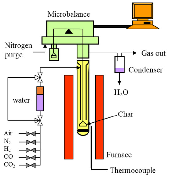
Figure 2. The TGA setup used for gasification, the void arrows and those filled with the grey colour are valves for gas control, the violet and orange colours in the water column mean water and vapour respectively, the yellow colour indicates where quartz reactor is located, the red columns display the location of the furnace, and the green area on top of furnace represents the thermal balance, the violet in the condenser block represents water, and the orange colour on the top-right corner presents a computer.

The total flow of the reacting gas is kept at 25 Ln/h while the gas composition is changed to study the sensitivity of kinetics over the temperature (850, 900, and 950 °C), concentration of gasifying agents (10–40% H₂O and CO₂), and concentration of the gasification products (10–40% H₂ and CO). The experimental conditions are summarized in Table 2 below, and we can see that 105 experiments were made to obtain enough data for kinetics analysis. The steam is generated by bubbling the reacting gas through the saturator containing deionized water at a saturation temperature. The effect of the char amount was studied with 3 mg, 5 mg, and 7 mg. And it is found that the 3 mg is optimal for avoiding external, interparticle, and external diffusions (see the Supplementary Materials). Thus, 3 mg was used throughout the work. The gas flow was maintained at 25 L_n/h to minimize the effect of gas diffusion based on our previous experiences with this TGA setup.

Table 2. Experimental matrix with the TGA apparatus.

Gasification with Steam
	0% H2	10% H2	20% H2	30% H2	40% H2
10% H2O	850,900,950	850,900,950	850,900,950	850,900,950	850,900,950
20% H2O	850,900,950	850,900,950	850,900,950	850,900,950	850,900,950
30% H2O	850,900,950	850,900,950	850,900,950	850,900,950	850,900,950
40% H2O	850,900,950	850,900,950	850,900,950	850,900,950	850,900,950
Gasification with CO2
	0% CO	10% CO	20% CO	30% CO	40% CO
10% CO2	850,900,950	900,950	900,950	900,950	900,950
20% CO2	850,900,950	900,950	850,900,950	900,950	900,950
30% CO2	850,900,950	900,950	900,950	900,950	900,950
40% CO2	850,900,950	900,950	900,950	900,950	900,950

At the beginning, the sample holder is placed outside the furnace and enclosed in N₂ in the tube at room temperature when the furnace is heated up. Once the furnace temperature reaches the set temperature, the furnace is lifted up rapidly to a certain position to heat up the char that is enclosed in the quartz tube in the N₂ flow. Once the mass and temperature are stable, the nitrogen is switched to steam or CO₂ to start the gasification. At the end of the gasification and after another purge with N₂, the gas is changed to air to burn out the possible remaining char. The whole test is completed with another N₂ purge. The air step is used to establish the amount of remaining char in the reactor, and thus can be used to calculate the gasification conversion. Blank tests were also conducted with the empty sample holder and are used to correct the buoyancy effect due to gas change.

3. Data Analysis

3.1. Calculations

The char conversion (X) is calculated with Equation (5) using the initial sample mass (m_i) in N₂ before switching to the gasifying atmosphere and the final mass (m_f) after the last N₂ purge.

$$X={\displaystyle \frac{m_{\mathrm{i}}-m}{m_{\mathrm{i}}-m_{\mathrm{f}}}}$$

(5)

where m is the instantaneous mass during gasification.

The instantaneous rate of char gasification r_inst is the rate based on the amount of residual char present in the holder. We select this method for calculation, because this is a way widely used to calculate the gasification rate and it shows good accuracy. The instantaneous rate is usually used to understand the change in gasification rate and brings important information for the search of suitable kinetics models. Equation (6) below is used to calculate the instantaneous gasification rate.

$$r_{\mathrm{i}\mathrm{n}\mathrm{s}\mathrm{t}}=-{\displaystyle \frac{1}{m}}{\displaystyle \frac{\mathrm{d}m}{\mathrm{d}t}}={\displaystyle \frac{1}{1-X}}{\displaystyle \frac{\mathrm{d}X}{\mathrm{d}t}}$$

(6)

3.2. Uncertainty Analysis

The CI thermobalance equipped with the TGA has a resolution of 0.1 mg, and this means an uncertainty of ±3.3% is expected with the 3 mg used in the experiments. Following a method presented in the previous work [41], the propagation error of the char conversion X and gasification rate r_inst arisen from the uncertainty of the TGA’s mass measurement is estimated to be around ±6.5%. In addition, there could be other uncertainties, e.g., as a result of artificial errors during experiments, experiment repeatability and data fluctuations happen. These were not specifically measured during the experimentation, because the experiment matrix is too big. However, these errors are analyzed and discussed as a whole when we derive the values of the kinetics parameters as seen in Section 4.7 below. With these errors, the accuracy of kinetics data is then analyzed quantitatively, and a confident interval can be defined.

4. Results and Discussion

4.1. Correction of the Mass Change with Blank Tests

Figure 3 presents curves of the original mass (m_original), the corresponding temperature (T_original), a blank test (m_blank), and the corrected mass (m_correct) as a function of time. In the first inert period (inert), there is a big drop of temperature (see the fifth min in the figure). This is because the reactor tube which had a room temperature was positioned inside the furnace and then heated up in a very short time. The temperature then increased quickly to 950 °C; meanwhile, there is a continuous mass loss (see m_original) because of the buoyancy effect. When switching the reacting atmosphere to gasification, we observed a leap of mass both in the original and blank tests. Thus, the buoyancy effect was also captured in the blank test (see m_blank curve), so the blank test allows us to correct the mass signal to m_correct that was finally used as the values of m in Equation (5). After the gasification, there are three times of gas switching (inert, oxidation, and inert). The oxidation was made with air and the data from that period can help us to confirm the value of the final char conversion. In the case of gasification with CO₂, the buoyancy was also checked with blank tests, but the results suggest the buoyancy effect with CO₂ is not relevant. So, we use just the original mass to calculate the char conversion when gasifying with CO₂.

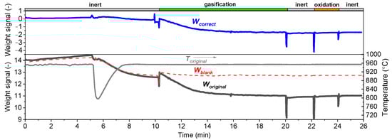
Figure 3. Correction of the original mass (m_original) with a blank test (m_blank) to obtain the correct mass change (m_correct); different reaction stages (inert, gasification, and oxidation) are presented. The original temperature is shown as a function of time. The data was obtained at 950 °C and in a gasification atmosphere of 10% H₂ + 40% H₂O.

4.2. Effect of the Reaction Temperature

Figure 4 below shows the char conversion with 40% H₂O and 40% CO₂ as the gasification medium and without the presence of gasification products (0% H₂ and 0% CO) at 850, 900, and 950 °C. The gasification with steam is slow at 850 °C and becomes faster when the temperature is increased. The char is converted completely at all the three temperatures with 40% H₂O + 0% H₂, although the gasification at 850 °C takes a longer time. In the case with lower steam concentrations (e.g., 10% H₂O), some char was not fully converted due to slower gasification. In the case with CO₂, the conversion is complete at 900 and 950 °C, whereas the conversion is very slow at 850 °C and the conversion is still less than 30% even after 1000 s of gasification. Therefore, in all the experimental conditions, the gasification with H₂O is faster than with CO₂. In all gas concentrations with either H₂O or CO₂ as the gasifying agent, the promotion of the temperature on the gasification is much higher when the temperature is increased from 850 to 900 °C than from 900 °C to 950 °C.

Figure 4. Effect of temperature on the char gasification with (A) 40% H₂O + 0% H₂ and (B) 40% CO₂ + 0% CO.

4.3. Effect of the Concentration of H₂O and CO₂

Figure 5 shows the effect of H₂O and CO₂ concentration on char conversion. It is clearly seen that H₂O concentration has a stronger effect on the gasification rate than CO₂ concentration. For example, an increase in steam concentration from 10% to 20% results in a 50% shorter gasification time (from 700 s to 350 s), leading to a clear increase in gasification rate. The CO₂ gasification curve is less affected by the increase in CO₂ concentration. And when the concentration of CO₂ is 10%, the time for achieving complete conversion is similar to that with 10% H₂O.

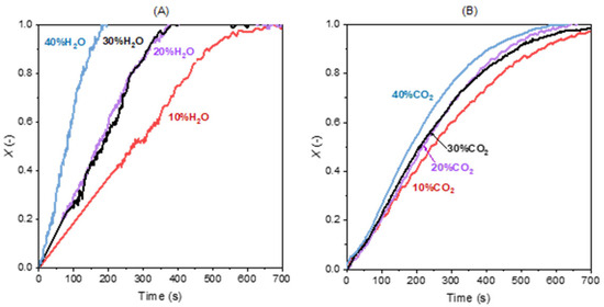
Figure 5. Effect of the concentration of (A) H₂O and (B) CO₂ on gasification without the presence of H₂ and CO (0%) at 900 °C.

In addition, gasification with steam shows a relatively linear X-t curve when the char conversion is lower than around 0.8 and the curve gradually levels off as the conversion approaches one. The gasification with CO₂ has a linear curve below the conversion of 0.3. These linear curves mean that the reaction is not solely controlled by chemical reaction, and the homogeneous model may not be suitable. Therefore, there should be a mixing of several gasification regimes. After the liner segment, the curve shows an “S” shape especially when gasifying with CO₂ and the conversion grows till it gradually levels off. This part of the X-t curves may be described with a homogeneous mechanism and the catalysis may have some mild and irrelevant effect.

4.4. Effect of the Concentration of H₂ and CO

The gasification products CO and H₂ are also inhibitors to the progress of gasification, and the increase in their concentration usually leads to slower gasification, as seen in Figure 6 below. The increase in H₂ from 0 to 40% poses a clear inhibition to gasification and this leads to a continuous and regular decline in the conversion rate. In the case of CO, its inhibition is seen when the CO is increased from 0 to 20%, and the further increase from 20% to 40% does not have a clear inhibition on gasification. The presence of 20–40% CO in 40% CO₂ has a similar gasification rate and time for complete conversion.

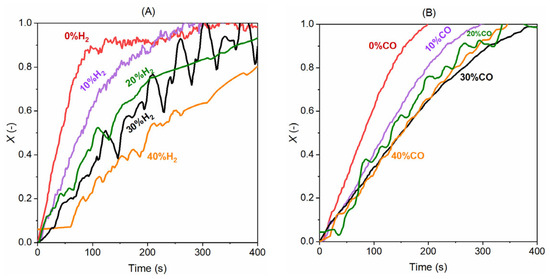
Figure 6. Effect of (A) H₂ concentration with 40% H₂O in steam gasification at 950 °C and (B) CO concentration on the gasification with 40% CO₂ at 950 °C.

4.5. Kinetics Model

Figure 7 displays the instantaneous gasification rate versus the char conversion. In the case of gasification with H₂O, the rate is roughly constant when the conversion is lower than 0.43. After this conversion, the rate increases rapidly to around 0.015 1/s until the conversion reaches 0.8. This new gasification rate is 1.5 times the rate (0.01 1/s) when the conversion is in the range of 0–0.43. Another abrupt increase is also seen at the end of gasification (X = 0.8–1), and this can be attributed to the calculation method (Equation (6)) where the error becomes higher at the end of the conversion, especially when the conversion approaches one. Similar phenomena are, however, not seen with CO₂ gasification. This significant difference in the rate at different stages was also observed in the previous work when gasifying with H₂O in a batch fluidized bed reactor [22] and has been observed with other biomasses in previous works [42,43]. In the case of CO₂ gasification, an increase in gasification is also seen, but the increase is much slower than H₂O gasification. These clearly suggest the gasification cannot be solely described with a homogeneous model, and the second high-rate period can be because of other reasons, like alkali (Na and K) catalysis which is common in biomass gasification. Direct evidence of the alkali’s performance requires in situ/operando studies with microscope, as well as XRD, XPS, and FTIR characterizations, but there are some published works on this with other high-alkali fuels [44,45]. The migration of these metals forms porous skeleton structures and is reported to reach the maximal rate during the middle of reactions [46,47]. Based on the findings of published works, we present below a possible mechanism of the microalgae alkalis migration and their catalysis on gasification. At the beginning of gasification, these alkali components stay in the biomass ash which forms a hollow network. This hollow structure offers a base for carrying the carbon, hydrogen, nitrogen, oxygen, and some organic compounds, and these finally form a porous structure of char [48]. Thus, at the beginning of gasification, the pores are small and the ash cannot be exposed to the gasifying environment; thus, the alkali’s catalysis cannot take effect. But after certain extents of gasification, the pores can be opened greatly, and the alkalis in the network start catalyzing the gasification [49]. Therefore, some gasification with high-alkali fuels showed a faster gasification at the end of the reaction [50], as also observed in the current work.

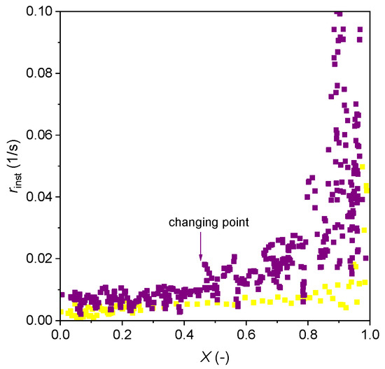
Figure 7. Instantaneous gasification rate change as a function of char conversion with 40% H₂O + 0% H₂ at 850 °C (purple dots) and with 40% CO₂ + 0% CO at 950 °C (yellow dots).

To properly describe the phenomena above, a model which can cover these phenomena and elucidate the mechanisms behind is needed. Such a model is called three-regime model [51] and it considers not only the non-catalytic and catalytic reactions separately but also in a parallel fashion. This model is widely used in biomass gasification [51] and has shown high precision in the modelling of gasification in complex reacting atmosphere. A unique feature of this model is that it does not need structured data and it can be adjusted to single-regime and dual-regime models as needed [51,52]. We present details of the model below and how we adapted the model for use in the current work for kinetics analysis.

The three-regime model is seen in Equation (7), describing the gasification rate (r) as a function of the char conversion. The first regime (r₁) represents a fast gasification with deactivation of catalyst in the catalytic gasification, and the second regime (r₂) corresponds to a first-order gasification without catalysis; the gasification is slower than the first regime. The third regime (r₃) is a faster gasification than the second regime as a result of catalysis of the alkalis in ash.

$$r={\displaystyle \frac{dX}{dt}}=r_1+r_2+r_3$$

(7)

where r₁, r₂, and r₃ take the empirical expressions below:

$$r_1=k_1{\mathrm{e}}^{-\zeta X^2}$$

(8)

$$r_2=k_2(1-X)$$

(9)

$$r_3=k_2(1-X)·{(c·X)}^d$$

(10)

where k₁ and k₂ are the kinetics rates of gasification; ζ, c and d are constants as a function of temperature.

With the rate expression shown in Equation (7), the rate of a gasification can be divided into four categories following a usual method used in the literature [53,54,55]. The combinations are regime 1 + 2 + 3, regime 1 + 2, regime 2 + 3, and regime 2 after comparing between the experimental curve and the model patterns. The current work follows the same method to select the suitable regimes and their combinations of the three-regime model. The four categories of the three-regime model are schematically presented with r_inst versus X in Figure 8. When comparing the model with the experimental curves of the 105 experiments, the initial fast gasification (regime 1) does not happen in any case (see Figure 7 as an example). This means that the first scheme is absent and this is common for the microalgae char. The absence of the first regime has also been observed recently at a bigger scale during the gasification of 2 g microalgae with ZrO₂ in a batch fluidized bed reactor [22]. In addition, a similar phenomenon has been found for the gasification of several biomass chars, and the first regime was proven not relevant [52]. So, the regime 1 + 2 + 3 and regime 1 + 2 are not suitable for the current microalgae char. When comparing the cure of the gasification rate with regime 2 + 3 and regime 2, the regime 2 + 3 agrees well with the phenomenon of a first relatively constant gasification following with a rapid rising of the rate. Therefore, in this work we neglect the first regime and consider just the second and the third regimes (i.e., regime 2 + 3 in Figure 8).

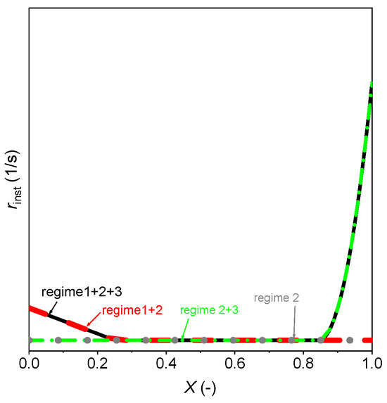
Figure 8. Four types of rate curves with the three-regime model.

Therefore, the three-regime formula in Equation (7) is now reduced to a two-regime model (regime 2 + 3) as seen in Equation (11) below. In addition, Equation (11) also considers the effect of the concentration of the gasification gas and product gas on the constant c (see the last two terms). And the modification of the last two terms proved necessary when fitting the experimental results in this work.

$$r={\displaystyle \frac{dX}{dt}}=k_{2,i}\left(1-X\right)+k_{2,i}\left(1-X\right)·{\left(cX\right)}^d·{p_{gasi}}^n·{p_{prod}}^m$$

(11)

where k₂ is marked with the subscript i to differentiate the types of gasifying agents; when i is H₂O, the gasification is with steam and when i is CO₂, the gasifying agent is CO₂; p_gasi is the partial pressure of the gasifying agent and p_prod is partial pressure of the product gas; n and m denote the exponential constant. For gasification with steam, p_gasi is H₂O and p_prod is H₂, and for gasification with CO₂, p_gasi is CO₂ and p_prod is CO. As seen in Equation (11), k_2,i, c, and d need to be determined to finalize the model.

In addition, the effect of the concentration of gasifying agents and products is included in the calculation of k_2,i. The widely used model of Langmuir–Hinshelwood (L-H) is used for calculation of the rate constant k_2,i, as seen in Equation (12). The L-H model is extensively used in the modelling of coal and biomass gasification and has shown good predictions of the rate constant under complex reaction conditions [56].

$$k_{2,i}={\displaystyle \frac{k_i{p}_{gasi}}{1+K_{gasi}{p}_{gasi}+K_{prod}{p}_{prod}}}$$

(12)

The L-H model can be rewritten to the following formula.

$${\displaystyle \frac{1}{k_{2,i}}}={\displaystyle \frac{1}{k_i{p}_{gasi}}}+{\displaystyle \frac{K_{gasi}}{k_i}}+{\displaystyle \frac{K_{prod}{p}_{prod}}{k_i{p}_{gasi}}}$$

(13)

where the k_i is the reaction rate constant of the gasification; K_gasi and K_prod are the sorption/adsorption constants. The k_i is assumed following the Arrhenius law.

$$k_i={k_{i,0}e}^{-{\displaystyle \frac{E_i}{RT}}}$$

(14)

where k_i,0 is the pre-exponential factor and E_i is the activation energy for the reaction.

The K_gasi, K_prod, c, and d constants are assumed following the Van’t Hoff correlation as seen below. These assumptions are based on previous works [57,58] where more than 10 biomass gasification have been studied, and these equations proved to work well in kinetics analyses.

$$K_{gasi}=K_{gasi,0}{e}^{{\displaystyle \frac{D_{gasi}}{RT}}}$$

(15)

$$K_{prod}=K_{prod,0}{e}^{{\displaystyle \frac{D_{prod}}{RT}}}$$

(16)

$$c=c_0{e}^{{\displaystyle \frac{A_c}{RT}}}$$

(17)

$$d=d_0{e}^{{\displaystyle \frac{A_d}{RT}}}$$

(18)

where K_gasi,0, K_prod,0 c₀, and d₀ are pre-exponential factors, and D_gasi, D_prod, A_c, and A_d are rate constants for the sorption of the gasification agent, the adsorption of product gas, and for the correction of the constants c and d.

4.6. Derivation of Kinetics Parameters

As discussed above, the whole gasification process of the microalgae char is composed by two regimes; a first regime where non-catalyzed gasification dominates and a second regime which is catalyzed by alkalis in the char.

First of all, the k_2,i values were calculated using Equation (6) based on the experimental data and then are used in Equation (11) to derive the kinetics constants. Figure 9 below plots the 1/k_2,H2O versus the 1/p_H2O and 1/k_2,CO2 versus the 1/p_CO2 for the four concentrations of H₂O and CO₂ (10, 20, 30, and 40%) at the three temperatures (850, 900, and 950 °C) when the product gas concentration (H₂ and CO) is set to zero. The plot shows a linear relation between 1/k_2,H2O and 1/p_H2O and 1/k_2,CO2 and 1/p_CO2, and this agrees well with Equation (13) and the linear fitting of these data is used to derive the corresponding kinetics constants. With slopes of these plots, we can obtain the k_H2O and k_CO2 values at the three temperatures; see Equation (13). At the same time, K_H2O and K_CO2 values can be derived with the equation’s intercepts. As seen in Figure 10 later, the k_H2O and k_CO2 are plotted versus the temperature to derive the rate constants and pre-exponential constants through the Arrhenius equation as shown in Equation (14). Meanwhile, K_H2O and K_CO2 are used in Van’t Hoff Equation (15) to calculate the constants K_gasi,0 and D_gasi.

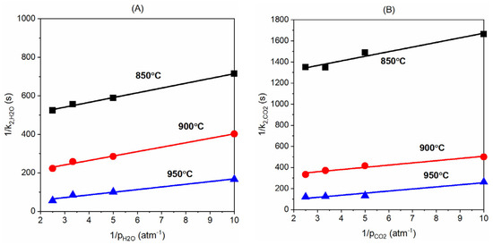
Figure 9. Plots of (A) 1/k_2,H2O versus 1/p_H2O and (B) 1/k_2,CO2 and 1/p_CO2 when the concentration of H₂ and CO is zero, see the L-H model in Equation (13).

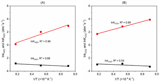
Figure 10. Plots of lnk_i and lnK_gasi versus 1/T for the gasification with (A) H₂O and (B) CO₂; see Equations (14) and (15).

With the k_H2O, k_CO2, K_H2O, and K_CO2 values derived above, we now plot the lnk_i versus 1/T and lnK_gasi versus 1/T plots as seen in Figure 10 below. By applying the Arrhenius law Equation (14) and Van’t Hoff Equation (15), we obtain the k_H2O,0 value (3.99 s⁻¹∙atm⁻¹) from the slope of lnk_H2O and 1/T plots and K_H2O,0 value (3.42 × 10⁻¹⁴ atm⁻¹) from the slope of lnK_H2O versus 1/T plots. The intercepts of the corresponding trend lines are used to derive the values of E_H2O (43.3 kJ/mol) and D_H2O (318.5 kJ/mol). Similarly, we derive the values of k_CO2,0, K_CO2,0, E_CO2, and D_CO2 for the gasification with CO₂ with the slopes and intercepts of the trend lines presented in Figure 10B.

When the parameters (k_i and K_gasi) with regard to the p_H2O and p_CO2 are determined, the kinetics constants (K_prod) with regard to the gasification products (H₂ and CO) can be estimated via Equation (16). Figure 11 shows the plots of lnK_H2 and lnK_CO versus the reciprocal of temperature (1/T). In the case of H₂, we have experimental results at three temperatures (850, 900, and 950 °C), and the lnK_H2 has a linear relation with the temperature (1/T) and the correlation gives a Pearson correlation coefficient of R² = 0.991. In the case of CO, there are only two temperatures that can be used (900 and 950 °C); thus, the lnK_CO has only two data points shown in the figure. This condition is not desirable for the Van’t Hoff correlation, because the uncertainty of the kinetics constants derived with only two temperatures may be higher than the values from three or more temperatures. Despite this, with the constants derived from the two temperatures, the final model can predict the experimental data well as seen later in this work. This means the results from only two temperatures are good and have no significantly high uncertainty. With this information, the K_H2,0, D_H2, K_CO,0, and D_CO are estimated and presented in Table 3 below.

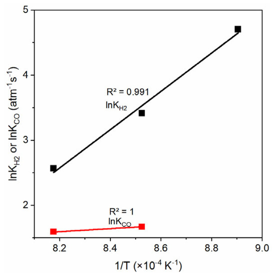
Figure 11. Plots of lnK_H2 and lnK_CO versus the 1/T, see Equation (16).

Figure 12 below displays the effect of the c and d values on the model results. It is clear that a higher value of c leads to a steeper curve, while the effect of the d value depends on the value of c. When c takes one, a higher d value results in a slower gasification, and the opposite is seen when c is higher than one. This pattern helps us to find the proper values of c and d when directly comparing the modelling results with the experimental data, and this in turn helps us to determine the suitable values of c and d. As seen in Figure 12A, when c is set to 2.4 and d is 1.8, the model predicts the experiments well with steam as the gasification gas, and in the case of gasification with CO₂, the c and d values are determined to 2.2 and 1.8; see Figure 12B.

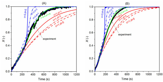
Figure 12. Effect of c and d values on the model’s prediction of experimental results (A) with H₂O as gasifying gas; experimental data from 40% H₂O without H₂ at 850 °C and (B) with CO₂ as gasifying gas; experimental data from 40% CO₂ without CO at 900 °C.

Once the c and d values at different temperatures are found, we apply the Van’t Hoff correlation (Equations (17) and (18)) to determine the values of the pre-exponential factors (c₀ and d₀) and the exponential constants (A_c and A_d). Figure 13 displays the plots of Lnc versus 1/T and Lnd versus 1/T. Using the slopes of the linear trend line in Figure 13, we estimated the values of A_c and A_d, and the intercepts were used to calculate the c₀ and d₀. It is observed that the d values are constant at all the three temperatures, so the A_d is zero for both CO₂ and H₂O.

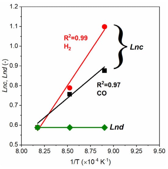
Figure 13. Correlation between Lnc, Lnd, and 1/T for gasification with 40% H₂O and 40% CO₂, without presence of gasification products (H₂ and CO). The Lnd values are the same for H₂ and CO. c.f. Equations (17) and (18).

Then we use the data obtained with the absence of the product in the reacting atmosphere (when p_prod = 0) to find a suitable value of n through in Equation (11) and the plots are shown below in Figure 14. In the case of gasification with H₂O, when n is four, the model fits the experimental data well. When n is smaller than four, the model returns values higher than the experimental results, and a lower value is returned when a bigger n is used. The similar trend is also seen for CO₂ gasification as seen in Figure 14B. The model with n = 0.2 and 0.3 predicts the first part of the gasification well but overpredicts the experimental results slightly when conversion is higher than 0.6. In contrast, when n is set to 0.4, the model predicts the experimental results better at higher conversions. Therefore, we select 0.4 as the value of n for CO₂ gasification. Following the same process, we determined the value of m for the gasification model.

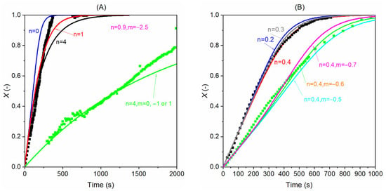
Figure 14. Determination of the model’s n and m values by fitting the model results and experimental results; (A) gasification with steam (black dots: 20% H₂O + 0% H₂; green dots: 10% H₂O + 20% H₂); (B) gasification with CO₂ (black dots: 30% CO₂ + 0% CO; green dots: 10% CO₂ + 10% CO). The lines are modelling results with different n/m pairs at 900 °C.

Table 3 below summarizes the values of different kinetics parameters and constants. The activation energy for gasification with steam is 43.3 kJ/mol and this is much lower than the value with CO₂ (91.6 kJ/mol). This aligns well with the phenomenon that the gasification with H₂O is faster than the gasification with CO₂. The activation energy of gasification with steam is lower than the apparent activation energy (49 kJ/mol) reported in An et al. [59], where in addition to using a microalga, a hematite was also used to supply oxygen for the gasification. Although the reacting atmosphere is different as compared to the current work and the hematite can enhance the gasification, it can be seen that the intrinsic kinetics is faster than the apparent kinetics. In a similar reacting condition, Wu et al. [60] reported an activation energy of 180–380 kJ/mol for a Chlorella microalga gasification with Fe₂O₃ as an oxygen carrier without the presence of H₂O or a CO₂ gasifiying agent in the reacting atmosphere. Bach et al. [26] studied the kinetics of a slow char gasification with CO₂ and an activation energy of 300–360kJ/mol was reported. This activation energy is also much higher than what we have obtained in the current work with CO₂. This shows that the fast char is much easier for gasification than the slow char. The D_H2O value (318.5 kJ/mol) is much higher than the D_CO2 value (187.4 kJ/mol), and this suggests that the H₂O has a better sorption than CO₂. This again supports the phenomenon that H₂O has a faster gasification than CO₂. Looking at the D_H2 and D_CO values, we can clearly see the value for H₂ is positive whereas the value for CO is negative. And as seen in Figure 11 above, the LnK_H2 is higher than LnK_CO in the studied temperature range; this means the H₂ has a slower adsorption from the char surface as compared to CO; thus, the former has a stronger inhibition on gasification. This may explain the usually observed stronger H₂ inhibition on the gasification than CO [61].

Table 3. Kinetics parameters obtained for fast microalgae char gasification.

	Steam		CO2
kH2O,0 (s−1∙atm−1)	3.99	kCO2,0 (s−1∙atm−1)	460
EH2O (kJ/mol)	43.3	ECO2 (kJ/mol)	91.6
KH2O,0 (atm−1)	3.42 × 10−14	KCO2,0 (atm−1)	5.67 × 10−8
DH2O (kJ/mol)	318.5	DCO2 (kJ/mol)	187.4
KH2,0 (atm−1)	4.23×10−10	KCO,0 (atm−1)	315
DH2 (kJ/mol)	244.9	DCO (kJ/mol)	−42.1
c0 (atm−1)	7.42 × 10−2	c0 (atm−1)	5.6 × 10−3
Ac (kJ/mol)	32.7	Ac (kJ/mol)	58.5
d0	1.8	d0	1.8
Ad	0	Ad	0
n	4	n	0.4
m	0	m	−0.6

Table 3. Kinetics parameters obtained for fast microalgae char gasification.

	Steam		CO2
kH2O,0 (s−1∙atm−1)	3.99	kCO2,0 (s−1∙atm−1)	460
EH2O (kJ/mol)	43.3	ECO2 (kJ/mol)	91.6
KH2O,0 (atm−1)	3.42 × 10−14	KCO2,0 (atm−1)	5.67 × 10−8
DH2O (kJ/mol)	318.5	DCO2 (kJ/mol)	187.4
KH2,0 (atm−1)	4.23×10−10	KCO,0 (atm−1)	315
DH2 (kJ/mol)	244.9	DCO (kJ/mol)	−42.1
c0 (atm−1)	7.42 × 10−2	c0 (atm−1)	5.6 × 10−3
Ac (kJ/mol)	32.7	Ac (kJ/mol)	58.5
d0	1.8	d0	1.8
Ad	0	Ad	0
n	4	n	0.4
m	0	m	−0.6

4.7. Evaluation of the Model

Figure 15 below displays that the model predicts the steam gasification better at a higher temperature. At temperatures of 850 and 900 °C, the conversion curve below X = 0.4 can be well-captured by the model, while above this conversion, the model returns a lower value as compared to the experiments. Particularly, when the temperature is 850 °C, there is a speed-up trend as the conversion goes higher than 0.4, and this is not fully captured by the model. But the experiments at 900 and 950 °C are well-predicted with the model. Figure 15B,C compares the model predictions and experiments under various reacting conditions. It can be seen that the model gives satisfactory predictions for steam gasification of the fast microalgae char in a complex reacting atmosphere.

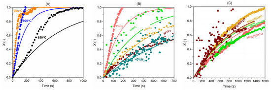
Figure 15. Comparison of the carbon conversion (X) between experiments (dots) and model (lines): (A) 40% H₂O + 0% H₂ at 850, 900, and 950 °C; (B) 40% H₂O with five H₂ concentrations (0, 10, 20, 30, 40%) at 900 °C and (C) H₂:H₂O = 1:1 (10% H₂ + 10% H₂O, 20% H₂ + 20% H₂O, 30% H₂ + 30% H₂O and 40% H₂ + 40% H₂O) at 900 °C.

In the case of CO₂ gasification, again at higher temperatures, the model predicts better, and at 850 °C, the model captures the initial conversions well but cannot bring accurate predictions for the remaining conversion; see Figure 16. With presence of CO in the gasifying atmosphere, the model predicts the experimental data well and captures the effect of CO’s inhibition well; see Figure 16B. In Figure 16C, the model results are compared with the experiments under conditions with a CO₂-to-CO ratio of 1:1. It is seen that the model predicts the data very well with 40% CO + 40% CO₂ or 20% CO + 20% CO₂ in the gasification mixture, but returns underestimations for the gasification with 10% CO + 10% CO₂ and 30% CO + 30% CO₂. The discrepancy is considered a result of uncertainties from the experiments. But overall, the model can estimate the experimental results of the gasification with CO₂ well.

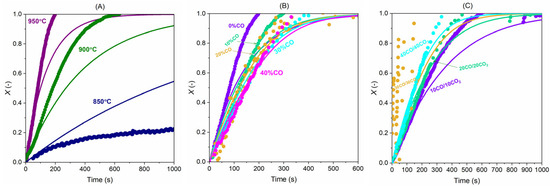
Figure 16. Comparison of the carbon conversion (X) between experiments (dots) and model (lines): (A) 40%CO₂ + 0%CO at 850, 900, and 950 °C; (B) 40%CO₂ with five CO concentrations (0, 10, 20, 30, 40%) at 950 °C and (C) CO:CO₂ = 1:1 (10% CO + 10% CO₂, 20% CO + 20% CO₂, 30% CO + 30% CO₂ and 40% CO + 40% CO₂) at 950 °C.

Figure 17 further displays the overall confidence interval of the model when compared with the experimental results. As discussed above, this uncertainty may come from TGA’s measurement (±3.3%), artificial error, and data fluctuation. The overall uncertainty shown in this figure considers all these factors. It can be seen that the model predicts almost all the experimental data when the error is within ±25% for gasification with H₂O and CO₂. Around 1/3 of the data can be well-captured by the model within an error of ±10%, and there are also several data beyond the ±25% interval. Overall, the model has a good capability in predicting the experimental results, and when applied, a confidence interval of ±25% should be noticed.

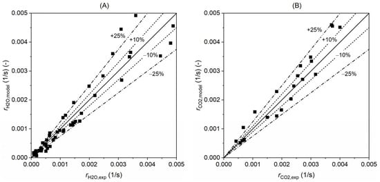
Figure 17. Confidence interval of the kinetics model for the gasification with (A) H₂O and (B) CO₂. The x-axis shows the value of gasification rate from the experiments and y-axis is the model results. The lines represent the interval of confidence with error of ±10% and ±25%.

4.8. Implication to CLG Application

The intrinsic kinetics model can be implemented in a complete reactor model, process model, and CFD model for not only a CLG but also CLC (chemical looping combustion) process which also involves char gasification. It can also be used to calculate key parameters for use in system design and operation, for example, the char residence time in the fuel reactor. Figure 18 below presents the time needed for reaching a char conversion of X = 0.99 with H₂O and CO₂ as gasifying agents. Obviously, when the concentration of gasifying agent is higher, the time needed is shorter. And the inhibition by H₂ and CO is also clearly seen; a longer gasification time is needed when the concentration of H₂ and CO becomes higher. The contour can be used to estimate the residence time of char in the fuel reactor of a CLG system. For example, if we use 70% steam as gasifying gas in the fuel reactor, the outlet gas can contain around 15% H₂, 8% CO, and 7% CO₂ based on our experience in the operation of continuous CLG units. In this case, a char residence time of around 5 min can ensure a complete char conversion; see Figure 18A. In this condition, the gasification with CO₂ is not relevant because its concentration is low (7%) and needs a longer char residence time (around 10 min), as seen in Figure 18B. Notably, the contour presented in Figure 18 does not consider the presence of the toxygen carrier, and thus the time shown here is expected to be longer than real CLG process. In the real CLG process, the gasification will become faster because the oxygen carrier can react with H₂ and CO, removing the inhibition and accelerating the gasification. How fast the gasification can be will depend on the type of oxygen carrier.

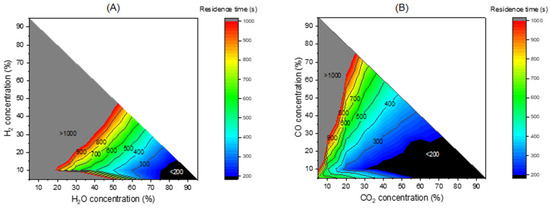
Figure 18. Contour of residence time in seconds for reaching a conversion of X = 0.99 of the fast char gasification at 950 °C (A) with H₂O and (B) with CO₂ as the gasification agents considering the inhibition of H₂ and CO.

5. Conclusions

Intrinsic gasification kinetics of a fast microalgae char is studied with steam and CO₂ in a TGA apparatus covering a wide range of reacting atmosphere for the CLG process. A modified two-regime kinetics model is employed for kinetics analysis. The Langmuir–Hinshelwood model is used to describe the rate constant, considering the inhibition of gasification products (H₂ and CO). The model has a first relatively constant gasification and a second catalytic accelerating gasification and was found fitting the experiments well, with both H₂O and CO₂ as the gasifying agents. The values of kinetics parameters are derived. The activation energy E_H2O and sorption and desorption constants D_H2O and D_H2 during steam gasification are 43.3, 318.5, and 244.9 kJ/mol, and the corresponding pre-exponential factors k_H2O,0, K_H2O,0, and K_H2,0 are 3.99 s⁻¹∙atm⁻¹, 3.42 × 10⁻¹⁴ atm⁻¹, and 4.23 × 10⁻¹⁰ atm⁻¹. For the gasification with CO₂, the activation energy E_CO2 and the constants D_CO2 and D_CO are 91.6, 187.4, and −42.1 kJ/mol, and the pre-exponential factors k_CO2,0, K_CO2,0, and K_CO,0 are 460, 5.67 × 10⁻⁸, and 315 atm⁻¹. The model predicts the experimental results well and is proved having an overall uncertainty of ±25%, and can be used for the Spirulina microalga in the temperature range of 850–950 °C. Based on the model, a contour of char residence time is mapped, and this is useful for reactor design and optimization. In addition, to be applicable in the CLG process, the model can also be used in other gasification/combustion processes where H₂O or CO₂ is used as a gasifying agent. Future work will focus on how to implement the kinetics in different reactor models.

References

- Zhao, X.; Zhou, H.; Sikarwar, V.S.; Zhao, M.; Park, A.-H.A.; Fennell, P.S.; Shen, L.; Fan, L.-S. Biomass-based chemical looping technologies: The good, the bad and the future. Energy Environ. Sci. 2017, 10, 1885–1910. [Google Scholar] [CrossRef]
- Mattisson, T.; Keller, M.; Linderholm, C.; Moldenhauer, P.; Rydén, M.; Leion, H.; Lyngfelt, A. Chemical-looping technologies using circulating fluidized bed systems: Status of development. Fuel Process. Technol. 2018, 172, 1–12. [Google Scholar] [CrossRef]
- Goel, A.; Moghaddam, E.M.; Liu, W.; He, C.; Konttinen, J. Biomass chemical looping gasification for high-quality syngas: A critical review and technological outlooks. Energy Convers. Manag. 2022, 268, 116020. [Google Scholar] [CrossRef]
- El-Nagar, R.A.; Ghanem, A.A. Syngas production, properties, and its importance. In Sustainable Alternative Syngas Fuel; Ghenai, C., Inayat, A., Eds.; IntechOpen: London, UK, 2019. [Google Scholar]
- Konarova, M.; Aslam, W.; Perkins, G. Chapter 3—Fischer-Tropsch synthesis to hydrocarbon biofuels: Present status and challenges involved. In Hydrocarbon Biorefinery; Maity, S.K., Gayen, K., Bhowmick, T.K., Eds.; Elsevier: London, UK, 2022; pp. 77–96. [Google Scholar]
- Angelico, R.; Giametta, F.; Bianchi, B.; Catalano, P. Green Hydrogen for Energy Transition: A Critical Perspective. Energies 2025, 18, 404. [Google Scholar] [CrossRef]
- Samprón, I.; de Diego, L.F.; García-Labiano, F.; Izquierdo, M.T. Optimization of synthesis gas production in the biomass chemical looping gasification process operating under auto-thermal conditions. Energy 2021, 226, 120317. [Google Scholar] [CrossRef]
- Dieringer, P.; Marx, F.; Michel, B.; Ströhle, J.; Epple, B. Design and control concept of a 1 MWth chemical looping gasifier allowing for efficient autothermal syngas production. Int. J. Greenh. Gas Control 2023, 127, 103929. [Google Scholar] [CrossRef]
- Daneshmand-Jahromi, S.; Sedghkerdar, M.H.; Mahinpey, N. A review of chemical looping combustion technology: Fundamentals, and development of natural, industrial waste, and synthetic oxygen carriers. Fuel 2023, 341, 127626. [Google Scholar] [CrossRef]
- Mishra, S.; Upadhyay, R.K. Review on biomass gasification: Gasifiers, gasifying mediums, and operational parameters. Mater. Sci. Energy Technol. 2021, 4, 329–340. [Google Scholar] [CrossRef]
- Mendiara, T.; García-Labiano, F.; Abad, A.; Gayán, P.; de Diego, L.F.; Izquierdo, M.T.; Adánez, J. Negative CO2 emissions through the use of biofuels in chemical looping technology: A review. Appl. Energy 2018, 232, 657–684. [Google Scholar] [CrossRef]
- IEA. Technology Roadmap—Biofuels for Transport; IEA: Paris, France, 2011. [Google Scholar]
- Forján, E.; Navarro, F.; Cuaresma, M.; Vaquero, I.; Ruíz-Domínguez, M.C.; Gojkovic, Ž.; Vázquez, M.; Márquez, M.; Mogedas, B.; Bermejo, E.; et al. Microalgae: Fast-Growth Sustainable Green Factories. Crit. Rev. Environ. Sci. Technol. 2015, 45, 1705–1755. [Google Scholar] [CrossRef]
- Leong, Y.K.; Chang, J.-S. Microalgae-based biochar production and applications: A comprehensive review. Bioresour. Technol. 2023, 389, 129782. [Google Scholar] [CrossRef] [PubMed]
- Chiaramonti, D.; Prussi, M.; Buffi, M.; Casini, D.; Rizzo, A.M. Thermochemical conversion of microalgae: Challenges and opportunities. Energy Procedia 2015, 75, 819–826. [Google Scholar] [CrossRef]
- Lyngfelt, A.; Leckner, B. A 1000MWth boiler for chemical-looping combustion of solid fuels—Discussion of design and costs. Appl. Energy 2015, 157, 475–487. [Google Scholar] [CrossRef]
- Liu, Y.; Yin, K.; Wu, J.; Mei, D.; Konttinen, J.; Joronen, T.; Hu, Z.; He, C. Ash chemistry in chemical looping process for biomass valorization: A review. Chem. Eng. J. 2023, 478, 147429. [Google Scholar] [CrossRef]
- Lin, Y.; Wang, H.; Wang, Y.; Huo, R.; Huang, Z.; Liu, M.; Wei, G.; Zhao, Z.; Li, H.; Fang, Y. Review of Biomass Chemical Looping Gasification in China. Energy Fuels 2020, 34, 7847–7862. [Google Scholar] [CrossRef]
- Liu, G.; Liao, Y.; Wu, Y.; Ma, X.; Chen, L. Characteristics of microalgae gasification through chemical looping in the presence of steam. Int. J. Hydrogen Energy 2017, 42, 22730–22742. [Google Scholar] [CrossRef]
- Liu, G.; Liao, Y.; Wu, Y.; Ma, X. Evaluation of Sr-substituted Ca2Fe2O5 as oxygen carrier in microalgae chemical looping gasification. Fuel Process. Technol. 2019, 191, 93–103. [Google Scholar] [CrossRef]
- Wang, Y.; Xing, Y.; Hong, C. Chemical looping gasification of microalgae biomass with Fe-based oxygen carrier for gas production and kinetic behavior. Chem. Eng. Process.-Process Intensif. 2025, 210, 110215. [Google Scholar] [CrossRef]
- Mei, D.; García-Labiano, F.; Abad, A.; Adanez-Rubio, I.; Mattisson, T. Evaluation of ilmenite, manganese ore, LD slag and iron sand oxygen carriers for chemical looping gasification with microalgae. Fuel Process. Technol. 2025, 275, 108266. [Google Scholar] [CrossRef]
- Su, M.; Zhao, H.; Tian, X.; Zhang, P.; Du, B.; Liu, Z. Intrinsic reduction kinetics investigation on a hematite oxygen carrier by CO in chemical looping combustion. Energy Fuels 2017, 31, 3010–3018. [Google Scholar] [CrossRef]
- Samiee-Zafarghandi, R.; Azari, A. Kinetics Modeling of Marine Microalgal Biomass in Non-Catalytic Supercritical Water Gasification for Hydrogen and Methane Production. Environ. Energy Econ. Res. 2025, 9, S107. [Google Scholar]
- Ji, G.; Raheem, A.; Wang, X.; Fu, W.; Qu, B.; Gao, Y.; Li, A.; Zhao, M.; Dong, W.; Zhang, Z. Kinetic Analysis of Algae Gasification by Distributed Activation Energy Model. Processes 2020, 8, 927. [Google Scholar] [CrossRef]
- Bach, Q.-V.; Chen, W.-H.; Sheen, H.-K.; Chang, J.-S. Gasification kinetics of raw and wet-torrefied microalgae Chlorella vulgaris ESP-31 in carbon dioxide. Bioresour. Technol. 2017, 244, 1393–1399. [Google Scholar] [CrossRef] [PubMed]
- Burgert, B.; Hattingh, R.C.; Everson, H.W.J.P.; Neomagus, J.R.B. Assessing the catalytic effect of coal ash constituents on the CO2 gasification rate of high ash, South African coal. Fuel Process. Technol. 2011, 92, 2048–2054. [Google Scholar] [CrossRef]
- Neelam, K.; Sujan, S.; Gajanan, S.; Vishal, C.; Rupak, R.; Sudipta, D.; Prakash, D.C. Comparison of CO2 gasification reactivity and kinetics: Petcoke, biomass and high ash coal. Biomass Convers. Biorefinery 2022, 12, 2277–2290. [Google Scholar]
- González-Vázquez, M.P.; García, R.; Gil, M.V.; Pevida, C.; Rubiera, F. Unconventional biomass fuels for steam gasification: Kinetic analysis and effect of ash composition on reactivity. Energy 2018, 155, 426–437. [Google Scholar] [CrossRef]
- González-Vázquez, M.P.; García, R.; Gil, M.V.; Pevida, C.; Rubiera, F. Comparison of the gasification performance of multiple biomass types in a bubbling fluidized bed. Energy Convers. Manag. 2018, 176, 309–323. [Google Scholar] [CrossRef]
- Dupont, C.; Jacob, S.; Marrakchy, K.O.; Hognon, C.; Grateau, M.; Labalette, F.; Da Silva Perez, D. How inorganic elements of biomass influence char steam gasification kinetics. Energy 2016, 109, 430–435. [Google Scholar] [CrossRef]
- González, W.A.; Nilsson, S.; Fuentes-Cano, D.; Ronda, A.; Gómez-Barea, A. Steam Gasification Reactivity of Potassium-Doped Wood Chars in a Fluidized Bed. Energy Fuels 2025, 39, 20621–20634. [Google Scholar] [CrossRef]
- Mei, J.; Quan, S.; Yang, H.; Zhang, M.; Zhou, T.; Yang, X.; Zhang, M.; Mun, T.-Y.; Li, Z.; Kim, R.-G. Research Progress and Perspectives of the Reaction Kinetics of Fe-Based Oxygen Carriers in Chemical Looping Combustion. Energies 2025, 18, 2313. [Google Scholar] [CrossRef]
- Nowak, B.; Karlström, O.; Backman, P.; Brink, A.; Zevenhoven, M.; Voglsam, S.; Winter, F.; Hupa, M. Mass transfer limitation in thermogravimetry of biomass gasification. J. Therm. Anal. Calorim. 2013, 111, 183–192. [Google Scholar] [CrossRef]
- De Wilde, J. Measuring the intrinsic kinetics of heterogeneously catalyzed reactions in gas–solid bubbling fluidized beds: Criteria and case study. Chem. Eng. J. 2025, 517, 164030. [Google Scholar] [CrossRef]
- Lobo, L.S. Intrinsic kinetics in carbon gasification: Understanding linearity, “nanoworms” and alloy catalysts. Appl. Catal. B 2014, 148, 136–143. [Google Scholar] [CrossRef]
- Zheng, C.; Su, M.; Zhao, H. The intrinsic kinetic study on oxidation of a Cu-based oxygen carrier in chemical looping combustion. Fuel 2023, 334, 126720. [Google Scholar] [CrossRef]
- Chen, C.; Wang, J.; Liu, W.; Zhang, S.; Yin, J.; Luo, G.; Yao, H. Effect of pyrolysis conditions on the char gasification with mixtures of CO2 and H2O. Proc. Combust. Inst. 2013, 34, 2453–2460. [Google Scholar] [CrossRef]
- Yaqub, Z.T.; Oboirien, B.O. Process Modelling of Chemical Looping Combustion of Paper, Plastics, Paper/Plastic Blend Waste, and Coal. ACS Omega 2020, 5, 22420–22429. [Google Scholar] [CrossRef]
- Niu, Y.; Chi, Z.; Li, M.; Du, J.; Han, F. Advancements in biomass gasification and catalytic tar-cracking technologies. Mater. Rep. Energy 2024, 4, 100295. [Google Scholar] [CrossRef]
- Mei, D.; Linderholm, C.; Lyngfelt, A. Performance of an oxy-polishing step in the 100 kWth chemical looping combustion prototype. Chem. Eng. J. 2021, 409, 128202. [Google Scholar] [CrossRef]
- Hashimoto, K.; Miura, K.; Xu, J.-J.; Watanabe, A.; Masukami, H. Relation between the gasification rate of carbons supporting alkali metal salts and the amount of oxygen trapped by the metal. Fuel 1986, 65, 489–494. [Google Scholar] [CrossRef]
- Kramb, J.; Konttinen, J.; Gómez-Barea, A.; Moilanen, A.; Umeki, K. Modeling biomass char gasification kinetics for improving prediction of carbon conversion in a fluidized bed gasifier. Fuel 2014, 132, 107–115. [Google Scholar] [CrossRef]
- Mei, Y.-G.; Wang, Z.-Q.; Zhang, H.; Zhang, S.-J.; Fang, Y.-T. In-situ study of effect of migrating alkali metals on gasification reactivity of coal char. J. Fuel Chem. Technol. 2021, 49, 735–741. [Google Scholar] [CrossRef]
- Dayton, D.C.; French, R.J.; Milne, T.A. Direct Observation of Alkali Vapor Release during Biomass Combustion and Gasification. 1. Application of Molecular Beam/Mass Spectrometry to Switchgrass Combustion. Energy Fuels 1995, 9, 855–865. [Google Scholar] [CrossRef]
- Zhang, H.; Shen, Z.; Liang, Q.; Liu, H. Mechanism and interaction of alkaline-earth metal migration induced ash transformation and carbon structure evolution for single coal particle high-temperature gasification. Chem. Eng. J. 2024, 495, 153575. [Google Scholar] [CrossRef]
- Jiao, Y.; Tian, L.; Yu, S.; Song, X.; Wu, Z.; Wei, J.; Xu, J. AAEM Species Migration/Transformation during Co-Combustion of Carbonaceous Feedstocks and Synergy Behavior on Co-Combustion Reactivity: A Critical Review. Energies 2023, 16, 7473. [Google Scholar] [CrossRef]
- Matsuoka, K.; Akiho, H.; Xu, W.-C.; Gupta, R.; Wall, T.F.; Tomita, A. The physical character of coal char formed during rapid pyrolysis at high pressure. Fuel 2005, 84, 63–69. [Google Scholar] [CrossRef]
- Korus, A.; Jagiello, J.; Jaroszek, H.; Copik, P.; Szlęk, A. Variation of pore development scenarios by changing gasification atmosphere and temperature. Energy 2024, 289, 129897. [Google Scholar] [CrossRef]
- Lahijani, P.; Zainal, Z.A.; Mohamed, A.R.; Mohammadi, M. CO2 gasification reactivity of biomass char: Catalytic influence of alkali, alkaline earth and transition metal salts. Bioresour. Technol. 2013, 144, 288–295. [Google Scholar] [CrossRef]
- Umeki, K.; Moilanen, A.; Gómez-Barea, A.; Konttinen, J. A model of biomass char gasification describing the change in catalytic activity of ash. Chem. Eng. J. 2012, 207, 616–624. [Google Scholar] [CrossRef]
- Abad, A.; Condori, O.; de Diego, L.F.; García-Labiano, F. Determining intrinsic biomass gasification kinetics and its application on gasification of pelletized biomass: Simplifying the process for use in chemical looping processes. Fire 2026, 9, 9. [Google Scholar] [CrossRef]
- Grasa, G.; Martínez, I.; Murillo, R. Gasification kinetics of chars from diverse residues under suitable conditions for the Sorption Enhanced Gasification process. Biomass Bioenergy 2024, 180, 107000. [Google Scholar] [CrossRef]
- Tao, J.; Shi, Z.; Liu, Y.; Jia, Y.; Wang, Z.; Wang, X.; Chen, Y.; Yu, B.; Xu, S.; Xu, D.; et al. Study on intrinsic reaction kinetics of coal char gasification based on general surface activation function model. Fuel 2025, 395, 135188. [Google Scholar] [CrossRef]
- Xue, J.; Dong, Z.; Chen, H.; Zhang, M.; Zhao, Y.; Chen, Y.; Chen, S. Gasification of the Char Residues with High Ash Content by Carbon Dioxide. Energies 2024, 17, 4432. [Google Scholar] [CrossRef]
- Irfan, M.F.; Usman, M.R.; Kusakabe, K. Coal gasification in CO2 atmosphere and its kinetics since 1948: A brief review. Energy 2011, 36, 12–40. [Google Scholar] [CrossRef]
- Tellinghuisen, J. Van’t Hoff analysis of K° (T): How good…or bad? Biophys. Chem. 2006, 120, 114–120. [Google Scholar] [CrossRef] [PubMed]
- Purnomo, V.; Staničić, I.; Mei, D.; Soleimanisalim, A.H.; Mattisson, T.; Rydén, M.; Leion, H. Performance of iron sand as an oxygen carrier at high reduction degrees and its potential use for chemical looping gasification. Fuel 2023, 339, 127310. [Google Scholar] [CrossRef]
- An, F.; Shao, D.; Gai, D.; Yu, Y.; Zhong, Z.; Wang, X. Activity and kinetic characterization of coal and microalgae chemical looping co-gasification based on thermogravimetric analysis. Thermochim. Acta 2025, 750, 180052. [Google Scholar] [CrossRef]
- Wu, S.; Zhang, B.; Yang, B.; Shang, J.; Zhang, H.; Guo, W.; Wu, Z. Chemical looping gasification characteristics and kinetic analysis of Chlorella and its organic components. Carbon Resour. Convers. 2022, 5, 211–221. [Google Scholar] [CrossRef]
- Zhang, R.; Wang, Q.H.; Luo, Z.Y.; Fang, M.X.; Cen, K.F. Coal Char Gasification in the Mixture of H2O, CO2, H2, and CO under Pressured Conditions. Energy Fuels 2014, 28, 832–839. [Google Scholar] [CrossRef]
Disclaimer/Publisher’s Note: The statements, opinions and data contained in all publications are solely those of the individual author(s) and contributor(s) and not of MDPI and/or the editor(s). MDPI and/or the editor(s) disclaim responsibility for any injury to people or property resulting from any ideas, methods, instructions or products referred to in the content. |
© 2026 by the authors. Licensee MDPI, Basel, Switzerland. This article is an open access article distributed under the terms and conditions of the Creative Commons Attribution (CC BY) license.