Abstract
Accurate photovoltaic (PV) power forecasting is critical for the stable operation of power systems. Existing methods rely solely on historical data, which significantly decline in forecasting accuracy at 3–4 h ahead. To address this problem, a novel ultra-short-term PV power forecasting method based on temporal attention-variable parallel fusion encoder network is proposed to enhance the stability of forecasting results by incorporating Numerical Weather Prediction data to correct temporal predictions. Specifically, independent encoding modules are constructed for both historical power sequences and future NWP sequences, enabling deep feature extraction of their respective temporal characteristics. During the decoding phase, a two-stage coupled decoding strategy is employed: for 1–8 steps predictions, the model relies solely on temporal features, while for 9–16 steps horizons, it dynamically fuses encoded information from historical power data and future NWP inputs. This approach allows for accurate characterization of future trend dynamics. Experimental results demonstrate that, compared with conventional methods, the proposed model reduces the average normalized root mean square error (NRMSE) at 4th ultra-short-term forecasting by 0.50–5.20%, while it improves the by 0.047–0.362, validating the effectiveness of the proposed approach.
1. Introduction
With the progressive depletion of fossil fuels and the growing energy gap, countries around the world have successively proposed carbon neutrality targets and accelerated the development of multi-energy power systems centered on renewable energy sources [1,2]. However, the increase in renewables in power systems, primarily wind and solar, due to the randomness and volatility of wind and PV output, results in the increasingly prominent impact of renewable energy on the stability of the power system. Accurate power forecasting plays a crucial role in enabling grid operators to schedule reserve capacity in advance, thereby mitigating the impact of large-scale renewable integration on the grid. It serves as a key enabling technology for promoting the effective utilization of renewable energy [3].
Ultra-short-term power forecasting (USTPF), which aims to predict power output within a 15 min–4 h horizon, is currently one of the most extensively studied and technically mature forecasting approaches. It serves as a key reference for intra-day grid dispatch decisions. Due to the short forecasting window and high execution frequency, statistical methods, especially time series-based machine learning methods, owing to their fast response, efficient data utilization, and flexible modeling capabilities, have become mainstream in ultra-short-term (UST) forecasting. From the developmental perspective, USTPF techniques can be broadly categorized into two stages [4,5]:
(1) Algorithm-centric development stage. This phase emphasizes the use of more powerful regression algorithms and optimization techniques to enhance model performance. Representative approaches include neural network algorithms [6,7,8,9] (e.g., back propagation neural networks (BPNNs), dynamic neural networks (DNNs)), kernel-based learning algorithms [10,11,12,13] (e.g., support vector machines (SVMs), relevance vector machines (RVMs), extreme learning machines (ELMs), Gaussian processes (GPs)), and deep learning algorithms [14,15,16,17] (e.g., recurrent neural networks (RNNs), convolutional neural networks (CNNs), denoising autoencoders (DAs), deep belief networks (DBNs)). Ref. [18] proposed a hybrid forecasting model combining genetic algorithms and a BPNN; by performing autocorrelation analysis, the model identifies the most influential historical wind speed, uses wind speed, temperature, humidity, and air pressure as input variables, and genetic algorithms are employed to optimize the initial weights and thresholds of the BPNN, which is then used to construct 1 h, 2 h, and 3 h forecasting models. In [19], an Autoregressive Integrated Moving Average Model (ARIMA) model with stochastic coefficients was developed to account for the impact of cloud cover, atmospheric turbidity, and precipitation on PV generation. Ref. [20] introduced a Vision Transformer-based model for PV power forecasting, which utilizes both target and surrounding PV sensor data. By leveraging spatial information and auxiliary sensor inputs, the model can anticipate cloud movement, thereby improving USTPF accuracy. Ref. [21] conducted a systematic benchmark of five Transformer variants (Autoformer, Informer, FEDformer, DLinear, and PatchTST), and incorporated Adaptive Conformal Inference (ACI) to quantify uncertainty in real time. Results showed that PatchTST, with its patch-based temporal tokenization, achieved superior accuracy for 1 h ahead PV power forecasting. While advanced forecasting and optimization algorithms have significantly improved prediction accuracy, static and independent models still struggle to adapt to the high randomness of weather systems and seasonal variability.
(2) Fine-grained modeling development stage. To enhance model adaptability, recent research has focused on more refined forecasting strategies, such as clustering training samples based on weather conditions [22,23,24,25], thereby improving the model’s responsiveness to the current weather scenario. For sites with pronounced seasonal characteristics, models can be tailored by month or season, or different algorithms can be applied accordingly. In Ref. [26], site data were grouped by season and weather type (sunny, cloudy, rainy), and a hybrid artificial neural network (ANN) model optimized using Gray Wolf Optimization (GWO) and Genetic Algorithms (GAs) was employed. By tuning the number of hidden layers and neurons, the model improved PV forecasting performance under varying weather conditions. In Ref. [27], clustering algorithms were used to classify historical PV data into distinct scenarios, followed by modeling with a multivariate evolving fuzzy time series algorithm, achieving high-precision forecasting across multiple scenarios.
On the other hand, some researchers have explored the joint modeling method [2], which integrates resource and power information from homogeneous or heterogeneous power stations into a single model. By incorporating input data from multiple sites and time periods, these models can capture more comprehensive temporal and spatial information. Numerous studies have demonstrated that joint modeling significantly enhances forecasting accuracy for every target. For instance, Ref. [28] proposed a joint forecasting model based on the spatiotemporal attention network, which captures the spatial and temporal correlations of regional wind and solar resources, thereby improving the forecasting accuracy for eight wind farms and six PV stations within the region. In [29], a regional wind–solar joint forecasting model was developed using the Time Pattern Attention LSTM (TPA-LSTM) algorithm; by introducing an improved loss function, the model effectively shares correlated features and enables joint forecasting for three wind farms and three PV stations. In Ref. [30], meteorological and power data from hydro, wind, and PV stations were first independently encoded and then fused by a spatiotemporal attention mechanism. This approach preserves the unique characteristics of each energy type while integrating their high-dimensional spatiotemporal correlations. It enhances the model’s ability to represent heterogeneous energy sources and addresses the challenge of poor model fitting caused by large inter-variable differences, ultimately achieving unified forecasting for hydro, wind, and PV power.
In summary, extensive research has been conducted on USTPF, which has achieved excellent performance for near-step predictions. However, inherent challenges in time series forecasting remain unresolved. As illustrated in Figure 1a, forecasting accuracy tends to degrade significantly over longer horizons. Figure 1b,c further reveal that while the prediction at the first step closely matches the actual power output, the prediction at the sixteenth step exhibits substantial deviation, particularly in the form of a pronounced delay in peak values. This issue arises because temporal forecasting models struggle to access future information, making it difficult to correct such deviations.
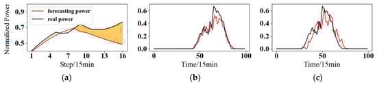
Figure 1.
Schematic diagram of PV UST results by time series forecasting: (a) Results of steps 1–16 UST forecasts compared with real power. (b) Results of 1st step UST forecasts compared with real power. (c) Results of 16th step UST forecasts compared with real power.
In recent years, advances in Numerical Weather Prediction (NWP) technology have made high-frequency intra-day forecasting feasible, with updates available as frequently as every 6 h. This development enables the integration of NWP data into USTPF models. Theoretically, incorporating intra-day NWP forecasts can help alleviate the “delay” phenomenon. Accordingly, this paper proposes a novel USTPF method for multiple PV stations, which jointly considers the temporal characteristics of historical power data and the trend features of future NWP. The main contributions of this work are as follows:
(1) Building upon the concepts of the “Fine-grained modeling”, this work proposes a unified network architecture that dynamically integrates historical power time series features with future NWP trend characteristics, which we called the Temporal Attention-Variable Parallel Encoding Fusion Network, resolving the issue of performance degradation over longer horizons for traditional time series models. The model comprises two core modules:
- Parallel encoding module for historical power and NWP data. Given the varying influence of historical power and future NWP data on power forecasting, independent encoding modules are constructed for each sequence to extract deep temporal features.
- Two-stage coupled decoding module. Considering the differential impact of historical temporal features and NWP trend features across forecasting horizons, a two-stage decoding strategy is adopted. For near-term steps, the model relies solely on temporal features, while for longer-term steps, it dynamically fuses encoded historical power information with future NWP data to accurately capture future trend dynamics.
(2) The proposed method is validated using data from six PV stations in China. Comparative experiments with state-of-the-art (SOTA) models under various weather conditions and across different stations demonstrate the effectiveness of the method for 1–16 step forecasting. Ablation studies further confirm that while maintaining high accuracy for near-term predictions, the proposed model significantly improves performance for steps 8–16.
The remainder of this paper is organized as follows: Section 2 presents the materials and methods, including the theoretical foundation and complete modeling process. Section 3 reports the results and verifies the effectiveness of the proposed method through case studies. Section 4 discusses the limitations and outlines future research directions. Section 5 provides the conclusions.
2. Materials and Methods
2.1. Theoretical Basis of TA-VPF-EN
Based on the above considerations, we propose the Temporal Attention–Variable Parallel Fusion Encoder Network (TA-VPF-EN), as illustrated in Figure 2. To better capture the mapping relationship between input and output sequences, the overall model adopts a sequence-to-sequence (seq2seq) architecture. The modeling process is as follows:
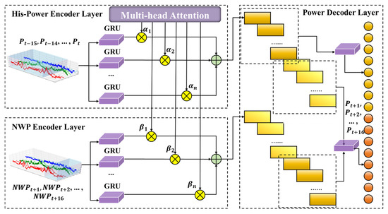
Figure 2.
Schematic diagram of TA-VPF-EN.
(1) Parallel Encoding Module for Historical Power and NWP Data. Historical power and future NWP data exert different levels of influence on forecasting results. Although both are essentially temporal sequences, their representations differ. Specifically, historical power and forecasting power exhibit an extrapolation relationship, whereas NWP data correspond to a synchronous mapping. Moreover, due to inherent errors in NWP forecasts, the mapping relationship requires certain corrections.
Therefore, independent encoding modules are constructed for the two types of sequences. Each encoding module consists of a Gated Recurrent Unit (GRU) layer and an attention mechanism. The GRU layer [17] extracts temporal features; its structure is similar to that of the LSTM [30], but with key differences. As shown in Figure 3a, the GRU merges the forget gate and input gate into a single update gate while combining the cell state and hidden state. This design simplifies the architecture, improves computational efficiency, and is well-suited for capturing temporal dependencies. The data processing procedure of this module is formulated in Equations (1)–(4), where and are input weight matrices, is current memory content, is the Hadamard operations, and is the sigmoid activation function.
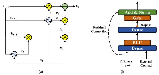
Figure 3.
Schematic diagram of GRU and GRN: (a) GRU; (b) GRN.
It is worth noting that, in order to enhance the model’s ability to recognize temporal characteristics, positional encoding is applied to both types of input sequences. The encoding method is defined in Equations (5) and (6), where PE denotes the encoded value, pos represents the index of the power point in the temporal sequence, indicates the dimension of the mapped power value, and i denotes the index within the mapping dimension. The input sequences are first processed through a fully connected layer and then combined with positional encoding to obtain the final input vectors .
Subsequently, an attention module is employed to dynamically weight the spatiotemporal features extracted by the GRU layers, thereby achieving the fusion of temporal matrices and further enhancing feature representation. The self-attention mechanism was introduced by Google in 2017 [31] and assumes that after linear mapping and positional encoding, the representation dimension of power values at each time step is d. When entering the multi-head self-attention computation layer, a fully connected network expands the representation dimension of each time step to , which is then evenly distributed across M self-attention heads. Through computation, groups of power representation vectors with dimension d are obtained. These vectors are subsequently concatenated and passed through a fully connected network to yield the final power representation vectors with dimension d, completing the Multi-Head Self-Attention process. The specific computation is defined in Equations (7)–(9), where denotes the attention-weighted result of the ith subspace group, represents the parameter matrix used during concatenation, and MH corresponds to the final weighted output.
(2) Forecast Power Decoding Layer. This module employs a two-stage coupled forecasting strategy to establish the mapping between historical power sequences, future NWP sequences, and future power outputs. Specifically, at time step t, the sequence length is set to 16, with the historical power sequence, future NWP sequence, and future power sequence denoted as , , and , respectively.
For the first 8 forecasting steps, the model relies solely on historical power data to fully exploit its strong temporal auto correlation. Two GRU modules are used to encode , and to address the dimensionality issue arising from the fusion of self-attention features, a RepeatVector is applied to expand the dimensions. The resulting representation is then mapped through a fully connected layer into an 8-step feature sequence. The overall process is formulated in Equations (10)–(12), where denotes the high-level contextual vector extracted from N input sequences, represents the decoded feature vector for the next 8 steps, and is the final forecasting power sequence for these 8 steps.
For the latter 8 forecasting steps, considering the limitations of time series forecasting and the reliability of NWP data, relying solely on either source may lead to varying degrees of performance degradation. Therefore, it is necessary to dynamically account for the influence of both on the final results. To this end, a Gated Residual Network (GRN) mechanism is introduced, as illustrated in Figure 3b. The GRN [32] combines the concepts of gating and residual connections, enabling adaptive regulation of information flow, suppression of irrelevant or noisy features, and enhancement of critical information.
The core components of the GRN consist of two dense layers and two types of activation functions: Exponential Linear Unit (ELU) and Gated Linear Unit (GLU). The ELU activation function primarily serves to suppress negative values, mitigate the vanishing gradient problem, and improve the stability of network training. The GLU, on the other hand, is mainly used to select and weight the most important features for subsequent estimation, thereby capturing relevant correlations. The detailed computational process is defined in Equations (13) and (14), where a and c denotes the main input and contextual vector, represents the corresponding weight matrix, and is the associated bias vector. , are intermediate layers.
Letting be the input, the GLU then takes the form
where represents the corresponding weight matrix, is the associated bias vector, and is the sigmoid activation function.
(3) Loss Function. After processing by the above modules, the results are concatenated, and finally a sequence matching the output data is generated through a dense layer to obtain the predicted power for the next 4 h (16 steps). To train the model, it is necessary to optimize two training objectives. This process is highly dependent on the weighting scheme between the loss functions of the two objectives. Therefore, the loss function is set by dynamic weights, as shown in Equation (16), where and are the measured value, , , and are the historical power and the predicted power obtained by NWP decoding, and , , and are the weight. The final result is determined by continuous optimization during the training process.
2.2. Modeling Process of TA-VPF-EN
To summarize, the overall modeling process is illustrated in Figure 4, with specific steps as follows:
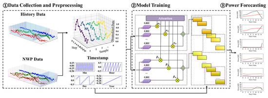
Figure 4.
Schematic diagram of modeling process.
(1) Data Collection and Preprocessing. Historical power data, meteorological data, and corresponding NWP data are collected. The data are cleaned to remove obvious anomalies records, each type of data is then normalized separately. After normalization, the dataset is split into training and testing sets.
(2) Data Reconstruction. The training and testing data are reconstructed to match the model’s input–output format. Taking a power sequence of length n as an example, the reconstruction method is shown in Equation (17), where L is the input sequence length. Through experimentation, L = 16 yields the best results, meaning the model uses the past 4 h data, next 4 h NWP irradiance, and timestamp information as input to predict the next 4 h power. Historical power, irradiance, NWP irradiance, and timestamp data [33] from each station are reconstructed according to Equation (17), denoted as , , and , where includes year, month, day, hour, and minute labels. These are then combined into as the model input, while the output only consists of power data, denoted as .
(3) TA-VPF-EN Model Training. The model parameters are initialized with as input and as output. During training, the hidden dimensions of both modules are set within the range [16–64], batch size between [256–512], and learning rate between [0.001–0.01]. Optimal parameters are determined via grid search. The number of epochs is set to 500, and the base loss function for each task is the Mean Squared Error (MSE). The Adam optimizer is used. To prevent overfitting and reduce training time, dropout and early stopping mechanisms are introduced to further enhance model performance. Training continues until the model converges.
(4) Ultra-Short-Term Power Forecasting. Every 15 min, the model takes data from time steps (t − 16) to (t − 1) as input and predicts power for time steps (t + 1) to (t + 16) using the TA-VPF-EN model. The output is then denormalized to produce the ultra-short-term forecast for the next 4 h.
3. Results
3.1. Data Set
We used data from six PV stations in northern China to validate the proposed method. The installed capacities are 100 MW, 45 MW, 30 MW, 20 MW, 20 MW, and 80 MW, respectively, and the stations are denoted PV1–PV6. Both the measured power data and the NWP data span 1 January 2024 to 31 May 2025. The power data have a 15 min resolution, while the NWP data have a 1 h resolution and are interpolated to 15 min intervals for use (by linear interpolation). The 2024 data are used as the training set, and the 2025 data are used as the test set.
3.2. Baseline Algorithms
To intuitively evaluate the forecasting performance of the proposed method, we compare it against three SOTA models widely used in USTPF: BiLSTM [34], Transformer [31], and Dlinear [35]. The input/output data types and hyperparameter selection follow the same approach described in Section 2.2; the details are shown in Table 1. All experiments were implemented in Python 3.10, running on a Windows 64-bit system with an Intel(R) Core(TM) i7-9750H CPU and 16.0 GB RAM. For simplicity, the proposed method and the four comparison models are denoted as TA-VPF-EN, case1, case2, and case3, respectively.

Table 1.
Details of model parameters.
The evaluation metrics for power prediction results include accuracy and the coefficient of determination, as defined in Equations (18) and (19), donated as A and . Here, i represents the average metric at step i, and denote the actual and predicted power at time j, is the average actual value at step i, and is the installed capacity of the corresponding station.
3.3. Forecasting Task
Following the above description, forecasting is carried out for the next 4h with a time resolution of 15 min. The 1–16 steps performance metrics are illustrated in Figure 5, while the average results across all stations are summarized in Table 2. To highlight key insights, only the results for steps 1, 4, 8, 12, and 16 are presented in the table.
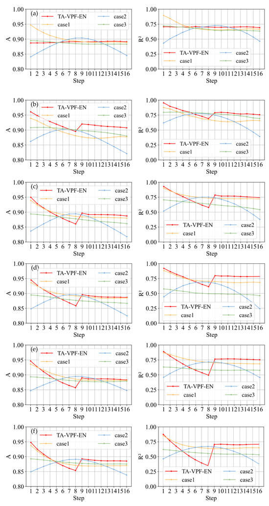
Figure 5.
A & for different cases in every PV station: (a) PV1; (b) PV2; (c) PV3; (d) PV4; (e) PV5; (f) PV6.
Table 2.
Average A & for every forecasting step in every case.
From Table 2, it is clear that TA-VPF-EN significantly outperforms the comparison models at steps 1, 12, and 16. Specifically, the A improves by 0.1 to 9.2 percentage points over case1, case2, and case3, while the shows an even more pronounced improvement of 0.4 to 41.7 percentage points, especially at steps 12 and 16. From Figure 5, we can observe the overall performance trends. Except for case2 (the blue curve, representing the Transformer model), all other models show a decline in performance as the prediction horizon increases. However, caused by the integration of NWP data, this decline is more gradual, and stable forecasting performance is maintained from steps 9 to 16. This effect is most evident in TA-VPF-EN (the red curve), which shows a noticeable rebound at step 9 and maintains stability thereafter. In contrast, case1 (yellow curve, representing the BiLSTM model) and case3 (green curve, representing the DLinear model) do not exhibit this behavior. This suggests that directly incorporating NWP data can help correct predictions, but the effect is inconsistent. In fact, case1, case2, and case3 show that unprocessed NWP inputs may disrupt temporal forecasting, especially in early steps, where accuracy drops sharply. This likely stems from the model overemphasizing NWP features and losing the advantage of extrapolating from historical power trends. Case2 is particularly affected, resulting in a convex-shaped performance curve due to imbalanced handling of historical and future data.
In contrast, TA-VPF-EN uses a tailored approach that maintains strong performance in steps 1–8 and leverages NWP data to refine predictions in the latter eight steps, validating the effectiveness of the design.
From the station perspective, TA-VPF-EN also demonstrates excellent stability. In terms of the A, the left column of subplots shows that TA-VPF-EN consistently ranks highest across all 1–16 steps, especially in the latter half, where it remains between 0.873 and 0.920, outperforming all other models. This is most evident in PV2 (subplot (b)), where TA-VPF-EN maintains accuracy above 0.9 after step 8, exceeding other models by 2.1 to 8.6 percentage points. The improvement is significant, proving that the prediction results obtained by the proposed method have smaller deviations from the actual values and are closer to the actual values. For the , TA-VPF-EN again performs strongly. The right column of subplots shows that it stays high across all steps, especially in the last eight steps, where it ranges from 0.620 to 0.820. In contrast, the comparison models peak at just 0.749, with some dropping as low as 0.144. This indicates that as the prediction horizon grows, other models struggle to follow the actual trend, while TA-VPF-EN maintains reliable trend tracking even at step 16. This highlights the value of dynamically balancing historical sequences and future NWP inputs, further confirming the method’s effectiveness.
To visually illustrate the forecasting performance, Figure 6 presents a comparison of predicted and actual power curves across stations. Since nearby steps yield similar metrics, step 16 is selected for clearer contrast. As shown in the gray dashed boxes, TA-VPF-EN successfully tracks sharp fluctuations in actual power, aligning well with earlier analysis.
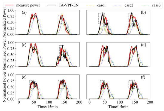
Figure 6.
WPF curves for different cases in every PV station: (a) PV1; (b) PV2; (c) PV3; (d) PV4; (e) PV5; (f) PV6.
To provide a more comprehensive evaluation of forecasting performance, violin plots of the prediction metrics for each model across all stations were generated. To emphasize key insights, only the step 16 results were included, as shown in Figure 7. The plots clearly demonstrate that TA-VPF-EN delivers more stable predictions. Specifically, for each station, the minimum, mean, and maximum lines of the violin plots for both metrics are consistently higher than those of the comparison models. For instance, in Figure 7a, PV3 and PV6 show minimum values that exceed those of other models by 1.9 to 11.9 percentage points, and mean values that are higher by 1.2 to 7.4 percentage points. From a distribution perspective, A for TA-VPF-EN is mostly concentrated above 0.85, with fewer outliers and a tighter spread, indicating strong and consistent accuracy. This conclusion is further supported by Figure 7b, where the for TA-VPF-EN is generally above 0.7, also showing a concentrated distribution. This reflects good curve fitting and stable trend tracking, confirming the robustness of the proposed method.
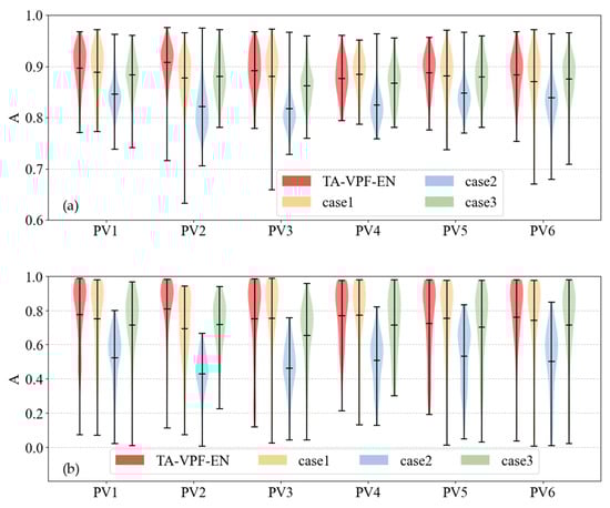
Figure 7.
Violin diagram of A & for different cases in every PV station: (a) A; (b) .
Considering that PV power is highly sensitive to weather conditions, forecasting difficulty varies significantly across different weather types, the samples are classified by day into sunny, cloudy, and rainy categories. The prediction performance of each model under these conditions is then evaluated across all stations. To highlight key insights, the analysis focuses on step 16, with results summarized in Table 3. Additionally, to visually illustrate the forecasting behavior, Figure 8 presents the predicted power curves under the three weather scenarios.
Table 3.
Average A & for every weather in every case.
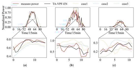
Figure 8.
WPF curves for different cases in different weather: (a) clear; (b) cloudy; (c) rainy.
Combined with the table and figure, all models exhibit a consistent error trend across weather types: sunny > rainy > cloudy, which aligns with common expectations. For more details, on sunny days, PV output curves are smooth and highly structured, making them easier to predict. All models perform well under these conditions, with both metrics reaching high levels.
On rainy days, overall PV output is lower and more volatile, increasing the forecasting difficulty. In this scenario, TA-VPF-EN shows a clear advantage, with the A improving by 1.50–7.30 percentage points and the by 0.061–0.105 compared to other models.
On cloudy days, short-term cloud movements cause frequent fluctuations in PV output, making prediction especially challenging. Even so, TA-VPF-EN maintains strong performance, with the A improving by 2.00–6.30 percentage points and the by 0.067–0.232 over the comparison models.
Together, these results demonstrate that the proposed method achieves higher accuracy and better trend tracking across diverse weather scenarios. Its ability to effectively integrate both NWP and temporal features makes it a reliable solution for UST PV power forecasting.
4. Discussion
While previous analysis confirms the effectiveness of TA-VPF-EN, the individual contributions of each module remain to be validated. To address this, ablation experiments are conducted to test the theoretical soundness of each component. These experiments are denoted as case4–case6, with their configurations detailed in Table 4, the details are as flowing:
Table 4.
Setting up method of ablation cases.
Case4 uses only historical power and irradiance data as input, reverting to a conventional time series forecasting approach. Since NWP data are excluded, parallel encoding and coupled decoding are no longer applicable and are removed accordingly.
Case5 eliminates separate encoding for NWP and power data, feeding them into the model as a combined input. Originally, the input , consisted of , and along with timestamps , while in case5, the input is simply and .
Case6 modifies the decoding process by removing the weighting mechanism. Instead of assigning explicit weights to different input types, it allows the model to handle all inputs equally during decoding.
Based on the results in Figure 9, the prediction performance across stations and models reveals distinct error patterns:
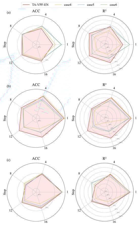
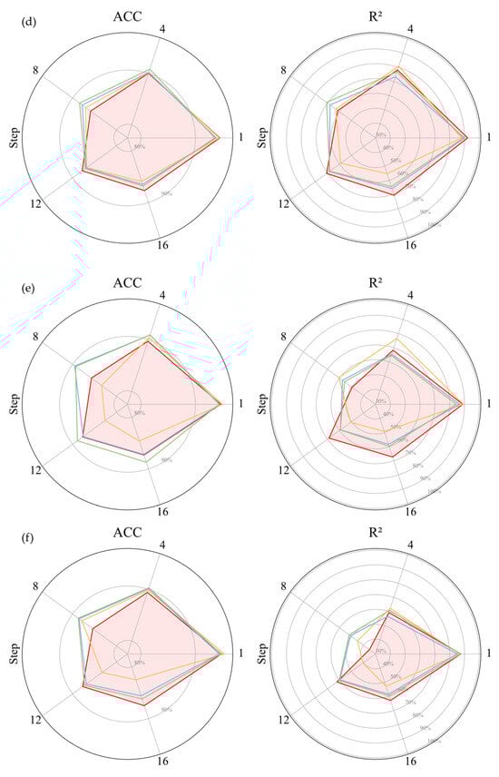
Figure 9.
Radar diagram of A & for different cases in every PV station: (a) PV1; (b) PV2; (c) PV3; (d) PV4; (e) PV5; (f) PV6.
(1) Case4 shows strong performance at step 1, especially for PV2-PV6, where the A surpasses other models by 0.20–2.50 percentage points. However, as the prediction horizon extends, its accuracy drops sharply. By step 16, case4 lags behind all other models, with the A declining by up to 5.20 percentage points and the falling by as much as 0.397. This confirms the earlier analysis: while time series models perform well in the short term, they struggle with long-term trend tracking, highlighting the importance of incorporating NWP data.
(2) Case6 exhibits the opposite trend compare to case4. Its early-step performance is relatively weak, but it stabilizes as the horizon increases. From steps 8 to 16, case6 consistently outperforms case4 and case5. Notably, in PV6, the A improves by up to 6.3 percentage points, and the improves by 0.199 compared to case4 and case5. Case5 delivers moderate performance overall. It performs better than case6 in early steps but worse than case4. In later steps, it surpasses than case4 but trails than case6.
(3) However, both case5 and case6 fall short of TA-VPF-EN in steps 12–16, indicating that without dedicated handling of NWP data, the model struggles to balance temporal and meteorological inputs. Although their transition around steps 8–9 is smoother, they fail to achieve consistent accuracy across both near and distant horizons.
These findings reinforce the effectiveness of TA-VPF-EN, which dynamically integrates NWP and historical power data to maintain balanced and reliable forecasting across all time steps.
TA-VPF-EN achieves strong forecasting performance overall, but the results reveal a notable dip between steps 8 and 9, likely due to the simplistic breakpoint design between temporal and NWP feature extraction. This causes a sharp shift in prediction behavior, making the error metrics less stable compared to models that treat all inputs uniformly.
Regarding the issue of timeliness, due to incorporating parallel encoding and two-stage decoding, the TA-VPF-EN model’s training time is indeed significantly longer than the comparison models, requiring approximately 1.5 h. In contrast, the BiLSTM, Transformer, and DLinear models require only about 0.5 h, 0.75 h, and 0.1 h, respectively. However, that training is an offline process with no impact on online prediction latency. During actual forecasting, all models exhibit comparable sub-second inference times, substantially shorter than the scheduling cycle for ultra-short-term forecasting (15 min). Consequently, despite the model’s relatively complex architecture, its inference efficiency fully satisfies real-time requirements in practical engineering applications.
For future work, it would be valuable to explore adaptive breakpoint strategies, potentially treating the breakpoint as a learnable parameter within the model. This would allow dynamic optimization during training, helping the model maintain consistent performance across all 1–16 steps.
Additionally, since PV forecasting tends to be relatively straightforward, and even direct use of NWP yields decent results, it is worth considering an extension of the method to more stochastic scenarios, which includes incorporating datasets that exhibit greater spatial heterogeneity, such as southern or northern regions, coastal or inland areas, or using for wind power forecasting. This would provide a more rigorous test of the model’s robustness and further validate its design under complex, high-variability conditions.
5. Conclusions
This study addresses the challenge of rapid accuracy decay in traditional UST PV power forecasting methods, which rely solely on historical data. By innovatively incorporating near-term NWP forecast data to dynamically correct time series predictions, the proposed approach effectively mitigates the accuracy drop in 3–4 h forecasts. The main contributions are as follows:
(1) The TA-VPF-EN model is proposed: The model features a parallel encoding module that extracts deep temporal features from both historical power data and future NWP inputs. A two-stage coupled decoding mechanism is employed, relying on pure time series features for near-term predictions and dynamically integrating historical power encoding with future NWP trends for longer horizons. This design accurately captures power variation patterns across different time scales.
(2) Using empirical validation across six PV stations in China, compared to SOTA models, the proposed method reduces the average NRMSE by 0.50–5.20% and improves the by 0.047–0.362 in 4 h UST forecasts. It significantly enhances prediction accuracy for steps 8–16 while maintaining strong performance in earlier steps.
Overall, the proposed method offers an effective solution for multi-station PV power forecasting and holds practical significance for ensuring the safe and stable operation of power systems under high renewable energy penetration, it also possesses significant economic value.
Economic value for grid dispatch and stable operation: More accurate UST forecasts, particularly corrections for power fluctuations over the next 3–4 h (such as peak delays) enable grid dispatchers to allocate reserve capacity (rotating reserve, fast frequency regulation resources) with greater precision. This reduces excess or insufficient reserves caused by forecasting errors, thereby lowering system balancing costs and enhancing grid operational security and economic efficiency under high renewable energy penetration.
Potential value for electricity markets and arbitrage: In regions implementing time-of-use pricing or spot markets, precise power forecasting forms the foundation for market participation and revenue optimization. The model’s significant improvement in forecasting performance for the next 2–4 h enables PV site operators to more accurately predict their generation capacity during critical market periods. This facilitates the development of superior bidding strategies, increasing opportunities and returns from price arbitrage.
Contribution to PV Site Operational Efficiency: Accurate power forecasting aids in optimizing site maintenance schedules and provides more reliable inputs for coordinated control of inverters and energy storage systems. This enhances the overall energy utilization efficiency of the entire generation system.
Author Contributions
Conceptualization, J.Z. and C.G.; methodology, Z.Z.; software, R.G., X.H. and C.G.; validation, X.H., C.G. and T.Q.; formal analysis, C.G.; investigation, J.Z.; resources, J.Z.; data curation, J.Z., Z.Z., R.G. and X.H.; writing—original draft preparation, J.Z. and Z.Z.; writing—review and editing, C.G. and J.Y.; visualization, J.Z. and T.Q.; supervision, J.Z. and C.G.; project administration, J.Z. and J.Y.; funding acquisition, J.Z. All authors have read and agreed to the published version of the manuscript.
Funding
This research was funded by China Meteorological Administration Special Innovation and Development Program, grant number CXFZ2024J038.
Data Availability Statement
We regret that due to privacy, we are unable to provide the data used in the paper.
Conflicts of Interest
Author Tonghui Qu was employed by the company Powerchina Jilin Electric Power Survey and Design Institute Corporation Limited. The remaining authors declare that the research was conducted in the absence of any commercial or financial relationships that could be construed as a potential conflict of interest.
Abbreviations
The following abbreviations are used in this manuscript:
| ELU | Exponential Linear Unit |
| GLU | Gated Linear Unit |
| GRN | Gated Residual Network |
| GRU | Gated Recurrent Unit |
| LSTM | Long Short-Term Memory |
| NRMSE | Normalized Root Mean Square Error |
| NWP | Numerical Weather Prediction |
| PV | Photovoltaic |
| seq2seq | Sequence to sequence |
| SOTA | State of the art |
| TA-VPF-EN | Temporal Attention Variable Parallel Fusion Encoder Network |
| UST | Ultra Short Term |
| USTPF | Ultra-Short-Term Power Forecasting |
References
- Jia, R.; He, M.; Zhang, X.; Zhao, Z.; Han, S.; Jurasz, J.; Chen, D.; Xu, B. Optimal Operation of Cascade Hydro-Wind-Photovoltaic Complementary Generation System with Vibration Avoidance Strategy. Appl. Energy 2022, 324, 119735. [Google Scholar] [CrossRef]
- Yan, J.; Zhang, H.; Liu, Y.; Han, S.; Li, L.; Lu, Z. Forecasting the High Penetration of Wind Power on Multiple Scales Using Multi-to-Multi Mapping. IEEE Trans. Power Syst. 2017, 33, 3276–3284. [Google Scholar] [CrossRef]
- Yang, Y.; Fan, S.; Liu, Z.; Yu, Z. WD-SGformer: High-Precision Wind Power Forecasting via Dual-Attention Dynamic Spatio-Temporal Learning. Energy 2025, 337, 138538. [Google Scholar] [CrossRef]
- Lu, P.; Ye, L.; Zhao, Y.; Dai, B.; Pei, M.; Tang, Y. Review of Meta-Heuristic Algorithms for Wind Power Prediction: Methodologies, Applications and Challenges. Appl. Energy 2021, 301, 117446. [Google Scholar] [CrossRef]
- Peng, X.; Xiong, L.; Wen, J.Y.; Cheng, S.J.; Deng, D.Y.; Feng, S.L.; Wang, B. A Summary of the State of the Art for Short-Term and Ultra-Short-Term Wind Power Prediction of Regions. Proc. CSEE 2016, 36, 6315–6326. [Google Scholar]
- Kong, W.; Jia, Y.; Dong, Z.Y.; Meng, K.; Chai, S. Hybrid Approaches Based on Deep Whole-Sky-Image Learning to Photovoltaic Generation Forecasting. Appl. Energy 2020, 280, 115875. [Google Scholar] [CrossRef]
- Qu, B.; Xing, Z.; Liu, Y.; Chen, L. Research on Short-term Output Power Forecast Model of Wind Farm Based on Neural Network Combination Algorithm. Wind Energy 2022, 25, 1710–1734. [Google Scholar] [CrossRef]
- Wang, C.-H.; Zhao, Q.; Tian, R. Short-Term Wind Power Prediction Based on a Hybrid Markov-Based PSO-BP Neural Network. Energies 2023, 16, 4282. [Google Scholar] [CrossRef]
- Mercier, T.M.; Sabet, A.; Rahman, T. Vision Transformer Models to Measure Solar Irradiance Using Sky Images in Temperate Climates. Appl. Energy 2024, 362, 122967. [Google Scholar] [CrossRef]
- Shi, J.; Lee, W.-J.; Liu, Y.; Yang, Y.; Wang, P. Forecasting Power Output of Photovoltaic Systems Based on Weather Classification and Support Vector Machines. IEEE Trans. Ind. Appl. 2012, 48, 1064–1069. [Google Scholar] [CrossRef]
- Emamian, M.; Eskandari, A.; Aghaei, M.; Nedaei, A.; Sizkouhi, A.M.; Milimonfared, J. Cloud Computing and IoT Based Intelligent Monitoring System for Photovoltaic Plants Using Machine Learning Techniques. Energies 2022, 15, 3014. [Google Scholar] [CrossRef]
- Gutiérrez, L.; Patiño, J.; Duque-Grisales, E. A Comparison of the Performance of Supervised Learning Algorithms for Solar Power Prediction. Energies 2021, 14, 4424. [Google Scholar] [CrossRef]
- Zeng, J.; Qiao, W. Short-Term Wind Power Prediction Using a Wavelet Support Vector Machine. IEEE Trans. Sustain. Energy 2012, 3, 255–264. [Google Scholar] [CrossRef]
- Li, K.; Wang, F.; Mi, Z.; Fotuhi-Firuzabad, M.; Duić, N.; Wang, T. Capacity and Output Power Estimation Approach of Individual Behind-the-Meter Distributed Photovoltaic System for Demand Response Baseline Estimation. Appl. Energy 2019, 253, 113595. [Google Scholar] [CrossRef]
- Chen, S.; Li, C.; Xie, Y.; Li, M. Global and Direct Solar Irradiance Estimation Using Deep Learning and Selected Spectral Satellite Images. Appl. Energy 2023, 352, 121979. [Google Scholar] [CrossRef]
- Yu, J.; Li, X.; Yang, L.; Li, L.; Huang, Z.; Shen, K.; Yang, X.; Yang, X.; Xu, Z.; Zhang, D. Deep Learning Models for PV Power Forecasting. Energies 2024, 17, 3973. [Google Scholar] [CrossRef]
- Huang, H.-H.; Huang, Y.-H. Applying Green Learning to Regional Wind Power Prediction and Fluctuation Risk Assessment. Energy 2024, 295, 131057. [Google Scholar] [CrossRef]
- Browell, J.; Drew, D.R.; Philippopoulos, K. Improved Very Short-term Spatio-temporal Wind Forecasting Using Atmospheric Regimes. Wind Energy 2018, 21, 968–979. [Google Scholar] [CrossRef]
- Brown, B.G.; Katz, R.W.; Murphy, A.H. Time Series Models to Simulate and Forecast Wind Speed and Wind Power. J. Appl. Meteorol. Climatol. 1984, 23, 1184–1195. [Google Scholar] [CrossRef]
- Reikard, G.; Robertson, B.; Bidlot, J.-R. Combining Wave Energy with Wind and Solar: Short-Term Forecasting. Renew. Energy 2015, 81, 442–456. [Google Scholar] [CrossRef]
- Kang, Z.; Xue, J.; Lai, C.S.; Wang, Y.; Yuan, H.; Xu, F. Vision Transformer-Based Photovoltaic Prediction Model. Energies 2023, 16, 4737. [Google Scholar] [CrossRef]
- Liu, X.; Yang, L.; Zhang, Z. Short-Term Multi-Step Ahead Wind Power Predictions Based on a Novel Deep Convolutional Recurrent Network Method. IEEE Trans. Sustain. Energy 2021, 12, 1820–1833. [Google Scholar] [CrossRef]
- Bandara, K.; Bergmeir, C.; Smyl, S. Forecasting across Time Series Databases Using Recurrent Neural Networks on Groups of Similar Series: A Clustering Approach. Expert Syst. Appl. 2020, 140, 112896. [Google Scholar] [CrossRef]
- Zhang, J.; Liu, D.; Li, Z.; Han, X.; Liu, H.; Dong, C.; Wang, J.; Liu, C.; Xia, Y. Power Prediction of a Wind Farm Cluster Based on Spatiotemporal Correlations. Appl. Energy 2021, 302, 117568. [Google Scholar] [CrossRef]
- Trull, O.; García-Díaz, J.C.; Peiró-Signes, A. A Comparative Study of Statistical and Machine Learning Methods for Solar Irradiance Forecasting Using the Folsom PLC Dataset. Energies 2025, 18, 4122. [Google Scholar] [CrossRef]
- Choi, S.; Hur, J. An Ensemble Learner-Based Bagging Model Using Past Output Data for Photovoltaic Forecasting. Energies 2020, 13, 1438. [Google Scholar] [CrossRef]
- Severiano, C.A.; de Lima e Silva, P.C.; Cohen, M.W.; Guimarães, F.G. Evolving Fuzzy Time Series for Spatio-Temporal Forecasting in Renewable Energy Systems. Renew. Energy 2021, 171, 764–783. [Google Scholar] [CrossRef]
- Zhang, Y.; Yan, J.; Han, S.; Liu, Y.; Song, Z. Joint Forecasting of Regional Wind and Solar Power Based on Attention Neural Network. In Proceedings of the 2022 IEEE 5th International Electrical and Energy Conference (CIEEC), Nanjing, China, 27–29 May 2022; pp. 4165–4169. [Google Scholar]
- Chen, Y.; Xiao, J.-W.; Wang, Y.-W.; Li, Y. Regional Wind-Photovoltaic Combined Power Generation Forecasting Based on a Novel Multi-Task Learning Framework and TPA-LSTM. Energy Convers. Manag. 2023, 297, 117715. [Google Scholar] [CrossRef]
- Ge, C.; Yan, J.; Zhang, H.; Li, Y.; Wang, H.; Liu, Y. Joint Short-Term Power Forecasting of Hydro-Wind-Photovoltaic Considering Spatiotemporal Delay of Weather Processes. Renew. Energy 2024, 237, 121679. [Google Scholar] [CrossRef]
- Vaswani, A.; Shazeer, N.; Parmar, N.; Uszkoreit, J.; Jones, L.; Gomez, A.N.; Kaiser, Ł.; Polosukhin, I. Attention Is All You Need. Adv. Neural Inf. Process. Syst. 2017, 30. [Google Scholar] [CrossRef]
- Li, Y.; Wang, H.; Yan, J.; Ge, C.; Han, S.; Liu, Y. Ultra-Short-Term Wind Power Forecasting Based on the Strategy of “Dynamic Matching and Online Modeling”. IEEE Trans. Sustain. Energy 2024, 16, 107–123. [Google Scholar] [CrossRef]
- Zhou, H.; Zhang, S.; Peng, J.; Zhang, S.; Li, J.; Xiong, H.; Zhang, W. Informer: Beyond Efficient Transformer for Long Sequence Time-Series Forecasting. In Proceedings of the AAAI Conference on Artificial Intelligence, Virtual, 2–9 February 2021; Volume 35, pp. 11106–11115. [Google Scholar]
- Michael, N.E.; Bansal, R.C.; Ismail, A.A.A.; Elnady, A.; Hasan, S. A Cohesive Structure of Bi-Directional Long-Short-Term Memory (BiLSTM)-GRU for Predicting Hourly Solar Radiation. Renew. Energy 2024, 222, 119943. [Google Scholar] [CrossRef]
- Liu, J.; Gong, C.; Chen, S.; Zhou, N. Multi-Step-Ahead Wind Speed Forecast Method Based on Outlier Correction, Optimized Decomposition, and Dlinear Model. Mathematics 2023, 11, 2746. [Google Scholar] [CrossRef]
Disclaimer/Publisher’s Note: The statements, opinions and data contained in all publications are solely those of the individual author(s) and contributor(s) and not of MDPI and/or the editor(s). MDPI and/or the editor(s) disclaim responsibility for any injury to people or property resulting from any ideas, methods, instructions or products referred to in the content. |
© 2026 by the authors. Licensee MDPI, Basel, Switzerland. This article is an open access article distributed under the terms and conditions of the Creative Commons Attribution (CC BY) license.