Partial Discharge Pattern Recognition of GIS with Time–Frequency Energy Grayscale Maps and an Improved Variational Bayesian Autoencoder

Abstract

Partial discharge pattern recognition is a crucial task for assessing the insulation condition of Gas-Insulated Switchgear (GIS). However, the on-site environment presents challenges such as strong electromagnetic interference, leading to acquired signals with a low signal-to-noise ratio (SNR). Furthermore, traditional pattern recognition methods based on statistical parameters suffer from redundant and inefficient features that compromise classification accuracy, while existing artificial-intelligence-based classification methods lack the ability to quantify the uncertainty in defect classification. To address these issues, this paper proposes a novel GIS partial discharge pattern recognition method based on time–frequency energy grayscale maps and an improved variational Bayesian autoencoder. Firstly, a denoising-based approximate message passing algorithm is employed to sample and denoise the discharge signals, which enhances the SNR while simultaneously reducing the number of sampling points. Subsequently, a two-dimensional time–instantaneous frequency energy grayscale map of the discharge signal is constructed based on the Hilbert–Huang Transform and energy grayscale mapping, effectively extracting key time–frequency features. Finally, an improved variational Bayesian autoencoder is utilized for the unsupervised learning of the image features, establishing a GIS defect classification method with an associated confidence level by integrating probabilistic features. Validation based on measured data demonstrates the effectiveness of the proposed method.

1. Introduction

As a key piece of equipment in modern power systems, the insulation condition of gas-insulated substations (GIS) is directly related to the stability and safety of power supply [1,2,3,4,5]. When insulation defects occur inside GIS equipment, a local electric field concentration is induced, leading to gas ionization and the occurrence of partial discharge (PD). Partial discharge is not only a major cause of insulation breakdown in high-voltage electrical equipment but also a critical indicator of insulation degradation. Owing to its anti-interference advantages in the frequency band of 300 MHz–3 GHz, the ultra-high-frequency (UHF) detection technology has become the preferred solution for high-voltage scenarios such as GIS equipment and transformers.

Numerous studies have shown that UHF signals of GIS partial discharge inevitably contain various types of noise, including periodic narrowband interference, white noise, and colored noise [6,7]. Existing studies have adopted various signal processing methods for noise reduction, such as wavelet transform [8,9], empirical mode decomposition (EMD) [10,11], singular value decomposition (SVD) [12,13], and multi-channel joint technology [14]. Wavelet transform and SVD show significant effects only on Gaussian noise and narrowband interference, respectively. EMD involves excessive iterations, and easily produces unexplainable decomposed modes. Multi-channel joint technology has high equipment costs and is not suitable for old GIS. And the adaptability of existing denoising methods to complex multi-noise scenarios is insufficient.

In the field of feature extraction from partial discharge data, researchers both in China and abroad have investigated the use of various PD feature values and combinations of features for PD pattern recognition. Among these, the most traditional and widely used approach is the mathematical statistics of the phase characteristics of discharge pulses [15,16,17,18]. Reference [15] realized the pattern classification and recognition of partial discharge by counting features such as the number and amplitude of pulses in each phase, and then using K-means clustering. With the development of image feature extraction and deep learning classification algorithms, the research focus of GIS PD pattern recognition has gradually shifted to intelligent image classification algorithms based on deep learning. For phase-resolved partial discharge (PRPD) spectra and phase-resolved pulse sequence (PRPS) spectra, the existing studies have employed deep learning algorithms such as convolutional neural networks (CNNs) [19,20], long short-term memory (LSTM) [21,22], traditional VAE [23], and deep belief networks (DBNs) [24] for PD pattern classification and recognition. However, phase-based spectra depend on long-term manual interpretation experience, resulting in the poor reproducibility of recognition results [25,26], and existing AI-based methods lack the ability to quantify classification uncertainty.

In conclusion, the existing methods still have the drawback of the poor adaptability of denoising techniques, over-reliance on expert experience and phase information for feature extraction, and lack of classification uncertainty quantification. To address these issues, this study proposes a deep learning method for PD pattern recognition based on approximate message passing and time–frequency energy grayscale images. First, denoiser-based approximate message passing (D-AMP) is used to perform the efficient sampling and denoising of PD UHF signals. Under the dual conditions of a suitable measurement matrix and stable iterative convergence, the Onsager correction term in D-AMP permits the effective noise to be approximated as Gaussian. This enables the method to maintain a robust denoising performance across multiple noise types. Subsequently, the Hilbert–Huang transform (HHT) is applied to extract the time–instantaneous frequency energy map of the reconstructed PD signals, which is then converted into a two-dimensional time–frequency energy grayscale image through normalization and mapping. Finally, the time–frequency energy grayscale image is used as the input to train the improved variational Bayesian autoencoder (IVBAE), and the trained model is employed to recognize PD patterns and output classification results along with confidence probabilities.

The remainder of the paper is organized as follows: Section 2 introduces the detailed procedures of the PD-UHF signal sampling and denoising method based on D-AMP. Section 3 illustrates the proposed PD pattern recognition model based on the time–frequency energy grayscale images and improved variational Bayesian autoencoder. In Section 4, case studies are performed, and Section 5 summarizes the paper.

2. The Design of PD-UHF Signal Sampling and Denoising Method Based on D-AMP

2.1. The Framework of D-AMP

Essentially, D-AMP combines the noise suppression capability of a denoiser with the efficient iterative reconstruction performance of approximate message passing (AMP). Its core innovation lies in the Onsager correction term: by compensating for the noise deviation introduced by the correlation of the measurement matrix, the effective noise during the iterative process always follows a Gaussian distribution, thereby adapting to the design assumption of the denoiser (denoisers are usually optimized for additive white Gaussian noise (AWGN)) [27].

For high-dimensional signals (discretized vectors of PD-UHF signals), the iterative process of D-AMP consists of three parts: the signal estimation update, residual update, and noise standard deviation estimation. The core formulae are as follows:

$$\left\{\begin{array}{l}{x}^{t+1}=D_{{\widehat{\sigma }}^t}\left(x^t+A^{*}{z}^t\right)\hfill \\ z^t=y-A{x}^t+z^{t-1}\cdot {\displaystyle \frac{\mathit{div}{D}_{{\widehat{\sigma }}^{t-1}}\left(x^{t-1}+A^{*}{z}^{t-1}\right)}{m}}\hfill \\ {\left({\widehat{\sigma }}^t\right)}^2={\displaystyle \frac{{‖z^t‖}_2^2}{m}}\hfill \end{array}\right.$$

(1)

where $x^t$ is the PD-UHF signal estimation vector at the t-th iteration step, and $x_0$ is the real noise-free signal; $y\in {\mathrm{R}}^m$ is the compressed measurement vector, and $A\in {\mathrm{R}}^{m\times n}$ is the measurement matrix; $z^t$ is the residual vector, which reflects the deviation between the current estimation and the measured value; $\mathit{div}D$ is the divergence of the denoiser $D$; and $D_{{\widehat{\sigma }}^t}$ is the denoiser adapted to the noise standard deviation, which is estimated from the energy of the residual vector ${\widehat{\sigma }}^t$.

It should be noted that the Gaussian approximation of the effective noise via the Onsager correction term relies on two key prerequisites: (1) the measurement matrix must satisfy the restricted isometry property (RIP) to prevent signal distortion during compressive sampling; and (2) the D-AMP iteration must converge stably, which allows the Onsager term to continuously counteract the bias introduced by correlations in the measurement matrix. Only under these conditions can the effective noise during iteration be reasonably approximated as Gaussian, thereby aligning with the statistical assumption underlying the BM3D denoiser. This approximation is not universally applicable to arbitrary noise types or system configurations, but is valid within the experimental and parametric framework of the present study.

2.2. The Denoising of PD-UHF Signals

The denoiser is the core of D-AMP performance and needs to balance the non-local self-similarity of PD-UHF signals (consistent waveform structures of different PD pulses) and the sensitivity to time-domain details (pulse amplitude and rising edge contain defect information). An improved block matching 3D (BM3D) denoiser is selected, denoted as $D_{\sigma }^{\mathit{BM}3D\text{-}\mathit{PD}}$, and optimized according to the characteristics of PD-UHF signals.

2.2.1. Adaptability Analysis of BM3D

BM3D achieves the collaborative filtering of non-locally similar blocks through “block matching–3D transformation–threshold shrinking–inverse transformation”, which can effectively suppress Gaussian noise and retain signal details. However, the original BM3D is designed for images and requires the following improvements for PD-UHF time-domain signals: 1. A hybrid transformation basis of “time-domain discrete cosine transform (DCT) and pulse feature dimension wavelet transform” is adopted to compress the redundant information within the block. 2. An adaptive soft threshold is used to address the pulse amplitude differences of PD-UHF signals:

$$\tau (\sigma )=\alpha \cdot \sigma \cdot \sqrt{\log n}$$

(2)

where $\alpha$ is the threshold coefficient, determined through cross-validation.

2.2.2. The Calculation of Denoiser Divergence

The Onsager correction term requires the divergence of the denoiser, but $D_{\sigma }^{\mathit{BM}3D\text{-}\mathit{PD}}$ has no explicit expression. The Monte Carlo approximation method is used for the calculation:

Generate one independent and identically distributed Gaussian vector $b~\mathcal{N}(0,I)$. Take a small disturbance ($ϵ=\Vert u^t{\Vert }_{\infty }/1000$, $u^t=x^t+A^{*}{z}^t$) to avoid numerical overflow. The approximation formula for divergence is as follows:

$$\mathit{div}{D}_{{\widehat{\sigma }}^t}(u^t)\approx {\displaystyle \frac{1}{ϵ}}{b}^T\left[D_{{\widehat{\sigma }}^t}(u^t+ϵb)-D_{{\widehat{\sigma }}^t}(u^t)\right]$$

(3)

2.3. The Iterative Process of D-AMP

A complete iterative procedure is designed for the sampling and denoising of PD-UHF signals.

Set the initial value of the signal estimation to $x^0=0\in {\mathrm{R}}^n$, and the initial residual value to $z^0=y$—the initial residual is equal to the measurement vector, and set the number of iterations to $T=25$.

Construction of effective signal: Calculate $t=0,1,\dots ,T-1$; $A^{*}$ is the conjugate transpose of $A$;

Denoiser filtering: Input $u^t$ into $D_{{\widehat{\sigma }}^t}^{\mathit{BM}3D\text{-}\mathit{PD}}$ to obtain the updated signal estimation value $u^t=x^t+A^{*}{z}^t$;

Calculation of Onsager correction term: Calculate $\mathit{div}{D}_{{\widehat{\sigma }}^t}(u^t)$ using the Monte Carlo method;

Residual update: Substitute the Onsager correction term to update the residual $z^t$;

Estimation of noise standard deviation: Calculate ${\widehat{\sigma }}^t=\sqrt{\Vert z^t{\Vert }_2^2/m}$, which provides the noise intensity adaptation basis for the denoiser in the next iteration.

The iteration is terminated when either of the following conditions is met: the convergence of relative error $\Vert x^{t+1}-x^t{\Vert }_2/\Vert x^t{\Vert }_2<{10}^{-4}$; or the number of iterations reaches $T=25$.

2.4. Parameter Optimization of D-AMP Based on State Evolution

Using the state evolution theory of D-AMP, the mean square error (MSE) of the PD-UHF signal during the iterative process is predicted to optimize the key parameters: sampling rate $\delta$ and threshold coefficient $\alpha$. Define the state variable as follows ${\theta }^t={\displaystyle \frac{1}{n}}\Vert x^t-x_0{\Vert }_2^2$, and its evolution equation is as follows:

$${\theta }^{t+1}={\displaystyle \frac{1}{n}}\mathbb{E}{‖D_{{\sigma }^t}^{\mathit{BM}3D\text{-}\mathit{PD}}\left(x_0+{\sigma }^tϵ\right)-x_0‖}_2^2$$

(4)

where ${\sigma }^t=\sqrt{{\theta }^t/\delta +{\sigma }_w^2}$,$ϵ~\mathcal{N}(0,I)$.

Optimization of sampling rate: Fix $\alpha$ = 1.4, traverse $\delta \in [0.2,0.5]$, and select the $\delta$ that minimizes the steady-state MSE; experiments show that the optimal $\delta$ for PD-UHF signals is 0.5. Optimization of threshold coefficient: Fix $\delta =0.5$, traverse $\alpha \in [1.0,1.8]$, and select the $\alpha$ that minimizes the PD pulse amplitude error; experiments show that $\alpha =1.4$ is optimal.

3. PD Pattern Recognition Method Based on Time–Frequency Energy Grayscale Images and Improved Variational Bayesian Autoencoder

3.1. The Construction of Time–Frequency Energy Grayscale Images for PD Signals

The UHF detection signal of gas-insulated switchgear is a typical nonlinear and non-stationary signal. The HHT is used to analyze the time–frequency characteristics of the UHF signal and construct the time–frequency energy grayscale image [28]. The basic process is as follows:

Step 1: The high-frequency carrier of the UHF signal obscures the intensity variation of the PD pulse. Therefore, the envelope must be extracted to reveal the underlying discharge trend [29]. First, the Hilbert transform is performed on the denoised UHF signal to construct an analytic signal $z(t)$, as follows:

$$z(t)=s(t)+j\cdot \widehat{s}(t)=s(t)+{\displaystyle \frac{j}{\pi }}{\displaystyle {\int }_{-\infty }^{+\infty }\frac{s(\tau )}{t-\tau }}d\tau$$

(5)

where $s(t)$ is the denoised UHF signal, and $\widehat{s}(t)$ is its Hilbert transform. By calculating the modulus of the analytic signal, the envelope signal $x(t)$ is obtained to represent the periodic variation of the signal intensity:

$$x(t)=\sqrt{s{(t)}^2+\widehat{s}{(t)}^2}$$

(6)

During the compressed-sensing process of the UHF signal, the sampling rate is reduced within a controlled range (optimized via D-AMP parameter tuning). Although minor waveform distortions may occur, the dominant trend of the discharge-pulse envelope is preserved sufficiently to support reliable subsequent feature extraction.

Step 2: Perform EMD on the preprocessed $x(t)$, and retain the effective intrinsic mode function (IMF) components related to the PD signal through screening to eliminate redundant components dominated by noise.

Performing EMD on the envelope signal $x(t)$ can decompose the envelope into multiple IMFs from low frequency to high frequency, i.e.,

$$x(t)=r_n(t)+{\displaystyle \sum _{i=1}^{n-1}{c}_i}(t)$$

(7)

where $r_n(t)$ is the residual function, representing the average variation trend of the signal; and $c_i(t)$ is the IMF component, which contains the components of the envelope signal at different time characteristic scales.

Perform the Hilbert transform on each IMF component $c_i\left(t\right)$ to extract the instantaneous parameters for constructing the time–frequency characteristics. The calculation formula is as follows:

$$A_i(t)=c_i(t)+j{\widehat{c}}_i(t)=a_i(t)e^{j{\theta }_i(t)}$$

(8)

$$a_i(t)=\sqrt{c_i^2(t)+{\widehat{c}}_i^2(t)}$$

(9)

$${\theta }_i(t)=\arctan ({\widehat{c}}_i(t)/c_i(t)$$

(10)

where $j$ is the imaginary unit; $a_i(t)$ is the instantaneous amplitude, reflecting the intensity of the i-th IMF; and ${\theta }_i(t)$ is the instantaneous phase, reflecting the phase variation of the signal.

The instantaneous frequency is defined as the derivative of the phase with respect to time, reflecting the dynamic frequency characteristics of the IMF:

$$f_i(t)={\displaystyle \frac{1}{2\pi }}\cdot {\displaystyle \frac{d{\theta }_i(t)}{dt}}$$

(11)

where the unit of $f_i(t)$ is GHz, which can accurately capture the instantaneous frequency fluctuation of the PD pulse [30].

Step 3: Construction of Hilbert amplitude spectrum: Ignore the residual function $r_n\left(t\right)$, and the Hilbert amplitude spectrum $H\left(f,t\right)$ of the UHF signal is the superposition of the instantaneous amplitudes of all IMFs:

$$H(f,t)=\mathit{Re}\left[{\displaystyle \sum _{i=1}^{n-1}{a}_i}(t)e^{j2\pi {\displaystyle \int f_i}(t)dt}\right]$$

(12)

Construction of discrete Hilbert amplitude spectrum: The sampling of UHF signals is a discrete process. Let the sampling rate be $f_s$ and the time sequence be $t_q=q\Delta t$; set the frequency range to 0.3~2.5 GHz and the frequency interval to $\Delta f$. The discrete Hilbert amplitude spectrum is expressed in matrix form:

$$H_{xy}=\left[\begin{array}{cccc}{h}_{11}& h_{12}& \dots & h_{1Nt}\\ h_{21}& h_{22}& \dots & h_{2Nt}\\ ⋮& ⋮& \ddots & ⋮\\ h_{Nf1}& h_{Nf2}& \dots & h_{NfNt}\end{array}\right]$$

(13)

where $H\in {\mathrm{R}}^{Q\times F}$ is the discrete matrix of $H_{xy}$; $h_{pq} = H \left(fp, tq\right)$ represents the amplitude intensity at frequency $f$ at time $tq$; and the edge elements of the matrix are set to 0 to avoid interference from invalid frequencies.

Calculation of discrete time–frequency energy matrix: The energy of the UHF signal is proportional to the square of the instantaneous amplitude. Based on the discrete Hilbert amplitude spectrum $H_{xy}$, the discrete time–frequency energy matrix $E_{xy}$ is constructed:

$$E_{pq}=a_i^2(tq)\cdot \delta (fp-f_i(tq))$$

(14)

where $E_{pq}$ is the energy value at frequency $fp$ at time $tq$. $fp$ is the Dirac function—i.e., if $f_{i }\left(tq\right)\in \left[fp-\Delta f/2, fp+\Delta f/2\right]$, then $\delta (fp-f_i(t_q))=1$; otherwise $\delta (fp-f_i(t_q))=0$. $a_{i }\left(tq\right)$ is the instantaneous amplitude of the i-th IMF at time $tq$ (calculated by Equation (9)).

The final discrete time–frequency energy matrix is as follows:

$$E_{xy}=\left[\begin{array}{cccc}{E}_{11}& E_{12}& \dots & E_{1Nt}\\ E_{21}& E_{22}& \dots & E_{2Nt}\\ ⋮& ⋮& \ddots & ⋮\\ E_{Nf1}& E_{Nf2}& \dots & E_{NfNt}\end{array}\right]$$

(15)

where $E_{xy}$ has the same dimension as $H_{xy}$; and $E_{pq}\ge 0$—the higher the energy, the larger the value of $E_{pq}$.

Step 4: Conversion to energy grayscale image: To convert the discrete time–frequency energy matrix $E_{xy}$ into a grayscale image, normalization and grayscale mapping are required to ensure the comparability of the grayscale characteristics among different UHF signals.

Energy normalization: The UHF signal energies of different PD defects vary significantly. Normalization is used to map $E_{pq}$ to the interval [0, 1]:

$$E_{\mathit{norm}}(p,q)={\displaystyle \frac{E_{pq}-\min (E_{xy})}{\max (E_{xy})-\min (E_{xy})}}$$

(16)

where $E_{\mathit{norm}}(p,q)$ is the normalized energy value; $\max (E_{xy})$ and $\min (E_{xy})$ are the maximum and minimum values of $E_{xy}$, respectively; and normalization can eliminate the energy scale difference.

Grayscale value mapping: The pixel value range of a grayscale image is 0~255. Linearly map $E_{\mathit{norm}}(p,q)$ to the grayscale value:

$$G(p,q)=\mathit{round}(255\cdot E_{\mathit{norm}}(p,q))$$

(17)

where $round (\cdot )$ is the rounding function; and $G(p,q)$ is the grayscale value at position $(p,q)$. The higher the energy is, the closer the grayscale value is to 255 (white), which corresponds to the energy concentration area of the PD pulse; the lower the energy is, the closer the grayscale value is to 0 (black), which corresponds to the background noise area.

3.2. The Improved Variational Bayesian Autoencoder

IVBAE adopts a symmetric encoder–decoder architecture. It mainly consists of four parts: the patch feature extraction module, variational encoding module, hybrid latent space module, and decoding reconstruction module. These modules work together to realize feature dimensionality reduction and probability modeling [31,32,33].

The input layer receives the single-channel time–frequency energy grayscale image generated $X\in {\mathrm{R}}^{H\times W\times 1}$ by the Hilbert–Huang transform, where H and W are the height (time dimension) and width (frequency dimension) of the grayscale image, respectively. The pixel value normalization preprocessing is performed to compress the data into the interval [0, 1], eliminating the influence of dimension differences on model training. The normalization formula is as follows:

$$x_{i,j^{\prime }}={\displaystyle \frac{x_{i,j}-\min (X)}{\max (X)-\min (X)}}$$

(18)

where $x_{i,j}$ is the pixel value at the (i,j)-th position of the original grayscale image, and $x_{i,j}$ is the normalized pixel value.

3.2.1. The Design of Patch-Level Convolutional Encoder

The core function of the encoder is to map the high-dimensional grayscale image to the probability distribution parameters of the low-dimensional latent space. To enhance the ability to capture the time–frequency characteristics of a partial discharge, a patch-level feature extraction mechanism is introduced.

The patch convolution layer uses a sliding window mechanism to extract local features of the grayscale image. Each window corresponds to a local energy distribution unit in the time–frequency domain, which can effectively capture the time–frequency patterns unique to different defect types (e.g., the periodic energy fluctuations of metal particle discharge and the concentrated energy peaks of insulation air gap discharge). Compared with traditional convolution, it enhances the sensitivity to subtle discharge features through a fixed-size local receptive field, adapting to the characteristics of weak features in on-site low signal-to-noise ratio (SNR) signals. The global average pooling layer replaces the traditional fully connected layer, which reduces the number of model parameters while enhancing the translation invariance of features, conforming to the energy distribution shift characteristics of GIS PD signals during propagation.

The encoder finally outputs two parts: the Gaussian distribution parameters (mean $\mu \in {\mathrm{R}}^D$ and log variance $\log {\sigma }^2\in {\mathrm{R}}^D$) of the continuous latent variable, and the probability distribution $\pi \in {\mathrm{R}}^K$ of the discrete category variable $y$ (where K is the preset number of defect categories). The Gumbel–SoftMax trick is used to realize the differentiable sampling of discrete variables, solving the problem where traditional discrete latent variables are difficult to optimize with gradients. The sampling formula is as follows:

$$y=\mathit{GumbelSoftmax}(\pi ,\tau )={\displaystyle \frac{\exp ((\log \pi +g)/\tau )}{{\displaystyle \sum _{k=1}^K\exp }((\log {\pi }_k+g_k)/\tau )}}$$

(19)

where $g~\mathit{Gumbel}(0,1)$ is the Gumbel noise, and $\mathit{\tau }$ is the temperature parameter, which controls the discreteness of the output distribution.

3.2.2. The Modeling of Gaussian Mixture (GM) Latent Space

To realize unsupervised clustering and uncertainty quantification, a Gaussian Mixture (GM) latent space is designed, and the latent variables are decomposed into the joint distribution of discrete category variables $y\in \{1,2,\dots ,K\}$ and continuous feature variables $z\in {\mathrm{R}}^D$.

$$p\left(z,y\right)=p\left(y\right)p\left(z|y\right)$$

(20)

where the prior distribution of category variables adopts a uniform distribution $p\left(y=k\right) = 1/K$, ensuring the balanced learning of the model for samples of each category.

The conditional feature distribution adopts a multivariate Gaussian distribution:

$$p(z|y=k)=\mathcal{N}(z;{\mu }_{z,k},\mathit{diag}({\sigma }_{z,k}^2))$$

(21)

where ${\mu }_k$ and ${\Sigma }_k$ are the feature mean vector and diagonal covariance matrix of the k-th category, respectively, which are adaptively updated through model training.

This modeling method enables samples of different PD defect types to form a clustering structure in the latent space, where the discrete variable y corresponds to the defect category label, and the continuous variable z describes the subtle feature differences among samples of the same category. Compared with the standard normal prior of the traditional VAE, the Gaussian mixture prior is more consistent with the multi-modal distribution characteristics of PD defect data, significantly improving the discriminative ability of latent representation.

3.2.3. The Design of Reconstruction Decoder

The decoder adopts a transposed convolution structure to realize the inverse mapping from the latent space to the grayscale image, forming a symmetric architecture with the encoder. It specifically consists of four layers of transposed convolution and activation functions. Its input is the concatenated vector of the continuous latent variable z and the discrete category variable y. The size of the feature map is restored layer by layer through transposed convolution, and, finally, the reconstructed grayscale image $\widehat{X}\in {\mathrm{R}}^{H\times W\times 1}$ is output.

The key design of the decoder lies in the introduction of patch-level reconstruction loss constraints. The reconstruction error is calculated by dividing the grayscale image into blocks, which enhances the recovery accuracy of local time–frequency features. The output layer adopts the Sigmoid activation function to ensure that the reconstructed pixel values fall within the interval [0, 1], which is consistent with the input data distribution.

3.3. The Optimized Design of Loss Function

The training objective of IVBAE is to maximize the Evidence Lower Bound (ELBO). Combined with the requirements of unsupervised clustering and patch-level feature learning objectives, a composite loss function composed of three parts is designed:

$$\mathcal{L}={\mathcal{L}}_{\mathit{rec}}+{\lambda }_1{\mathcal{L}}_{\mathit{KL}}+{\lambda }_2{\mathcal{L}}_{\mathit{clust}}$$

(22)

where ${\mathcal{L}}_{\mathit{rec}}$ is the patch-level reconstruction loss, ${\mathcal{L}}_{\mathit{KL}}$ is the Kullback–Leibler (KL) divergence regularization term, ${\mathcal{L}}_{\mathit{clust}}$ is the clustering enhancement loss, and ${\lambda }_1$ and ${\lambda }_2$ are balance coefficients, which are optimized and determined through a grid search in experiments.

To enhance the learning of local time–frequency features, both the input grayscale image and the reconstructed grayscale image are divided into $M\times N$ non-overlapping patches $X^p$ and ${\widehat{X}}^p$, $p=1,2,\dots ,M\times N$. The mean squared error (MSE) is used to calculate the reconstruction error of each patch and take the average:

$${\mathcal{L}}_{\mathit{rec}}={\displaystyle \frac{1}{M\times N}}{\displaystyle \sum _{p=1}^{M\times N}\frac{1}{S}}{\displaystyle \sum _{i,j\in X^p}{(x_{i,j}-{\widehat{x}}_{i,j})}^2}$$

(23)

where S is the number of pixels in a single patch. This loss function enables the model to prioritize the recovery of local time–frequency patterns with discriminative significance, such as the characteristic energy stripes of corona discharge and the random energy spots of metal particle discharge.

The KL divergence is used to measure the difference between the approximate posterior distribution $q\left(z,y|X\right)$ output by the encoder and the prior distribution $p\left(z,y\right)$, realizing the probability constraint of variational inference [34,35]:

$${\mathcal{L}}_{\mathit{KL}}={\mathbb{E}}_{q(z,y|X)}[\log {\displaystyle \frac{q(z,y|X)}{p(z,y)}}]={\mathcal{L}}_{\mathit{KL}(y)}+{\mathcal{L}}_{\mathrm{KL}(z|y)}$$

(24)

where ${\mathcal{L}}_{\mathit{KL}(y)}$ is the KL divergence of category variables, which constrains the difference between the posterior category distribution and the uniform prior; and ${\mathcal{L}}_{\mathit{KL}(z|y)}$ is the KL divergence of conditional feature variables, ensuring the rationality of the distribution of continuous latent variables.

To improve the clustering compactness of the latent space, a clustering enhancement loss based on the similarity of latent vectors is introduced, and the cosine similarity is used to measure the consistency of latent representations of samples of the same category:

$${\mathcal{L}}_{\mathit{clust}}=1-{\displaystyle \frac{1}{B\times K}}{\displaystyle \sum _{b=1}^B{\displaystyle \sum _{k=1}^K\frac{1}{|{\mathcal{S}}_{b,k}{|}^2}}}{\displaystyle \sum _{i,j\in {\mathcal{S}}_{b,k}}\cos }(z_i,z_j)$$

(25)

where B is the batch size, ${\mathcal{S}}_{b,k}$ is the set of samples predicted to be of the k-th category in the b-th batch, and $\cos (z_i,z_j)$ is the cosine similarity between the latent vectors of samples i and j. This loss function forces samples of the same category to cluster in the latent space, enhancing the clarity of clustering boundaries.

3.4. Unsupervised Classification and Uncertainty Quantification

3.4.1. The Training of IVBAE Model

IVBAE adopts a two-stage training strategy to ensure the convergence stability of the model and the effectiveness of feature learning. The specific process is as follows:

Pre-training phase: Fix the clustering enhancement loss coefficient ${\lambda }_2$ = 0, and only optimize the reconstruction loss and KL divergence, enabling the model to initially learn the time–frequency feature representation and reconstruction ability of the grayscale image, with 100 epochs of iteration;

Fine-tuning phase: Enable the clustering enhancement loss, set ${\lambda }_2$ = 0.5, and jointly optimize the composite loss function, so that the latent space forms a representation with clustering characteristics, with 200 epochs of iteration.

During pre-training, the stopping is triggered when the validation reconstruction loss reaches its minimum, ensuring that basic feature learning and reconstruction quality are achieved. In fine-tuning, with the clustering loss activated, the criterion switches to the minimum total composite loss on the validation set, which includes reconstruction loss, KL divergence, and clustering loss. It guarantees the joint optimization of reconstruction, distribution regularity, and clustering performance.

The Adam optimizer is used during the training process, with an initial learning rate set to 10⁻⁴, which is decayed to 0.5 of the original every 50 epochs. The batch size is set to 32 according to the GPU memory resources. The Early Stopping strategy (with a patience value of 20) is adopted to prevent overfitting, and the minimum reconstruction loss of the validation set is used as the stopping criterion.

3.4.2. Unsupervised Classification of DPs

Based on the trained IVBAE model, the unsupervised classification process consists of three steps:

Step 1: Latent feature extraction: Input all PD time–frequency energy grayscale images into the encoder, obtain the discrete category variable y through Gumbel–SoftMax sampling, and extract the continuous latent vector z (i.e., the mean ${\mu }_z$ output by the encoder) at the same time;

Step 2: Clustering optimization: Take the latent vector z as input, use the K-means algorithm for clustering refinement (the number of clusters K is consistent with the preset number of categories of the model), and correct the initial category prediction according to the clustering results to obtain the final unsupervised classification label;

Step 3: Output of classification results: Establish the mapping relationship between clustering labels and actual PD defect types (calibrated by a small number of labeled samples or evaluated by clustering validity indicators), and output the defect category of each sample.

This process combines the feature learning ability of the deep generative model and the boundary optimization advantage of the traditional clustering algorithm, realizing the accurate classification of defect types in the unsupervised scenario.

3.4.3. The Quantification of Classification Uncertainty

Using the probability modeling characteristics of the variational autoencoder, classification uncertainty is quantified from two dimensions:

Reconstruction probability uncertainty: Calculate the pixel-level reconstruction probability of the input grayscale image and the reconstructed grayscale image:

$$p(X|\widehat{X})={\displaystyle \prod _{i,j}\mathcal{N}}(X_{i,j};{\widehat{X}}_{i,j},{\sigma }^2)$$

(26)

where $\mathit{\sigma }$ is the reconstruction noise standard deviation. The lower the reconstruction probability, the greater the deviation between the sample and the distribution learned by the model, and the higher the classification uncertainty.

To convert it into a positive indicator of uncertainty, the reconstruction uncertainty is defined as follows:

$$U_{\mathit{rec}}=1-p(X|\widehat{X})$$

(27)

where $U_{\mathit{rec}}\in [0,1]$ (dimensionless), which ensures consistency with the scale of subsequent indicators.

Latent distribution uncertainty: Calculate the variance $\mathit{Var}(z)$ of the continuous latent variable z output by the encoder. The larger the variance, the more unstable the representation of the sample in the latent space, and the lower the classification confidence. To eliminate the influence of dimension and data distribution differences, Min–Max normalization is performed on $\mathit{Var}(z)$ using statistical boundaries from the training set:

$$U_{\mathit{lat}}={\displaystyle \frac{\mathit{Var}(z)-{\mathit{Var}}_{\mathit{min}}}{{\mathit{Var}}_{\mathit{max}}-{\mathit{Var}}_{\mathit{min}}}}$$

(28)

where ${\mathit{Var}}_{\mathit{min}}$ and ${\mathit{Var}}_{\mathit{max}}$ are the minimum and maximum values of the latent variable variance in the training set (statistically obtained as ${\mathit{Var}}_{\mathit{min}}$= 0.02 and ${\mathit{Var}}_{\mathit{max}}$= 3.15 in this study), and $U_{\mathit{lat}}\in [0,1]$ (dimensionless) after normalization.

The comprehensive uncertainty index is defined as a weighted sum of the two normalized uncertainty indicators:

$$\mathcal{U}={\omega }_1\cdot U_{\mathit{rec}}+{\omega }_2\cdot U_{\mathit{lat}}$$

(29)

where ${\omega }_1$ and ${\omega }_2$ are weight coefficients satisfying ${\omega }_1+{\omega }_2=1$, which are determined by maximizing the discrimination of uncertainty indicators on the validation set (optimized as ${\omega }_1$ = 0.6 and ${\omega }_2$ = 0.4 in experiments). The comprehensive index is $\mathcal{U}\in [0,1]$, and, the larger its value, the higher the classification uncertainty. When $\mathcal{U}>{\mathcal{U}}_{\mathit{th}}$ (the threshold ${\mathcal{U}}_{\mathit{th}}$ = 0.3 is determined by the F1-score peak on the validation set), the sample is marked as a low-confidence classification result and requires manual review. This approach effectively enhances the reliability of on-site diagnostic applications.

Finally, Figure 1 illustrates the flow chart of the partial discharge pattern recognition method proposed in the paper.

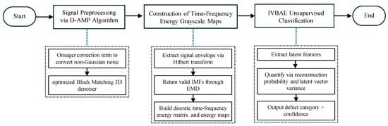
Figure 1. The flow chart of the proposed partial discharge pattern recognition method.

4. Results

To verify the effectiveness of the proposed method, this section first verifies the denoising effect of D-AMP using the simulated and measured PD UHF signals. Subsequently, the denoised UHF signals are further processed to generate time–frequency energy grayscale images. Finally, an improved variational Bayesian autoencoder is trained to verify its classification performance.

4.1. Experimental Data

The data used in this section includes simulated data and measured data. The simulated data are utilized to verify the effectiveness of the proposed signal denoising method, while the measured partial discharge data are utilized to verify the accuracy of the discharge pattern recognition. Simulated signals are generated based on a double-exponential decay oscillation model, which conforms to the radiation characteristics of GIS PD-UHF signals [36]. The model is presented as follows:

$$s(t)=G\cdot e^{-(t-t_0)/\tau }\cdot \sin [2\pi f(t-t_0)]\hspace{1em}(t\ge t_0)$$

(30)

where the sampling frequency is set to 20 GHz, the pulse amplitude G = 10, and the initial time $t_0$ = 2 ns. Two groups of differentiated signals are generated to cover different PD characteristics: typical signal 1 $\mathit{\tau }$ = 1.8 ns, f = 1.8 GHz; and typical signal 2 $\mathit{\tau }$ = 2 ns, f = 3.5 GHz.

To simulate the on-site interference environment, two types of typical noises are added to the simulated signals: Gaussian white noise and periodic narrowband interference (interference frequencies of 1.0 GHz and 1.5 GHz, and amplitudes of 3 and 5, synchronized with the 50 Hz power frequency). Two typical types of simulation signals are used to validate the denoising performance of the D-AMP method under controlled conditions. They are intended to reflect general PD signal characteristics, rather than to represent features associated with specific defect types.

Two typical types of simulation signals are denoted as typical signal 1 and typical signal 2. The waveforms of typical signal 1, both without and with noise, are presented in Figure 2a and Figure 2b, respectively. The corresponding spectra are shown in Figure 3. Similarly, the waveforms of typical signal 2 without and with noise are illustrated in Figure 4a and Figure 4b, respectively. The spectra are displayed in Figure 5.

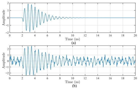
Figure 2. The waveform diagrams of PD UHF simulation signal 1: (a) the original noise-free signal; and (b) signal incorporated with Gaussian white noise and periodic narrowband interference.

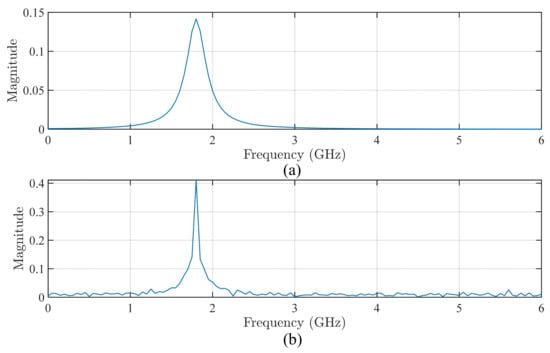
Figure 3. The spectra of signal 1: (a) the original signal; and (b) signal incorporated with the noises.

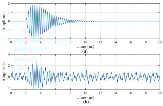
Figure 4. The waveform diagrams of PD UHF simulation signal 2: (a) the original noise-free signal; and (b) signal incorporated with Gaussian white noise and periodic narrowband interference.

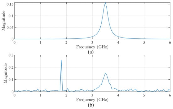
Figure 5. The spectra of signal 2: (a) the original signal; and (b) signal incorporated with the noises.

The measured signals are collected through a laboratory GIS defect simulation platform, including three typical defects: metal spikes, floating potentials, and free particles. Then, 200 valid samples are collected for each defect, totaling 600 samples for subsequent feature extraction and classification.

For UHF signal acquisition, a dual-sensor system was employed to accommodate different detection scenarios. The system consists of the following: (1) built-in integrated sensors (model: GM5010) are installed inside the GIS equipment, which are metal monopole antennae; and (2) external microstrip antenna sensors (model: PDDS102) are installed on the outer shell of GIS to detect radiated UHF electromagnetic waves. Signal acquisition was performed using a Keysight 6004 oscilloscope (manufactured by Keysight Technologies, Santa Rosa, CA, USA) with an analog bandwidth of 1 GHz and a sampling rate of 2.5 GSa.

The key antenna and probe characteristics are summarized as follows:

• Frequency response

The frequency response of both sensor types is measured using the time-domain reference method in a GTEM cell. Both sensors operate in the 300 MHz to 1500 MHz range, with equivalent heights of 10.68 mm for the GM5010 and 13.06 mm for the PDDS102.

2.

Voltage Standing Wave Ratio (VSWR)

The VSWR values were calculated from the scattering parameter S, which is calculated as follows:

$$\mathrm{VSWR}= \left(1+|\Gamma |\right)/\left(1-|\Gamma |\right)$$

(31)

where Γ is the reflection coefficient, $S= 20log\left|\Gamma \right|$.

For GM5010, $S_1$ = −6.33 dB ($\Gamma$ ≈ 0.48), corresponding to VSWR ≈ 2.85; for PDDS102, $S_{2 }$ = −2.35 dB ($\Gamma$ ≈ 0.74), corresponding to VSWR ≈ 6.69.

3.

Low-noise amplifier (LNA) matching

Each sensor is paired with a dedicated low-noise amplifier to preserve the signal integrity. The LNAs provide a noise figure of ≤2.5 dB and a gain of 35 dB across the operational frequency band.

4.2. The Verification of Signal Denoising Based on D-AMP

The improvement of the signal-to-noise ratio (ΔSNR) and mean square error (MSE) are used to quantify denoising effects. Among them, ΔSNR reflects the noise suppression capability, while MSE measures the deviation between the reconstructed signal and the original noise-free signal. Traditional denoising methods are selected as the control group, i.e., (i) wavelet transform [10] and (ii) singular value decomposition [12]. The denoising results under different noise scenarios are shown in Table 1.

Table 1. The denoising results of different denoising methods.

Noise Type	Method	ΔSNR (dB)	MSE (×10−3)
Gaussian Noise	WT	8.1	6.9
	SVD	6.5	7.2
	D-AMP	11.8	2.1
Narrowband Interference	WT	6.1	7.9
	SVD	8.5	6.2
	D-AMP	10.7	1.7
Gaussian + Narrowband Interference	WT	6.3	4.5
	SVD	7.8	3.1
	D-AMP	10.5	1.3

It can be found that, in Table 1, for the Gaussian noise, the ΔSNR of D-AMP reaches 11.8 dB, with an increase of 45.7% compared to WT (8.1 dB), and 38.8% compared to SVD (8.5 dB). The MSE of D-AMP is only 2.1 × 10⁻³, approximately one-third that of SVD, which greatly reduces the distortion of signals. For the narrowband interference, the ΔSNR of D-AMP is 10.7 dB, higher than that of WT (6.1 dB) and SVD (8.5 dB), and the MSE is reduced to 1.7 × 10−³. The simulation results demonstrated that the D-AMP could better retain the details of discharge pulses. For the Gaussian + narrowband mixed noise, the D-AMP still maintains a high ΔSNR of 10.5 dB, with the MSE as low as 1.3 × 10⁻³, which solves the problem of the insufficient adaptability of traditional methods in complex multi-noise scenarios. In summary, the D-AMP demonstrates a superior noise suppression and signal preservation performance over the traditional methods, such as WT and SVD.

The waveforms of the denoised typical signal 1 and typical signal 2 with the proposed method are shown in Figure 6, and their spectra are shown in Figure 7.

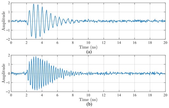
Figure 6. The waveforms of denoised signals: (a) signal 1; and (b) signal 2.

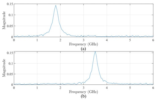
Figure 7. The spectra of denoised signals: (a) signal 1; and (b) signal 2.

Under the conditions of a well-designed measurement matrix and stable iteration, the Onsager correction term within D-AMP effectively approximates the non-Gaussian noise as Gaussian. This approximation aligns with the underlying assumption of the BM3D denoiser, which ensures consistency and coherence across the overall denoising framework. Meanwhile, the optimized BM3D effectively retains the rising edge and amplitude characteristics of PD pulses through the “time-domain DCT + pulse-dimensional wavelet” hybrid transform basis, avoiding the adaptability deficiency of traditional methods in multi-noise scenarios.

Under practical on-site measurement conditions, the original SNR of the measured PD UHF signals ranges from –5 dB to 0 dB, with a notable variation between sensor types. For built-in sensors, which are positioned closer to the PD source, the original SNR is comparatively higher (–2 dB to 0 dB), although the signals remain contaminated by significant background noise (amplitude ≈ 15 mV). In contrast, external sensors mounted at bushing insulator pouring ports exhibit a lower original SNR (–5 dB to –3 dB), where the weak PD pulses (amplitude ≈ 3 mV) are entirely buried in background noise.

Following denoising with the proposed D-AMP method, the SNR of the recovered PD signals improves substantially to 10 dB to 14 dB. The background noise amplitude is suppressed to below 1 mV, which enables the successful extraction of previously submerged PD pulses. Crucially, the essential characteristics of the pulses are preserved, thereby providing a reliable signal foundation for the subsequent time–frequency feature extraction and pattern-recognition analysis.

4.3. Time–Frequency Energy Feature Extraction Based on HHT

HHT is used for the time–frequency feature extraction and grayscale map conversion of denoised PD signals. First, EMD is used to extract IMF components; then, the Hilbert analysis is applied to generate three-dimensional time–frequency features; and, finally, to adapt to traditional deep learning models such as CNN, the three-dimensional time–frequency energy maps are converted into two-dimensional time–frequency energy grayscale maps. In this process, the time–frequency energy information in the original three-dimensional maps is completely retained, and the computational complexity is perfectly reduced.

Figure 8, Figure 9 and Figure 10 illustrate the time–frequency energy diagrams and two-dimensional grayscale images of the three types of partial discharge signals (metal spike, floating potential, and free particle).

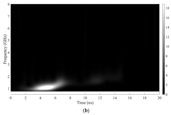
Figure 8. Metal spike partial discharge: (a) three-dimensional time–frequency energy distribution map; and (b) two-dimensional time–frequency energy grayscale map.

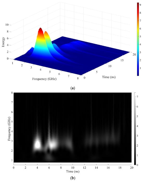
Figure 9. Floating potential partial discharge: (a) three-dimensional time–frequency energy distribution map; and (b) two-dimensional time–frequency energy grayscale map.

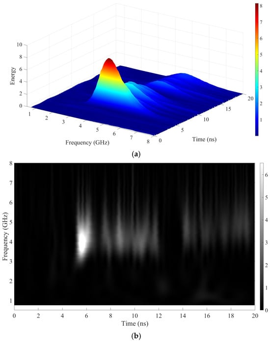
Figure 10. Free partial discharge: (a) three-dimensional time–frequency energy distribution map; and (b) two-dimensional time–frequency energy grayscale map.

In Figure 8, Figure 9 and Figure 10, metal spike defects exhibit continuous vertical energy stripes in the 0.8~1.2 GHz frequency band, corresponding to stable periodic discharges at the spike. Floating potential defects have periodic energy peaks distributed in the 1.0~1.5 GHz frequency band, with peak intervals consistent with the power frequency cycle. Free particle defects have scattered energy distribution, showing random dots in the 0.5~2.0 GHz range, corresponding to irregular discharges from particle collisions. This characteristic difference provides a clear basis for subsequent classification and avoids the limitation of traditional PRPD patterns relying on manual experience.

4.4. IVBAE Classification and Confidence Quantification

In this section, four types of traditional classification methods are selected as control groups, i.e., (i) Support Vector Machine [15] (SVM, combined with statistical features such as pulse amplitude and phase count), (ii) CNN [19], (iii) DBN [24], and (iv) traditional VAE [23]. All methods use the same dataset and optimizer parameters. Features for SVM and MLP are extracted using “non-zero mean” and “phase non-zero count”, while the inputs for CNN and IVBAE are HHT grayscale maps.

The confidence of PD pattern recognition is calculated with the probabilistic output of the improved VBAE. The measured data of three typical defects (metal spike, floating potential, and free particle) are used to verify the classification accuracy and confidence performance of the IVBAE model. In addition, the field noise is considered as a type of defect to further verify the classification accuracy, and the ratio of the training set, test set, and validation set for the above four types of data is 70%, 15%, and 15%, respectively. The statistics of the classification accuracy and confidence of the IVBAE model are shown in Table 2. It should be pointed out that the abbreviations used in Table 2 are explained as follows: Number of Test Samples (NTS), Number of Correct Classifications (NCC), Accuracy (Acc.), Number of High-Confidence Samples (NHCS), and Proportion of High-Confidence (PHC).

Table 2. Statistics of classification accuracy and confidence of the IVBAE model.

PD Pattern	NTS	NCC	Acc. (%)	NHCS	PHC (%)
Metal Spike	30	29	96.7	28	93.3
Floating Potential	30	28	93.3	26	86.7
Free Particle	30	27	90.0	25	83.3
Field Noise	30	28	93.3	28	93.3

In Table 2, the IVBAE achieves the highest recognition accuracy for metal spike defects (96.7%), followed by 93.3% for both the floating potential and field noise, and 90.0% for free particle defects. The average accuracy of IVBAE is 93.3%, which demonstrates the strong adaptability of the model to different defect types. Moreover, the average proportion of high-confidence samples is 87.8%, among which the proportion of high-confidence samples for the metal spike and field noise reaches 93.3%, indicating the extremely high reliability of the model for defect samples with clear features. Even for free particle defects with scattered features, the proportion of high-confidence samples is 83.3%, which also verifies the effectiveness of the IVBAE model.

To quantify the accuracy of different PD pattern recognition methods, the following indicators are utilized, i.e., Accuracy, Precision, Recall, and F1-score. Their formulae are shown below:

$$\mathrm{Accuracy}={\displaystyle \frac{TP+TN}{TP+TN+FP+FN}}$$

(32)

$$\mathrm{Precision}={\displaystyle \frac{TP}{TP+FP}}$$

(33)

$$\mathrm{Recall}={\displaystyle \frac{TP}{TP+FN}}$$

(34)

$$\mathrm{F}1\text{-}\mathrm{score}=2\times {\displaystyle \frac{\mathit{Precision}\times \mathit{Recall}}{\mathit{Precision}+\mathit{Recall}}}$$

(35)

where TP is the number of correctly classified positive samples, TN is the number of correctly classified negative samples, FP is the number of negative samples incorrectly classified as positive, and FN is the number of positive samples incorrectly classified as negative [37].

The comparison of the accuracy of different PD mode recognition methods is shown in Table 3.

Table 3. Comparison of the accuracy of different PD mode recognition methods.

Method	Metal Spike (%)	Floating Potential (%)	Free Particle (%)	Average (%)	Mean F1-Score
SVM	76.7	73.3	66.7	72.2	0.720
CNN (LeNet-5)	86.7	83.3	76.7	83.3	0.821
DBN (3 layers)	86.7	85.0	78.3	83.9	0.838
VAE	90.0	86.7	81.7	86.1	0.859
IVBAE	96.7	93.3	90.0	93.3	0.931

Furthermore, to intuitively present the classification performance and misclassification distribution characteristics of different pattern recognition methods, Figure 11 shows the comparison of the classification confusion matrices of five algorithms for three typical PD defects.

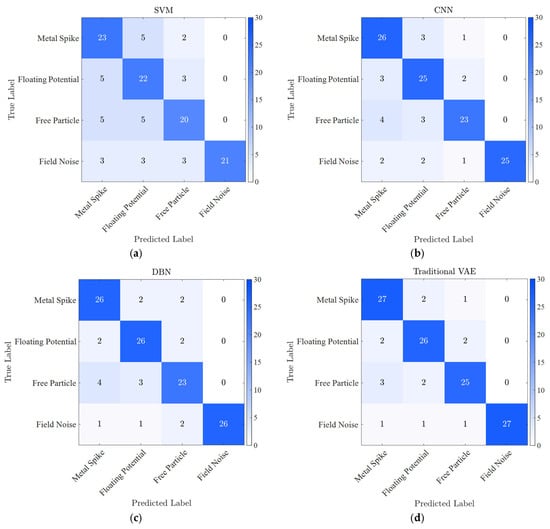
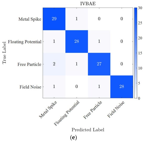
Figure 11. Comparison of classification confusion matrices of different pattern recognition methods for typical PD defects and field noise in GIS: (a) SVM; (b) CNN; (c) DBN; (d) Traditional VAE; and (e) IVBAE.

It can be found that, in Table 3, the SVM achieves an average classification accuracy of 72.2%, with the free particle defects only reaching 66.7%, accompanied by severe misclassifications. The CNN and DBN have average accuracies of 82.2% and 83.9%, respectively, where the free particle defects still suffer from considerable misclassifications. The traditional VAE improves the average accuracy to 86.1%, with reduced misclassifications but insufficient adaptability to multimodal data.

Moreover, in Table 3 and Figure 11, the IVBAE achieves an average accuracy of 93.3%, exceeding the traditional VAE, CNN, and SVM by 8.4%, 13.5%, and 29.2%, respectively. The recognition accuracy for free particle defects reaches 90.0%, 13.3% higher than that of CNNs, which solves the problem of the poor classification effect of traditional methods on defects with scattered features. The accuracy for metal spike defects reaches 96.7% with no false positive samples. The results demonstrate the strong feature discrimination capability. The average F1-score of IVBAE reaches 0.931, much higher than other methods, indicating that it achieves a good balance between precision and recall, and the classification results are more robust.

5. Conclusions

This paper proposes a novel method for the PD pattern recognition of GIS that integrates D-AMP denoising, HHT time–frequency feature representation, and IVBAE recognition. It effectively addresses the key issues of the existing methods, such as the poor denoising adaptability in complex noise scenarios, excessive reliance on expert experience, and lack of reliability verification for classification results.

Experimental results show that the D-AMP denoising method exhibits a strong robustness in multi-noise scenarios. Compared with traditional methods such as WT and SVD, the proposed method achieves a substantially higher improvement in ΔSNR. The time–frequency energy grayscale map can clearly distinguish the features among different typical defects, providing reliable feature support for subsequent classification. The IVBAE model designed with GM latent space and patch convolution achieves an average classification accuracy of 93.3%, which is significantly better than traditional methods such as the SVM, CNN, and VAE. Meanwhile, the model realizes the quantification of classification confidence through a comprehensive uncertainty index, solving the “black-box decision-making” problem of traditional artificial intelligence methods. The proposed method improves the accuracy and reliability of the online diagnosis of GIS insulation defects, which supports the stable operation of power systems.

References

- Zhang, G.; Tian, J.; Zhang, X.; Liu, J.; Lu, C. A Flexible Planarized Biconical Antenna for Partial Discharge Detection in Gas-Insulated Switchgear. IEEE Antennas Wirel. Propag. Lett. 2022, 21, 2432–2436. [Google Scholar] [CrossRef]
- Shu, Z.; Wang, W.; Yang, C.; Guo, Y.; Ji, J.; Yang, Y.; Shi, T.; Zhao, Z.; Zheng, Y. External Partial Discharge Detection of Gas-Insulated Switchgears Using a Low-Noise and Enhanced-Sensitivity UHF Sensor Module. IEEE Trans. Instrum. Meas. 2023, 72, 1–10. [Google Scholar] [CrossRef]
- Partyka, M.; Bridges, G.E.; Kordi, B. Online Partial Discharge Measurements in an Operating Generator Stator Winding Using Uhf Antennas. IEEE Trans. Dielectr. Electr. Insul. 2023, 31, 1593–1602. [Google Scholar] [CrossRef]
- Kong, X.; Zhang, C.; Hou, C.; Lin, X.; Du, B. UHF Sensor for Partial Discharge Detection Based on Coplanar Waveguide Feeding. IEEE Sens. J. 2024, 24, 28119–28128. [Google Scholar] [CrossRef]
- Kameli, S.M.; Refaat, S.S.; Abu-Rub, H.; Darwish, A.; Ghrayeb, A.; Olesz, M. Ultrawideband Vivaldi Antenna with an Integrated Noise-Rejecting Parasitic Notch Filter for Online Partial Discharge Detection. IEEE Trans. Instrum. Meas. 2024, 73, 1–10. [Google Scholar] [CrossRef]
- Chang, C.S.; Jin, J.; Chang, C.; Hoshino, T.; Hanai, M.; Kobayashi, N. Separation of Corona Using Wavelet Packet Transform and Neural Network for Detection of Partial Discharge in Gas-Insulated Substations. IEEE Trans. Power Deliv. 2005, 20, 1363–1369. [Google Scholar] [CrossRef]
- Raghavendra, B.; Chaitanya, M.K. Comparative Analysis and Optimal Wavelet Selection of Partial Discharge De-Noising Methods in Gas-Insulated Substation. In Proceedings of the 2017 Third International Conference on Advances in Electrical, Electronics, Information, Communication and Bio-Informatics (AEEICB), Chennai, India, 27–28 February 2017; pp. 1–5. [Google Scholar]
- Satish, L.; Nazneen, B. Wavelet-Based Denoising of Partial Discharge Signals Buried in Excessive Noise and Interference. IEEE Trans. Dielectr. Electr. Insul. 2003, 10, 354–367. [Google Scholar] [CrossRef]
- Zhongrong, X.; Ju, T.; Caixin, S. Application of Complex Wavelet Transform to Suppress White Noise in GIS UHF PD Signals. IEEE Trans. Power Deliv. 2007, 22, 1498–1504. [Google Scholar] [CrossRef]
- Huang, N.E.; Shen, Z.; Long, S.R.; Wu, M.C.; Shih, H.H.; Zheng, Q.; Yen, N.-C.; Tung, C.C.; Liu, H.H. The Empirical Mode Decomposition and the Hilbert Spectrum for Nonlinear and Non-Stationary Time Series Analysis. Proc. R. Soc. Lond. A 1998, 454, 903–995. [Google Scholar] [CrossRef]
- Chan, J.C.; Ma, H.; Saha, T.K.; Ekanayake, C. Self-Adaptive Partial Discharge Signal de-Noising Based on Ensemble Empirical Mode Decomposition and Automatic Morphological Thresholding. IEEE Trans. Dielectr. Electr. Insul. 2014, 21, 294–303. [Google Scholar] [CrossRef]
- Zhong, J.; Bi, X.; Shu, Q.; Chen, M.; Zhou, D.; Zhang, D. Partial Discharge Signal Denoising Based on Singular Value Decomposition and Empirical Wavelet Transform. IEEE Trans. Instrum. Meas. 2020, 69, 8866–8873. [Google Scholar] [CrossRef]
- Ashtiani, M.B.; Shahrtash, S.M. Partial Discharge De-Noising Employing Adaptive Singular Value Decomposition. IEEE Trans. Dielectr. Electr. Insul. 2014, 21, 775–782. [Google Scholar] [CrossRef]
- Li, X.; Ding, D.; Xu, Y.; Jiang, J.; Chen, X.; Yuan, M. A Denoising Method for Partial Discharge Ultrasonic Signals in GIS Based on Ultra-High Frequency Signal Synchronization. IEEE Trans. Power Deliv. 2024, 39, 3316–3325. [Google Scholar] [CrossRef]
- Gao, W.; Ding, D.; Liu, W. Research on the Typical Partial Discharge Using the UHF Detection Method for GIS. IEEE Trans. Power Deliv. 2011, 26, 2621–2629. [Google Scholar] [CrossRef]
- Zhang, S.; Li, C.; Wang, K.; Li, J.; Liao, R.; Zhou, T.; Zhang, Y. Improving Recognition Accuracy of Partial Discharge Patterns by Image-Oriented Feature Extraction and Selection Technique. IEEE Trans. Dielectr. Electr. Insul. 2016, 23, 1076–1087. [Google Scholar] [CrossRef]
- Kunicki, M.; Cichoń, A. Application of a Phase Resolved Partial Discharge Pattern Analysis for Acoustic Emission Method in High Voltage Insulation Systems Diagnostics. Arch. Acoust. 2018, 43, 235–243. [Google Scholar] [CrossRef]
- Zhang, X.; Xiao, S.; Shu, N.; Tang, J.; Li, W. GIS Partial Discharge Pattern Recognition Based on the Chaos Theory. IEEE Trans. Dielectr. Electr. Insul. 2014, 21, 783–790. [Google Scholar] [CrossRef]
- Song, H.; Dai, J.; Sheng, G.; Jiang, X. GIS Partial Discharge Pattern Recognition via Deep Convolutional Neural Network under Complex Data Source. IEEE Trans. Dielectr. Electr. Insul. 2018, 25, 678–685. [Google Scholar] [CrossRef]
- Peng, X.; Yang, F.; Wang, G.; Wu, Y.; Li, L.; Li, Z.; Bhatti, A.A.; Zhou, C.; Hepburn, D.M.; Reid, A.J. A Convolutional Neural Network-Based Deep Learning Methodology for Recognition of Partial Discharge Patterns from High-Voltage Cables. IEEE Trans. Power Deliv. 2019, 34, 1460–1469. [Google Scholar] [CrossRef]
- Zhang, C.; Chen, M.; Zhang, Y.; Deng, W.; Gong, Y.; Zhang, D. Partial Discharge Pattern Recognition Algorithm of Overhead Covered Conductors Based on Feature Optimization and Bidirectional LSTM-GRU. IET Gener. Transm. Distrib. 2024, 18, 680–693. [Google Scholar] [CrossRef]
- Nguyen, M.-T.; Nguyen, V.-H.; Yun, S.-J.; Kim, Y.-H. Recurrent Neural Network for Partial Discharge Diagnosis in Gas-Insulated Switchgear. Energies 2018, 11, 1202. [Google Scholar] [CrossRef]
- Lu, S.; Chai, H.; Sahoo, A.; Phung, B.T. Condition Monitoring Based on Partial Discharge Diagnostics Using Machine Learning Methods: A Comprehensive State-of-the-Art Review. IEEE Trans. Dielectr. Electr. Insul. 2020, 27, 1861–1888. [Google Scholar] [CrossRef]
- Chen, Y.; Zhao, X.; Jia, X. Spectral–Spatial Classification of Hyperspectral Data Based on Deep Belief Network. IEEE J. Sel. Top. Appl. Earth Obs. Remote Sens. 2015, 8, 2381–2392. [Google Scholar] [CrossRef]
- Li, G.; Rong, M.; Wang, X.; Li, X.; Li, Y. Partial Discharge Patterns Recognition with Deep Convolutional Neural Networks. In Proceedings of the 2016 International Conference on Condition Monitoring and Diagnosis (CMD), Xi’an, China, 25–28 September 2016; pp. 324–327. [Google Scholar]
- Chen, J.; Xu, C.; Li, P.; Shao, X.J.; Li, C.L. Feature Extraction Method for Partial Discharge Pattern in GIS Based on Time-Frequency Analysis and Fractal Theory. High Volt. Eng. 2021, 47, 287–295. [Google Scholar]
- Metzler, C.A.; Maleki, A.; Baraniuk, R.G. From Denoising to Compressed Sensing. IEEE Trans. Inf. Theory 2016, 62, 5117–5144. [Google Scholar] [CrossRef]
- Yuan, Y.; Huang, Z.; Wu, H.; Wang, X. Specific Emitter Identification Based on Hilbert–Huang Transform-based Time–Frequency–Energy Distribution Features. IET Commun. 2014, 8, 2404–2412. [Google Scholar] [CrossRef]
- Dang, N.-Q.; Ho, T.-T.; Vo-Nguyen, T.-D.; Youn, Y.-W.; Choi, H.-S.; Kim, Y.-H. Supervised Contrastive Learning for Fault Diagnosis Based on Phase-Resolved Partial Discharge in Gas-Insulated Switchgear. Energies 2023, 17, 4. [Google Scholar] [CrossRef]
- Song, S.; Qian, Y.; Wang, H.; Zang, Y.; Sheng, G.; Jiang, X. Partial Discharge Pattern Recognition Based on 3D Graphs of Phase Resolved Pulse Sequence. Energies 2020, 13, 4103. [Google Scholar] [CrossRef]
- Zemouri, R.; Levesque, M.; Amyot, N.; Hudon, C.; Kokoko, O.; Tahan, S.A. Deep Convolutional Variational Autoencoder as a 2d-Visualization Tool for Partial Discharge Source Classification in Hydrogenerators. IEEE Access 2019, 8, 5438–5454. [Google Scholar] [CrossRef]
- Thi, N.-D.T.; Do, T.-D.; Jung, J.-R.; Jo, H.; Kim, Y.-H. Anomaly Detection for Partial Discharge in Gas-Insulated Switchgears Using Autoencoder. IEEE Access 2020, 8, 152248–152257. [Google Scholar] [CrossRef]
- Ganjun, W.; Fan, Y.; Xiaosheng, P.; Yijiang, W.; Taiwei, L.; Zibo, L. Partial Discharge Pattern Recognition of High Voltage Cables Based on the Stacked Denoising Autoencoder Method. In Proceedings of the 2018 International Conference on Power System Technology (POWERCON), Guangzhou, China, 6–8 November 2018; pp. 3778–3792. [Google Scholar]
- Li, Y.; Yang, J.; Cui, Z.; Wang, C.; Gao, T.; Liu, S.; Shu, Z. A Few Shot Partial Discharge Diagnosis Method Based on Dual-Path Variational Autoencoder. In Proceedings of the 2025 IEEE 8th International Electrical and Energy Conference (CIEEC), Changsha, China, 16–18 May 2025; pp. 887–892. [Google Scholar]
- Jing, Q.; Yan, J.; Wang, Y. A Novel Partial Discharge Pattern Recognition for GIS with Unbalanced Sample Based on Conditional Variational Autoencoder. In Proceedings of the 18th International Conference on AC and DC Power Transmission (ACDC 2022), Online, 2–3 July 2022; IET: London, UK, 2022; Volume 2022, pp. 1314–1319. [Google Scholar]
- Huijuan, H.; Gehao, S.; Wenjuan, J. Signal Reconstruction for Partial Discharge Electromagnetic Wave in Substation Based on Signal Model Parameters Identification. High Volt. Eng. 2015, 41, 209–216. [Google Scholar] [CrossRef]
- Li, A.; Wei, G.; Li, S.; Zhang, J.; Zhang, C. Pattern Recognition of Partial Discharge in High-Voltage Cables Using TFMT Model. IEEE Trans. Power Deliv. 2024, 39, 3326–3337. [Google Scholar] [CrossRef]
Disclaimer/Publisher’s Note: The statements, opinions and data contained in all publications are solely those of the individual author(s) and contributor(s) and not of MDPI and/or the editor(s). MDPI and/or the editor(s) disclaim responsibility for any injury to people or property resulting from any ideas, methods, instructions or products referred to in the content. |
© 2025 by the authors. Licensee MDPI, Basel, Switzerland. This article is an open access article distributed under the terms and conditions of the Creative Commons Attribution (CC BY) license.