Abstract
Energy generated from wind (in the form of wind farms (WFs)) is expected to help alleviate rising energy demand in Saudi Arabia, driven by industrial development and population growth. However, before implementing wind farms, conducting a comprehensive wind resource assessment (WRA) study is of paramount importance. This paper presents the analysis of the wind resource potential of a site in Yanbu city, which is located on the western coastal area of Saudi Arabia, using a comprehensive study. The hourly data on wind speed and direction over a one-year period was used in the presented analysis. The plant capacity factor (CF) and annual energy production (AEP) are evaluated for more than 100 commercial wind turbines (WTs). The highest AEP was achieved by the ‘Enercon E126/7.5 MW’ turbine, generating 14.49 GWh, with a corresponding CF of 21.82%. In contrast, the lowest AEP was observed for the ‘Northern Power d’ turbine, producing only 0.13 GWh, with a CF of 14.89%. The highest CF was recorded for the ‘Leitwind LTW104/2.0 MW’ turbine at 40.67%, corresponding to an AEP of 7.12 GWh. The results obtained are very valuable for designers in selecting the appropriate WT to obtain the predicted AEP and CF with the appropriate turbine class. Furthermore, this study applied the K-means clustering algorithm to classify WTs into three distinct categories. Building on this classification, synthetic datasets representing tailored WT configurations were generated—a novel methodology that enables the simulation of site-specific designs not yet available in existing market offerings. These datasets equip wind farm developers with the ability to define WT specifications for manufacturers, guided by two key criteria: the site’s wind resource profile and the target performance metrics of the WT.
1. Introduction
The wind power market and industry have grown substantially in the last decade, marked by the significant increase of wind power installed capacity around the globe [1]. REN21 reported that in 2020, more than 86.9 GW of onshore wind power was installed, with offshore wind power at nearly 6.1 GW. The global total capacity increased 45% as compared to 2015 installations [2]. The significant progress of wind energy development has been achieved through strong implementation plans and policies and supported by declining wind energy costs over the last decade [3]. Therefore, it is expected that wind energy development will expand rapidly in the coming year, as the global wind power market continues to grow.
Wind Resource Assessment (WRA) is a critical first step in Wind Farm (WF) development, as it directly influences both initial investment costs and long-term economic viability. The precision of these evaluations plays a decisive role in determining energy production potential and financial returns throughout the project’s lifecycle [4,5,6]. WRA has been carried out using various methods in multiple countries and different regions. Dong et al. [7] investigated wind power resources by simulating a wind field near the Yangtze River Delta using a Weather Research Forecasting model. Simulated data for a 35-year period were used to calculate the spatial distribution of the average wind speed in monthly and annual time scales, with the wind energy rose simulated at six different locations. Zhang et al. [8] developed a platform that can be used to assess wind energy resources in Shandong province in the East of China based on data mining. Tri-level assessment is applied by firstly analyzing, processing, and correcting the long-term meteorological data. At the next two levels, the dimensionality is reduced, and the temporal and spatial synergy patterns are captured using data mining techniques. Such a framework is useful to plan renewable energy sources. In another study [9], a long-term WRA was conducted for the South China Sea based on 30-year hindcast data. The results show that offshore winds are comparably stronger than nearby regions, with average annual energy densities reaching up to 1100 W/m2. The potential of wind resources was investigated in Ukraine using 30-min time scale data for a period of eight years [10]. In this investigation, probabilistic analysis techniques were applied to derive the temporal variations of wind speed and direction. In comparison with the data for the other two periods, the temporal changeability was determined. Chandel et al. [11] assessed wind resource potential for decentralized power generation in the western Himalayan region using wind speed data measured at several intervals and different hub heights. It was found that shorter time intervals give a larger mean power density.
A feasibility study of wind resources for utility-scale wind power development was conducted using Wind Atlas Analysis and Application Program (WAsP 12.1) software for the selected locations in Fiji [12]. The wind resources were simulated and analyzed based on wind speed and direction, power density, and energy production. Wind resource data maps were produced for three recommended sites, with an average wind speed of 7 m/s or greater, which is generally considered commercially viable for utility-scale wind power. Saeed et al. [13] investigated the feasibility of wind resources at eighteen different sites in Pakistan using the Kolmogorov–Smirnov statistic-based optimization method with Weibull distribution. The assessment was conducted to evaluate whether the available wind resources are technically feasible and economically viable based on average power density and Levelized Cost of Energy (LCOE). In another study [14], the Kolmogorov–Smirnov method combined with the Wilcoxon–Mann–Whitney method was used to assess large-scale wind resource features in Algeria, and wind speed characteristics were analyzed using Generalized Extreme Value (GEV) distribution. Wan et al. [15] used Weibull distribution to model the wind speed, and the Cross-Entropy (CE) method was introduced to estimate the parameters. The measurement data of four wind towers were used to evaluate six wind energy metrics. It was found that this method is superior for assessing wind energy resources in Urat, Mongolia.
An assessment of wind energy potential was performed in India based on a Geographical Information System (GIS) using multi-year meteorological data sets [16]. The techno-economic feasibility results indicate that the western region has the highest renewable energy potential, at around 3.1 TW wind energy availability and 1.15 $/kWh LCOE. Auktino et al. [17] investigated the wind energy resource potential in Kiribati using ambient temperature and pressure, wind speed, and direction data measured at two locations. WAsP software was used to analyze wind resource maps, and assessment of wind energy potential was conducted based on Annual Energy Production (AEP) and economic analysis for both locations. A feasibility study for applying wind energy in Cameroon was conducted by Kazet et al. [18]. In this study, a small WF comprising four 1.65 MW Wind Turbines (WTs) was investigated in terms of AEP using 1-year data of climate, topography, and roughness. The results were compared to WAsP analysis for high wind resource areas. In other studies, WAsP analysis was also used to assess wind energy resources in the Fiji Islands [19] and in Sinai Peninsula, Egypt, as combined with WindPro software [20]. Charabi et al. [21] investigated wind energy application in Oman for several selected potential sites using two numerical weather prediction models, i.e., HRM and COSMO. The weak local wind circulation was simulated to evaluate the models’ ability, and wind power output was calculated to assess wind energy resources. Ayik et al. [22] conducted a preliminary WRA and statistical analysis for 33 locations in South Sudan using reanalysis data for the period between 1981 and 2019. In another study, an assessment of wind energy potential was conducted using reanalysis data for the east coast of India [23]. The analysis results using longer-duration datasets such as one year were sufficiently close to the available measured data. Energy system deployment and the development of offshore wind energy resource maps were evaluated for the coastal regions of Africa using satellite-based remote sensing systems [24]. In this assessment, a 6 h dataset of wind speed from 2001 to 2011 was used to identify potential sites for wind turbine installation. The offshore wind resources were analyzed at different heights, considering variation of seasonal climate conditions in different regions of Africa. In a recent study, Neupane et al. [25] proposed a spatial energy model using the GIS platform. Technical, geographical, and economic suitability criteria were applied to investigate solar and wind energy potential in Nepal. The model is useful in formulating energy policies for the country.
In recent years, numerous research works and applications have been used to accelerate the implementation of WFs through carrying out investigation of wind resource potential. WRA has been conducted using various models and methods to assess wind energy feasibility. For example, a polynomial regression model as the probability density function for wind speed frequency was used to overcome the shortcomings of the distribution models at lower wind speed [26]. In another study, the combination of GIS and multi-criteria decision making was used for analysis of potential locations for wind energy development [27]. For this purpose, resource variability was explored and forecasted using the Adaptive Neuro-Fuzzy Inference System (ANFIS) to improve strategic and operational planning. New equations developed by Galvez et al. [28] were used to assess the wind resource feasibility for three sites in Mexico based on mesoscale and microscale models. Sensitivity analysis of the LCOE was conducted in low-wind-potential sites to investigate the feasibility of wind resources under certain market conditions. Silvera et al. [29] developed wind and solar resource assessment and prediction using Artificial Neural Network (ANN) and semi-empirical models for the Colombian Caribbean region. In this study, statistical analysis was performed based on meteorological data. In a recent study in 2021 [30], Elshafei et al. proposed a hybrid solution for offshore WRA from limited onshore measurements as a critical pre-construction of WFs. This approach is a combination of the intermittent measurement and the continuous simulation data for the assessment of the west coast of Denmark. An ANN was then used to conduct spatial data fusion for the projection of onshore wind to offshore locations.
The present research aims to investigate the feasibility of wind energy resources for WT installation and operation. A comprehensive WRA approach is proposed and applied to a potential site in the city of Yanbu, Saudi Arabia. In this study, wind speed and direction are analyzed to find pattern and, trends and to select the direction of the WT to be placed in the WF. For implementation purposes, more than 100 commercial WTs were investigated and tested to determine the AEP and Capacity Factor (CF) of the selected site. Moreover, the results of this study will be valuable for accelerating the wind energy development, not only for Saudi Arabia but also for other countries.
The main contributions of this paper can be summarized as follows:
Extensive evaluation of commercial wind turbines: Unlike most studies that analyze a small selection of wind turbines, our work evaluates over 100 commercial WTs, providing a broader perspective on turbine selection for the specific site in Yanbu.
Application of K-means clustering for turbine classification: While WRA studies typically classify turbines based on predefined categories, we apply unsupervised machine learning (K-means clustering) to categorize turbines objectively based on their AEP and CF, offering a data-driven classification approach. To the best of our knowledge this application is investigated for the first time in our paper.
Introduction of synthetic wind turbine data generation: A key novelty of this study is the generation of synthetic WT configurations, allowing WF developers to explore new WT specifications tailored to the site’s wind characteristics. To the best of our knowledge this application is investigated for the first time in our paper.
Future-oriented contribution to wind energy development: Our findings not only assist in current turbine selection but also propose a framework for future turbine design by manufacturers, linking WRA with practical industry applications.
2. Wind Resource Assessment Approach
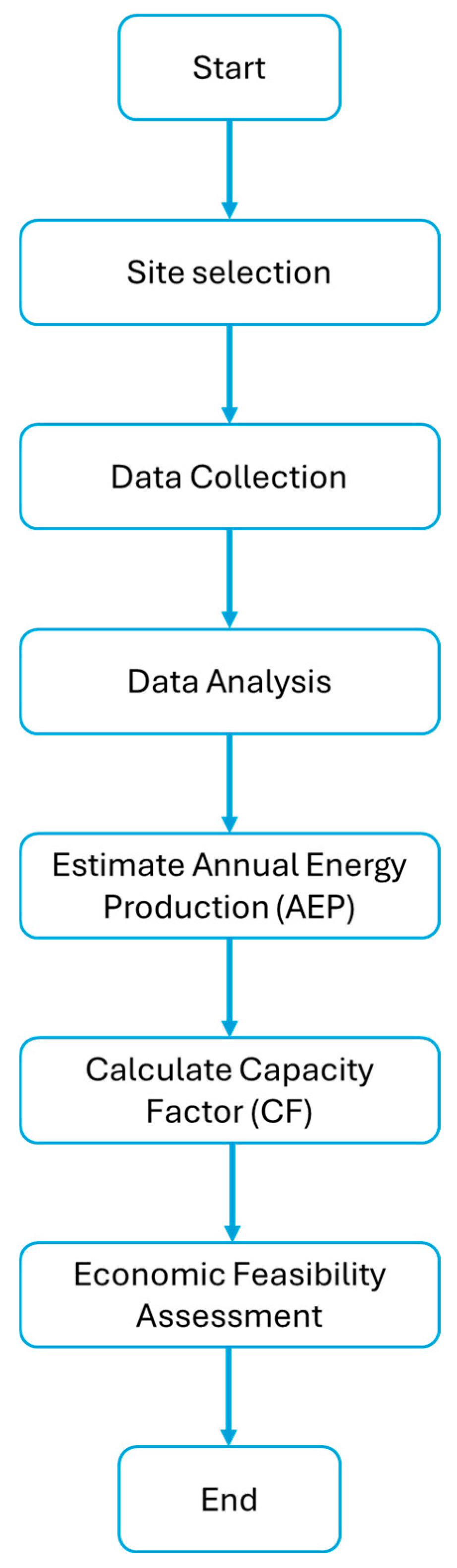
WRA aims to estimate the amount of energy that can be generated by a wind power plant or a WF over a given lifetime of the WT [31]. This activity includes the process of measurement and analysis of meteorological and wind speed data at a specific location [32]. To determine the economic feasibility of a wind project, the AEP is the most important quantity to be estimated in addition to the CF. In this study, a comprehensive WRA approach is proposed as shown in Figure 1. It starts with the selection of the right potential site and ends with the estimation of the AEP and plant CF.
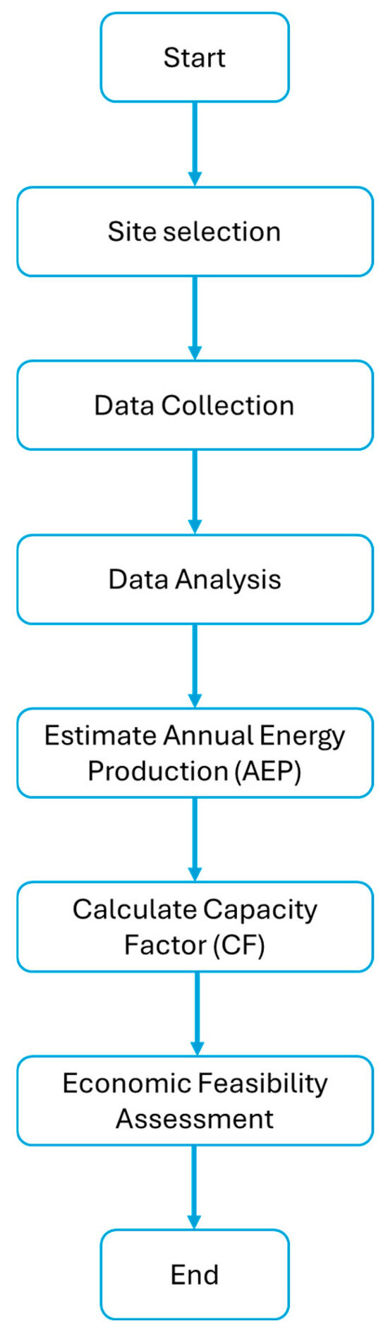
Figure 1.
The proposed WRA approach.
2.1. Site Selection
One of the most important conditions for the success of wind project design and development is the selection of potential sites. This selection is mainly based on the available wind resources for the site along with the location of the load centers with respect to the site, transmission access, market conditions and regulations, and public support [31].
2.2. Analysis of Measured Time Series Wind Data
The first step in a WRA investigation, after selecting a potential site, is to gather sufficient data for analysis. As reported in [31], the data of at least 1 year are needed. Once the data are collected from metrological centers, these data are deeply analyzed. The objective is to identify any trend or patterns in the data that can guide the remaining study.
2.3. Data Quality Assurance
Like many measurement datasets, wind data often contain missing values or gaps due to various factors. These gaps can result from inaccurate data recording, transmission failures, network congestion, or issues with data-collecting devices. Additionally, factors like low aerosol concentrations or unwanted fixed echoes in remote sensing devices can further impact data quality. Adverse weather conditions, such as thunderstorms, may also contribute to data loss, along with problems related to sensors, data loggers, or power supplies. Such low-quality data can significantly degrade the accuracy and completeness of the dataset, ultimately harming the effectiveness of the remaining steps of the WRA approach [33,34,35].
In the proposed WRA approach, the initial step involves conducting quality assurance tests on the data. If any data fail to meet the quality standards due to missing values or gaps, a couple of options can be considered:
- The first option consists of replacing the failed data using a variety of methods, from simple interpolation techniques to complex Artificial Intelligence (AI)-based models. This approach can incorporate historical data from similar sites to enhance accuracy.
- The second option consists of removing the failed data from the dataset.
In our application, we choose option 2. This means we will remove the failed data, focusing our analysis solely on the data that successfully passe all quality assurance tests. This approach ensures that our subsequent analyses are based on high-quality, reliable data.
2.4. Wind Speed Distribution
Two probability density functions given by Equations (1) and (2) are usually used to describe the wind speed distribution [31,36,37]. The first one, called the Rayleigh distribution, requires only the wind speed to calculate the probability density function, whilst the second one, called the Weibull distribution, requires two parameters, which are the shape parameter, referred to as and the scale parameter, referred to as . The Weibull probability density function is used in this study.
where is the wind speed and is the mean wind speed.
Estimating Weibull Probability Density Function Parameters
The Weibull probability density function is widely used to characterize wind speed and to estimate power density for WF projects [31]. One of the methods for estimating the Weibull parameters is the maximum likelihood. In this method, which is recommended by many researchers, the parameter is determined using an iteration-based process, whilst the parameter is solved explicitly, as expressed by Equations (3) and (4), respectively [31].
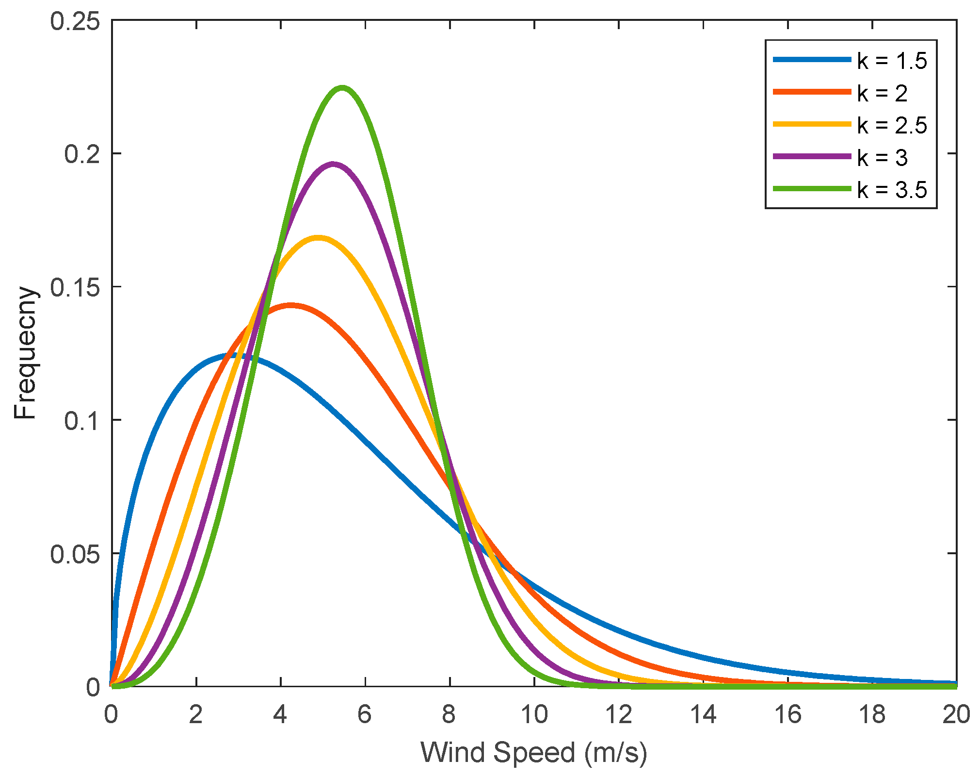
As reported in [36], the unitless parameter is often around 2. This value can be used as a good starting point for the iterative process to determine a more accurate value of . In fact, the Rayleigh distribution given by Equation (1) is a special case of the Weibull distribution, with . Furthermore, Figure 2 shows an illustration of the effect of the shape parameter on the Weibull distribution with scale parameter . It is worth mentioning that a higher value of indicates a more consistent wind speed, with most data points clustering around the mean. Conversely, a lower value of indicates greater variability in wind speed.
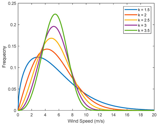
Figure 2.
Illustration of Weibull distributions with and different values for .
2.5. Wind Speed Variability
Variation of wind direction is also important in WF development projects. Knowing and identifying the wind direction is very important for the assessment of wind and the control of WT. The characteristics of wind speed and direction can be analyzed using the wind rose plot. It shows the frequency distribution of wind direction in a polar form.
In addition to wind rose plots, daily and monthly curves of wind speed at different heights are evaluated in this step to determine any possible pattern or trend or the period of most wind.
2.6. Wind Shear Profile
As reported in [31] most of the wind measuring sensors and devices are at 10 m elevation. However, most of WTs are installed at heights superior to 10 m. The wind speed at any height based on measurements at a given height can be calculated using a logarithmic function or power function, as given in the following equations [31,38,39]:
where is the wind speed at height , is the wind speed at height , is the roughness exponent, and is the roughness length.
In this study, the power function is used to determine the wind speed at a given hub height based on the measurements obtained at another reference height. The shape of this power function depends on the roughness exponent . Some typical values of for different terrain types are given below [40].
- -
- Smooth: 0.1
- -
- Untilled ground or short grass: 0.14
- -
- Few buildings and many trees: 0.22–0.24
- -
- Urban area: 0.4
Furthermore, Prandtl suggested a value of 1/7 [41]. The International Electrochemical Commission (IEC) supposes for design calculation [42]. However, wind shear at a given site cannot be just one value, since it is affected by many factors, as reported in [36,43]. In this study is used, as recommended by the IEC.
In some cases, more than one sensor is installed at the same location, with each sensor placed at a different height. In such cases, the data obtained can be used to extrapolate the value of wind speed at the desired hub height.
2.7. Turbulence Intensity
Studying the turbulence intensity for a WF is very important. It helps to estimate many factors, like the load of different components, the fatigue of equipment, WT control, and the power output [31]. The turbulence intensity, referred to as , is defined as the ratio of the standard deviation () over the average speed measured () during a period, and it is expressed as follows [31,32]:
The can be affected by different factors, like daytime, season, hub height, wind direction, and wind speed. However, the IEC has established a model to determine the based on the wind speed, and it is expressed as follows [42]:
where and are two parameters that depend on the class of the WT used in the site. WT classes are explained in detail in the next section.
As aforementioned, one of the most important factors influencing the turbine’s dynamics is the turbulence of the wind acting on it. High turbulence can significantly impact the fatigue loading on wind turbines, ultimately affecting their lifespan. Although turbulence is an environmental factor that cannot be controlled, it is crucial to understand its effect on turbine fatigue. This knowledge is essential for the design process to ensure the turbine structure can withstand increased turbulence levels. For turbines located in regions with stable wind speeds, the design requirements can be less stringent. However, in areas subject to high turbulence, wind gusts, or extreme phenomena like typhoons, the designer must account for the severe turbulence and its impact on the dynamic loading of the turbine structure. Additional details about the effect of turbulence intensity on the fatigue lifetime of wind turbines are given in [44].
2.8. Wind Turbine Class
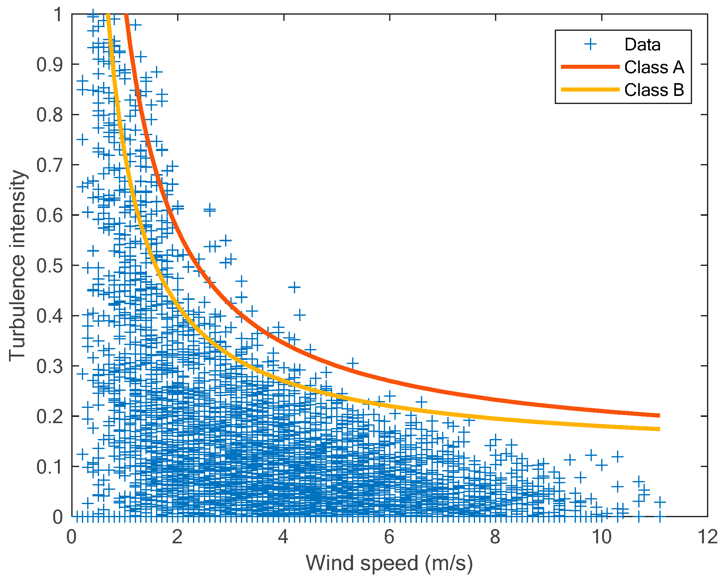
IEC classifies WTs into four classes based on the average wind speed and turbulence intensity [34]. For instance, Siemens SWT-2.3-108, a class IIB wind turbine, is designed for medium wind and low turbulence intensity, whilst the Siemens SWT-2.3-93, a class IIA wind turbine, is designed for medium wind and high turbulence intensity. Therefore, the class for WTs should be appropriate for the selected site of WF.
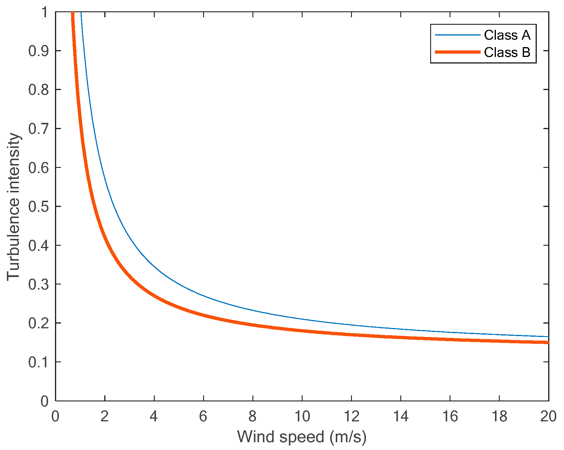
Using the values given in IEC 61400-1 [42] for class A and class B wind turbines, we can plot the turbulence intensity , as shown in Figure 3.

Figure 3.
IEC design turbulence intensities for class A and class B.
2.9. Wind Turbine Power Curve
WTs convert the wind kinetic energy into mechanical power, which can be used to drive mechanical components to generate electricity [31]. The power density of wind allows us to determine the amount of power that can be generated using a specific WT. The power curve refers to the power output of a wind turbine that is related to wind speed [32]. The output power depends mainly on three factors: wind speed, air density, referred to as and the size of the WT (represented by which is the area of the rotor). The power density available in the wind neglecting losses can be expressed as follows [31]:
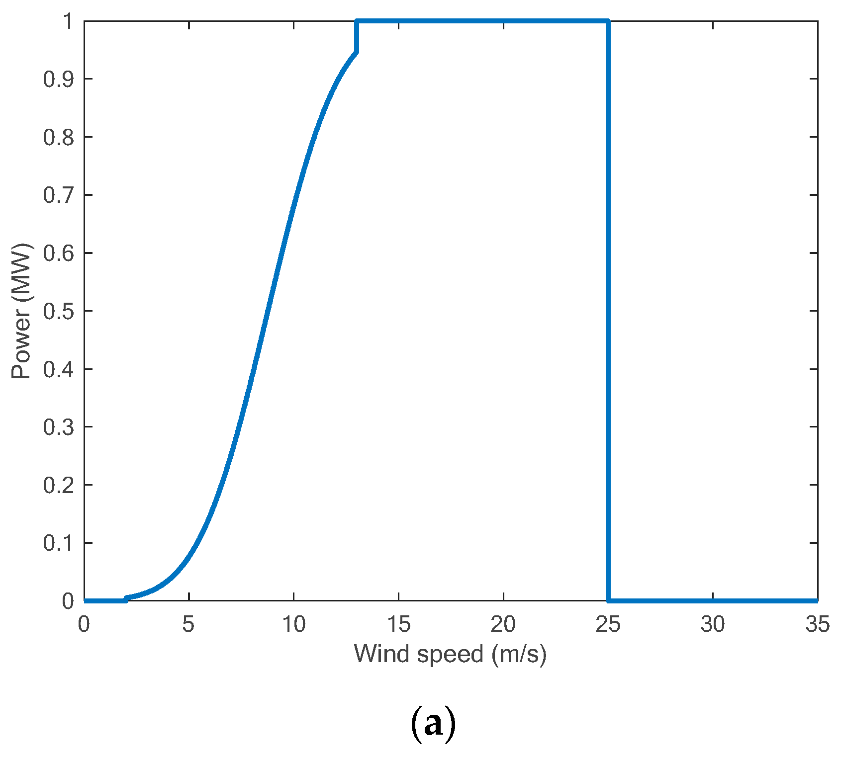
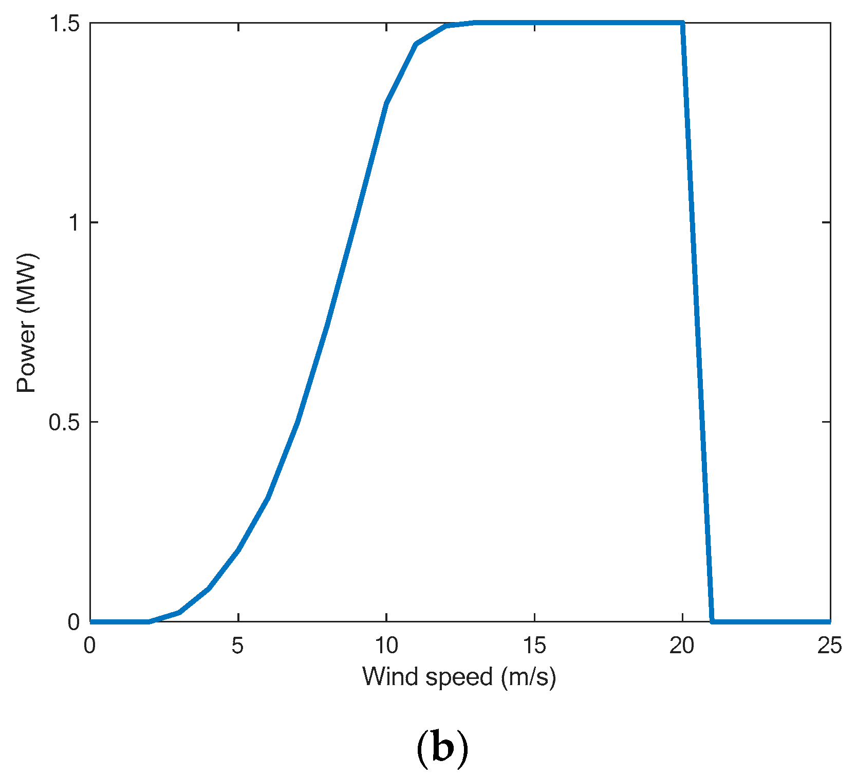
Figure 4a shows an illustration of a power curve for a WT that has the following characteristics: , , , and . It can be observed from Figure 4b that below the cut-in speed, there is no output power because the WT does not operate due to small torque, which is not sufficient to rotate the blades. If the wind speed increases, the WT starts to generate power until it reaches the rated speed and power. However, if the speed increases above the cut-out speed, the WT is shut down for safety reasons and therefore there is no output power.
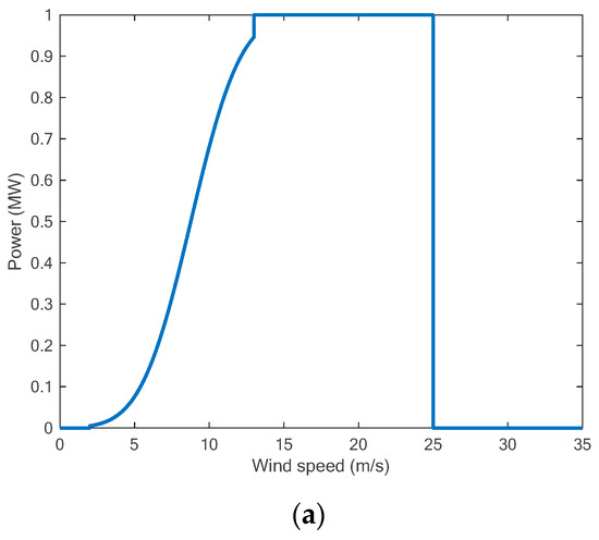
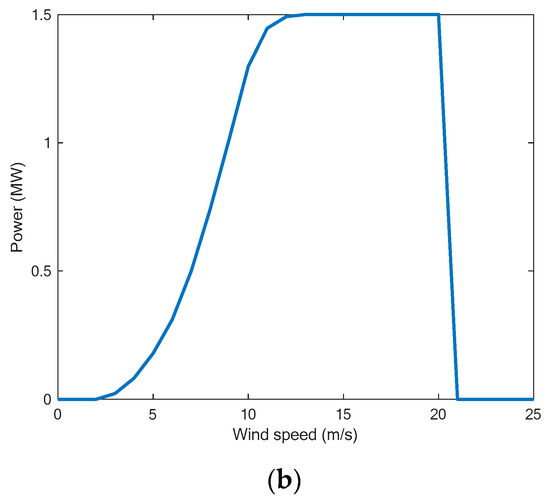
Figure 4.
(a) Example of a WT power curve. (b) Real power curve for the ‘Acciona AW82/1500 kW’ WT.
A real power curve obtained from [45] for the ‘Acciona AW82/1500 kW’ class IIIB WT is depicted in Figure 4b.
2.10. Wind Direction Variability and Its Affect on Power
Nearly all modern wind turbines are designed to align with the incoming wind direction through both yaw and pitch control systems. The yaw system adjusts the nacelle to align with the prevailing wind direction, while the pitch control system constantly modifies the angle of attack of the rotor blades to optimize energy capture. However, wind direction variability can have a significant impact on turbine performance, leading to reduced energy production and increased wear on mechanical components. Misalignment due to fluctuating wind directions can also shorten the lifespan of turbines. Therefore, accurately modeling wind direction variability and understanding the effects of yaw misalignment are crucial for designing more efficient yaw control systems and improving WF flow controllers, ultimately leading to better overall performance and reliability [46,47]. While this paper does not focus on this topic, we provide here just a brief overview of how wind direction variability can impact the power output of wind turbines. For a more comprehensive analysis, please refer to [46,47].
A WT that experiences yaw misalignment exhibits a decrease in power generation. This power sensitivity to yaw misalignment can be quantified by the power–yaw loss exponent as follows [46,47]:
where is the yaw misalignment angle between the turbine rotor and the local wind direction, as shown in Figure 5. is the power generated by a wind turbine with a yaw misalignment of . is the power generated when the turbine experiences no yaw misalignment. The term is referred to as the Power Reduction Factor (PRF).
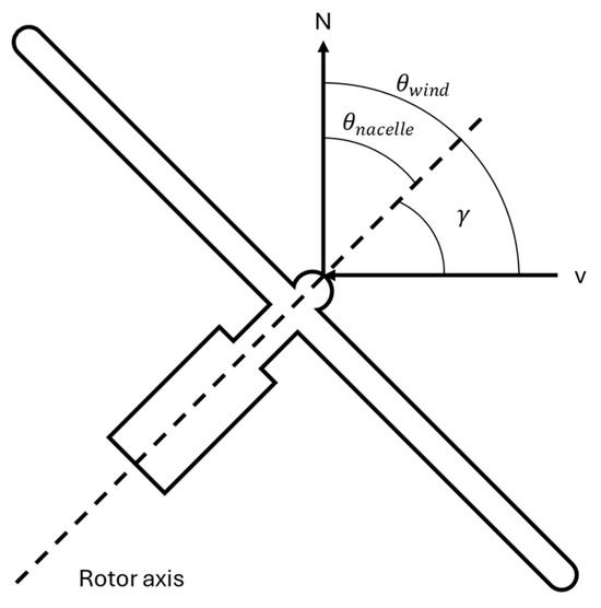
Figure 5.
Illustration of the yaw misalignment on a horizontal axis WT [46].
2.11. Annual Energy Production
As aforementioned, the WRA is the first preliminary task in a WF development project, with the goal of determining the available power (or energy) density of the project site. The power (or energy) density represents the power (or energy) available in the project site per area and per unit time. The AEP helps WF designers and project engineers to estimate the total Annual Energy (AE) that can be extracted from the project site. Therefore, estimating the AEP is one of the main goals for wind resource assessment for a WF project. The AEP is a crucial factor that will determine the financial viability of a WF project. It is estimated by using wind data available at the project site along with the power curve of a tested WT.
The energy produced by a given WT using continuous or discrete data can be determined using the following expressions.
For continuous data [32],
For discrete data [32],
where is the wind speed measured over time, and is the curve of power output based on the wind speed.
However, in practice, these expressions may be infeasible, and another approach is used based on sorting the wind speed data into histograms, multiplying the frequencies and the power curve , and then estimating the energy by taking the sum of this product. For continuous data, the expression of the energy is given by [32]
For discrete data, the expression of the energy can be expressed as follows [32]:
Finally, the AEP, which is defined as the total annual energy generated over a period of 1 year by a given WT measured in (kWh) or (MWh), can be determined using the following expression [32]:
2.12. Capacity Factor
The capacity factor, referred to as is very important in determining the performance of a WF project. It is calculated using the following equation [32]:
where Prated is the rated power of WT, and ET is the actual energy output per year.
As reported in [32], the generally ranges between 20% and 40%, and obtaining a greater than 30% is the target. It is worth mentioning that a low value of may indicate that the WF project is not viable because the wind resources are not good or the WT is oversized.
2.13. Wind Farm Site Selection Factors
A critical step before developing the technical project is identifying the most suitable location for the WF. Site selection for WFs involves a comprehensive assessment of multiple factors. Various elements need to be considered, and several of these are thoroughly discussed and investigated in [48]. The location should be at least 500 m away from the main road network and 1000 to 3000 m from urban areas. The land’s slope must be less than 15°. Additionally, the plant’s elevation should not exceed 2000 m, as higher altitudes result in reduced air density, which can lead to lower turbine efficiency. WFs should also be situated at a safe distance from transmission lines, mining operations, protected areas, historical heritage sites, military zones (at least 5000 m from radar installations), forests, railways, ecological corridors, wildlife habitats, migration routes, and watercourses. Lastly, areas prone to natural disasters—such as cyclones, hurricanes, landslides, floods, storms, and tornadoes—should be avoided in the site selection process. More details can be found in [48].
3. Application and Results
3.1. Site Selection
The site selected to be assessed in this study is Yanbu city, which has the following geographical parameters: Latitude: 24.144722; Longitude: 38.063611; and Elevation: 18.0 m a.s.l.
Yanbu is a port city located at the western coast of Saudi Arabia; it is only 6 m above the sea level [49]. Furthermore, it is the second largest industrial city after Jubail in the country. Yanbu is an excellent site for WF project assessment and evaluation. The wind map for this city is displayed in [39]. Like other cities in Saudi Arabia, this city has two seasons, i.e., summer (between the months of March and September) and winter (between the months of October and February) [49].
3.2. Analysis of Measured Time Series Wind Data
For this study, data with a high resolution of 250 m for the full year of 2013 were collected from SolarGIS [50]. The data are organized as follows:
- -
- Date of measurement;
- -
- Time of measurement with a time step of 60 min;
- -
- Global horizontal irradiation [Wh/m2];
- -
- Direct normal irradiation [Wh/m2];
- -
- Diffuse horizontal irradiation [Wh/m2];
- -
- Sun altitude (elevation) angle [deg.];
- -
- Sun azimuth angle [deg.];
- -
- Air temperature at 2 m [°C];
- -
- Atmospheric pressure [hPa];
- -
- Relative humidity [%];
- -
- Wind speed at 10 m [m/s];
- -
- Wind direction [deg.].
It is important to note that while a variety of meteorological and environmental data were available, not all were utilized in this study. In particular, solar-related data were not explored, as the focus of this research was solely on wind resource assessment and wind turbine evaluation. These additional data types may be considered in future studies to support hybrid renewable energy system analysis.
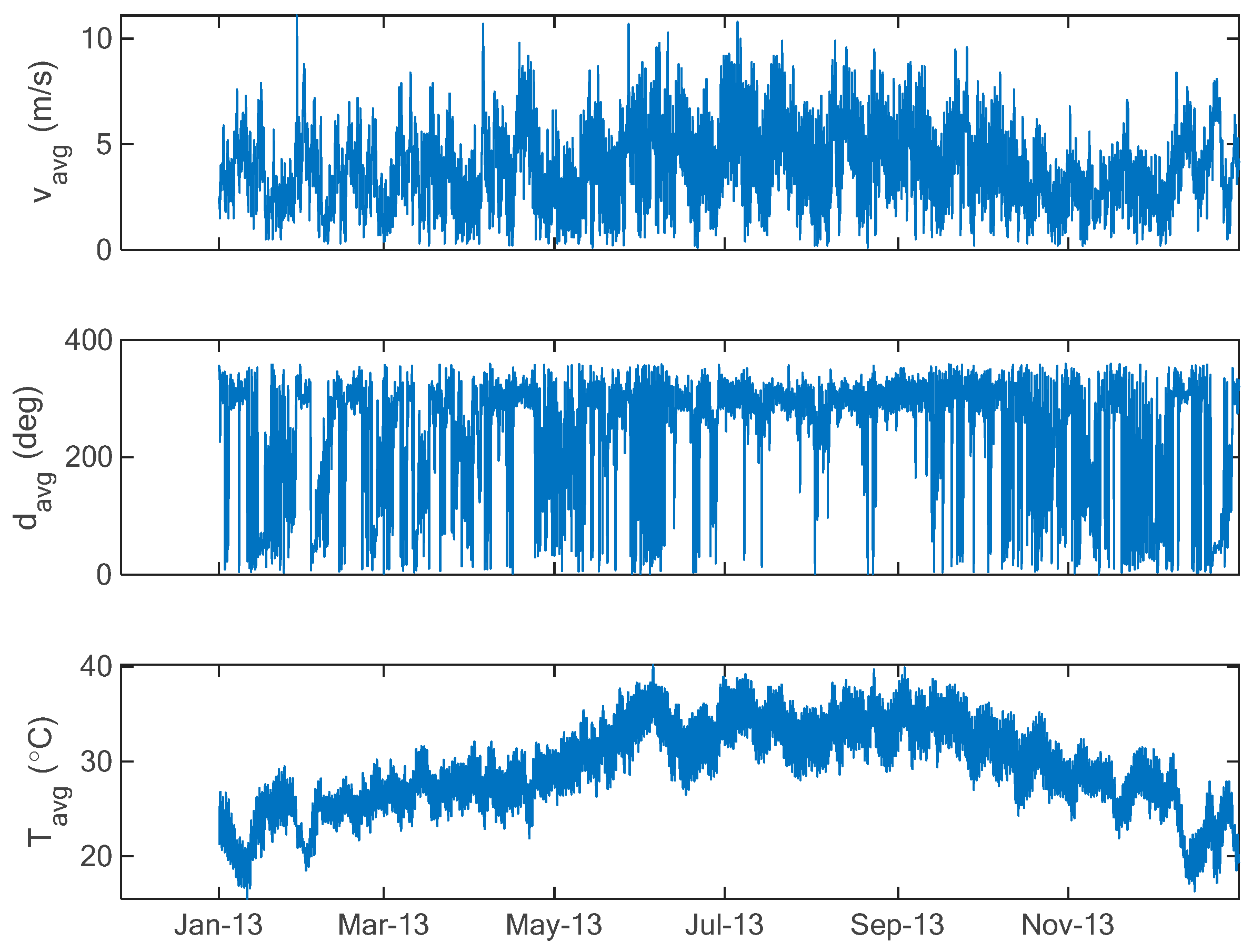
First, the raw data are presented in Figure 6. The first curve represents the hourly average speed in (m/s) at 10 m, the second curve represents the hourly average wind direction measured in (deg), whilst the last curve represents the air temperature at 2 m in (°C) as measured in Yanbu city at the selected location.
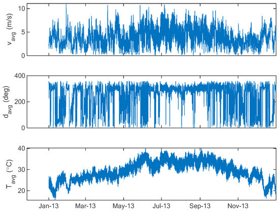
Figure 6.
Hourly data measured at Yanbu city for year 2013.
3.3. Data Quality Assurance
The data used were checked, and no abnormal or missing values were found.
3.4. Wind Speed Distribution
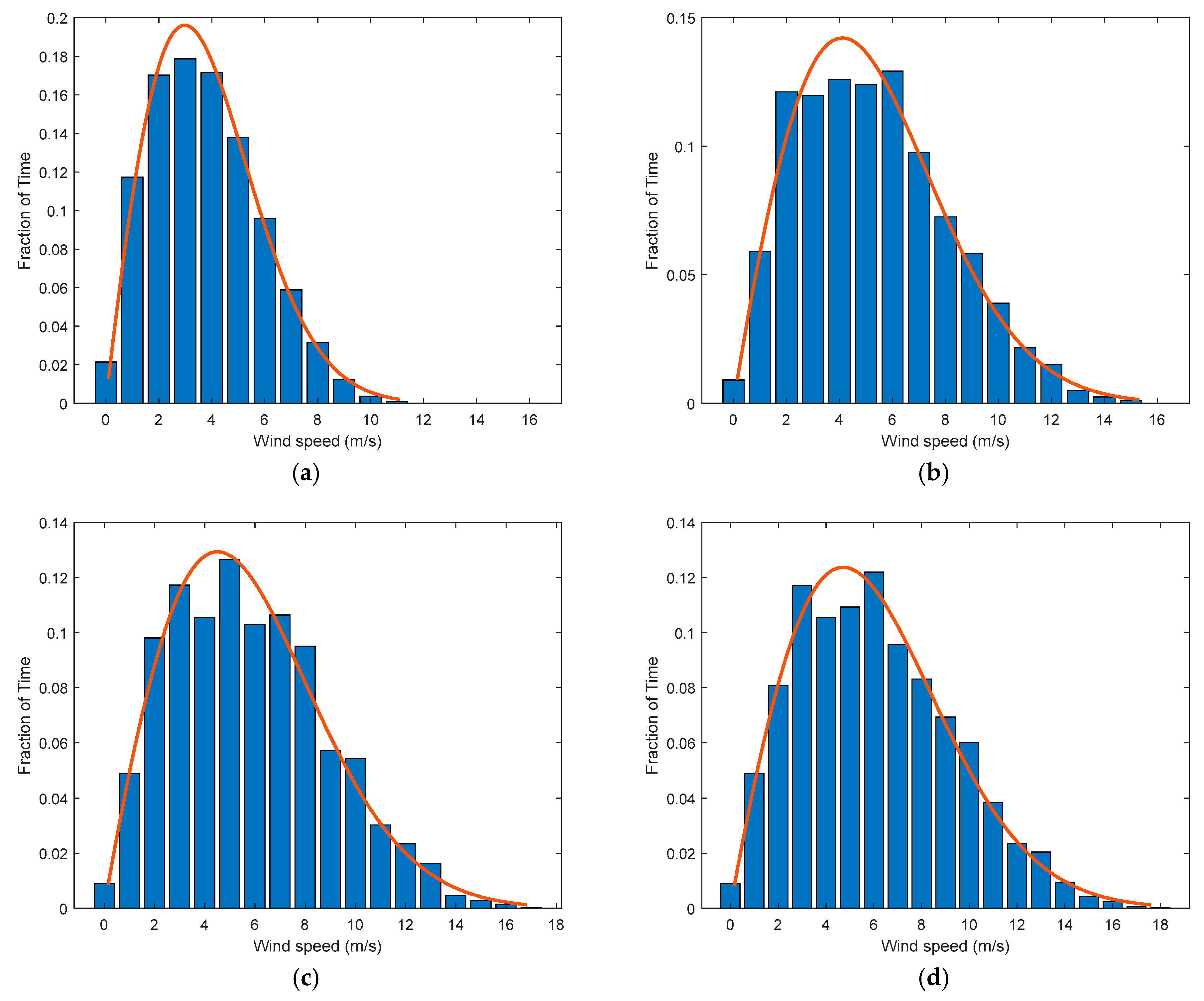
The wind distribution at the measurement height (i.e., at 10 m) and at different hub heights (i.e., at 50 m, 80 m, and 100 m) is plotted in Figure 7. Furthermore, the Weibull distribution function explained in Section 2.4 was fitted using the maximum likelihood method; the parameters (the estimated parameters along with 95% confidence interval for the estimates) are given, and the fitted curve is sketched on the measured values, as shown in Figure 7. It can be observed from Figure 7 that the Weibull curve fits the real wind speed data. The estimated shape factor is 1.95. This value falls within the common values of k in Saudi Arabia, between 1.95 and 2.60, as reported in [51].
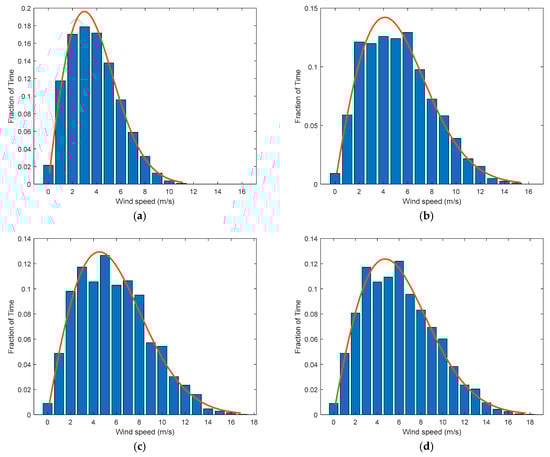
Figure 7.
Wind speed histogram with Weibull fit at Yanbu.
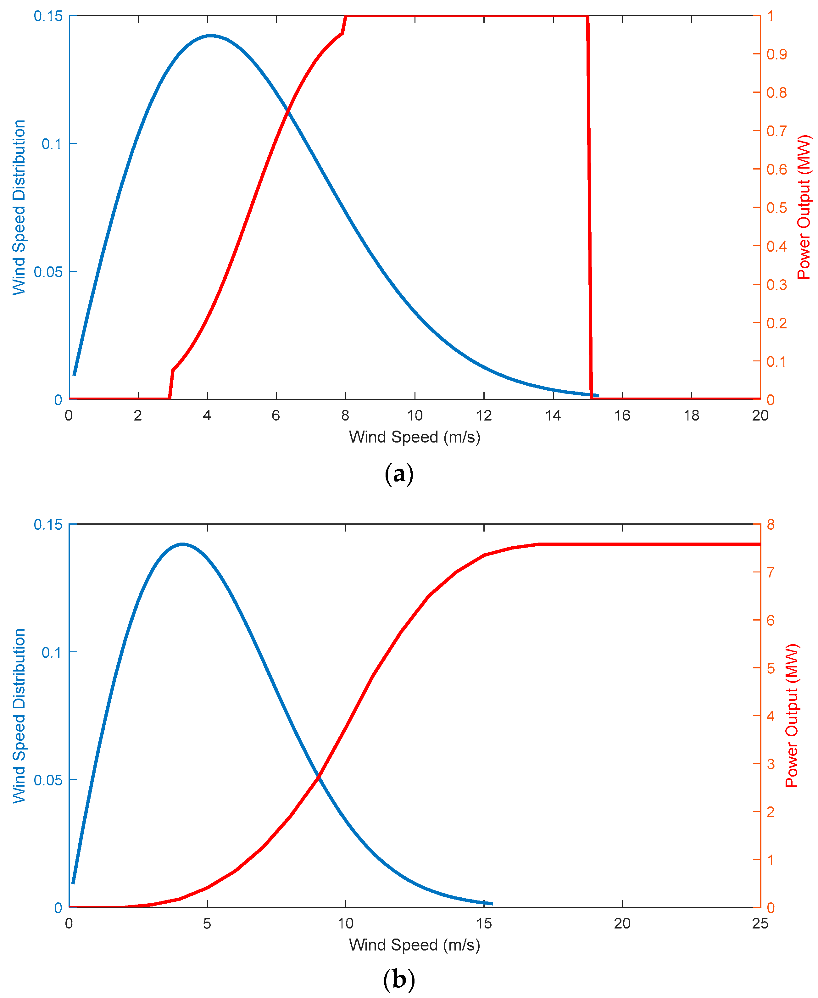
3.5. Power Curve and Wind Distribution
To predict the wind production, the distribution, and not a single point, is needed. An illustration of the wind speed distribution and power output for two commercial WTs is shown in Figure 8.
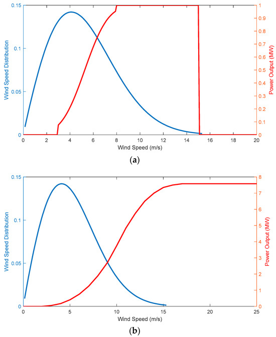
Figure 8.
Example of a WT power curve along with wind speed distribution for the (a) ‘Acciona AW82/1500 kW’ and (b) ‘Enercon E126/7.5 MW’ WTs.
3.6. Wind Speed Variability
3.6.1. Wind Rose
Figure 9 shows the wind rose plot obtained for the data measured at 10 m for Yanbu city. It can be observed from this figure that wind is dominant and prevailing from the northwest around 30% of the time at 320°. On the opposite side, the wind blows slightly from southeast (less than 5%), with a speed less than 0.5 m/s. Therefore, the WTs to be installed must face the northeast, as demonstrated by the wind rose plot.
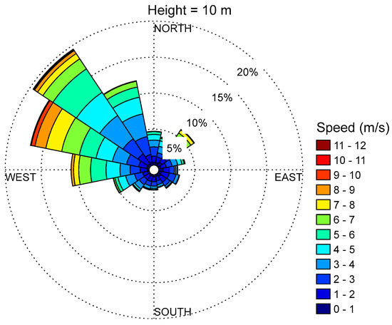
Figure 9.
Wind rose plots at Yanbu.
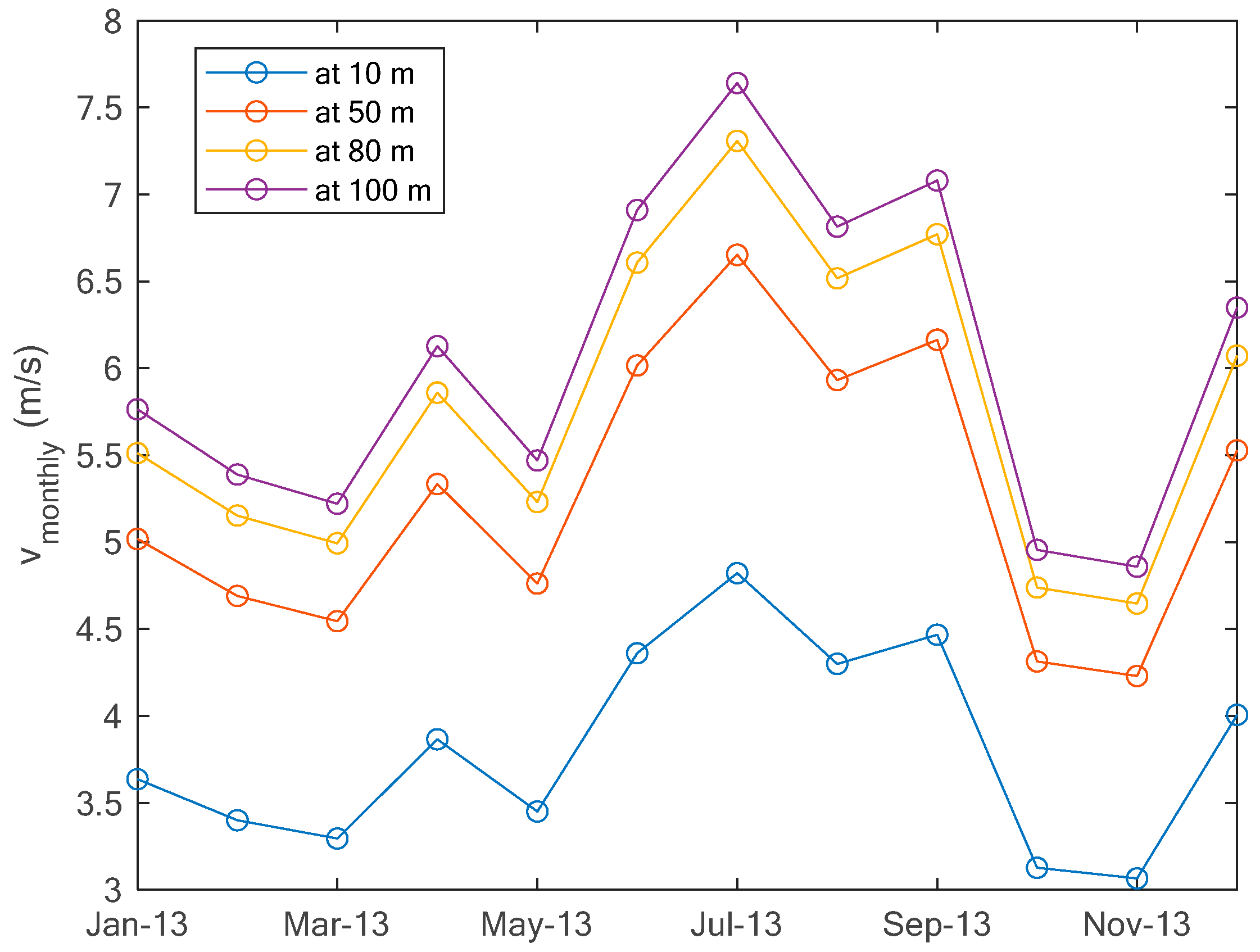
3.6.2. Monthly Average Wind Speeds
The monthly average wind speeds measured at 10 m and those calculated at hub heights (i.e., at 50 m, 80 m, and 100 m) are given in Figure 10. The wind speeds at hub height are higher than those at 10 m, as expected. It can be observed also that the wind speed is more important in the summer season from June to September than the remaining year. The peaks in monthly wind speeds for measured and calculated speeds are observed in July, with wind speeds of 4.822 m/s, 6.653 m/s, 7.308 m/s, and 7.642 m/s, whilst the minimums are observed in November, with wind speeds of 3.066 m/s, 4.230 m/s, 4.647 m/s, and 4.859 m/s.

Figure 10.
Monthly average wind speeds at Yanbu.
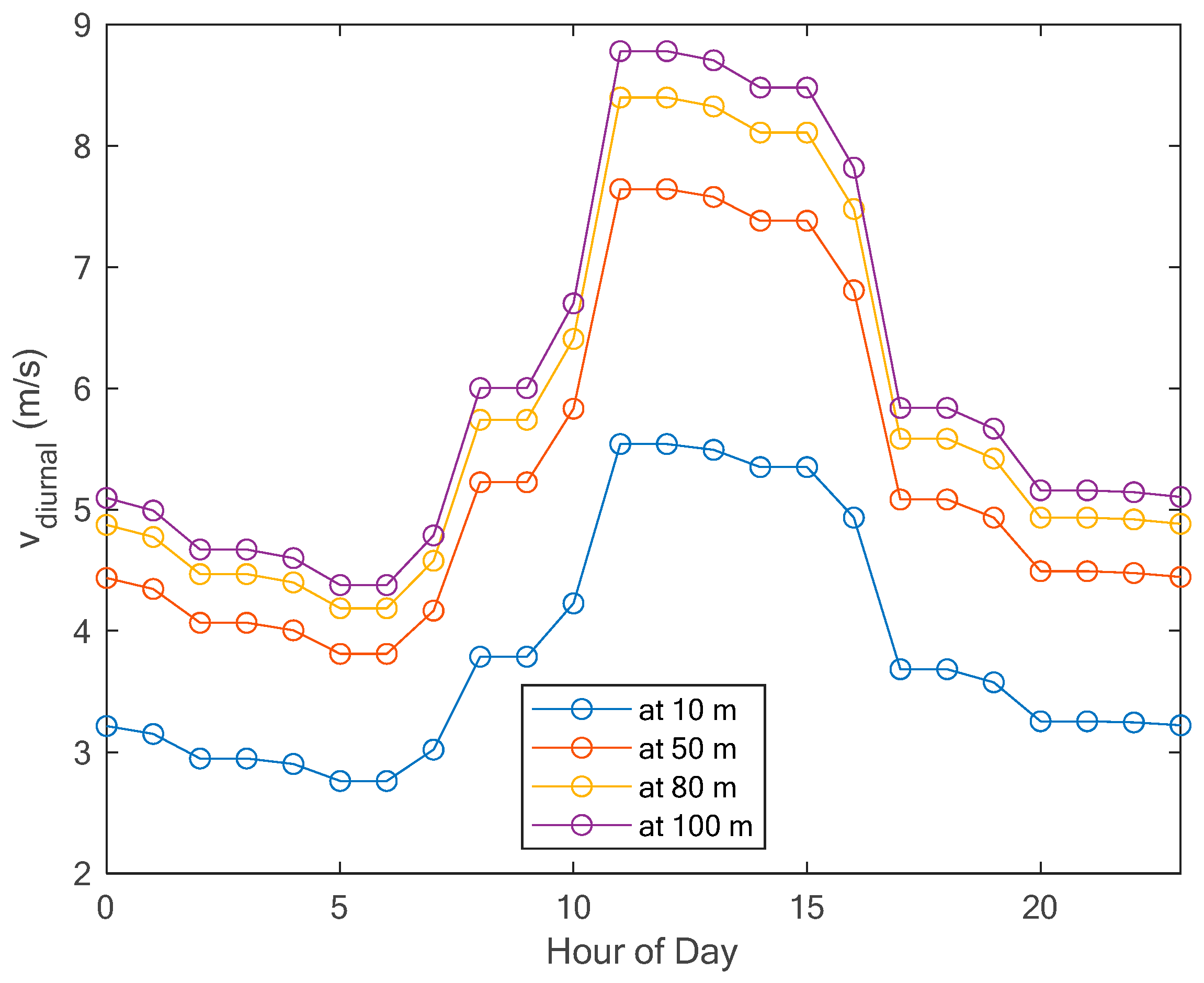
3.6.3. Diurnal Average Wind Speeds
Diurnal average wind speeds measured at 10 m and those calculated at hub heights (i.e., at 50 m, 80 m, and 100 m) are shown in Figure 11. As expected, wind speeds at hub height are higher than those at 10 m. It can be observed also from Figure 11 that wind blows more from 11:00 a.m. to 4:00 p.m., with a speed around 5 m/s at 10 m hub height, around 7.5 m/s at 50 m hub height, around 8.3 m/s at 80 m hub height, and around 8.6 m/s at 100 m hub height.
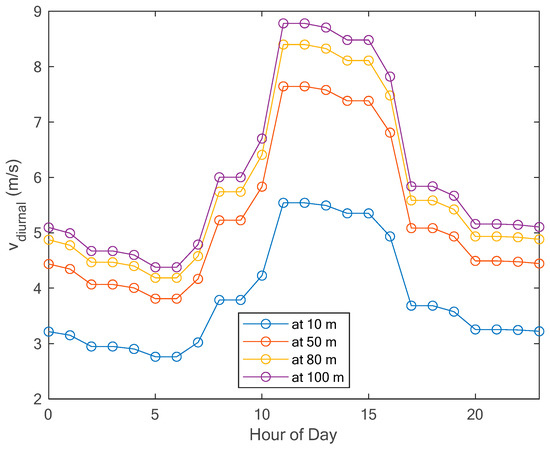
Figure 11.
Diurnal average wind speeds at Yanbu.
3.7. Turbulence Intensity
The turbulence intensity was estimated using Equation (7) for each 1 h interval and is plotted in Figure 12 with respect to the average speed.

Figure 12.
Turbulence intensity at Yanbu.
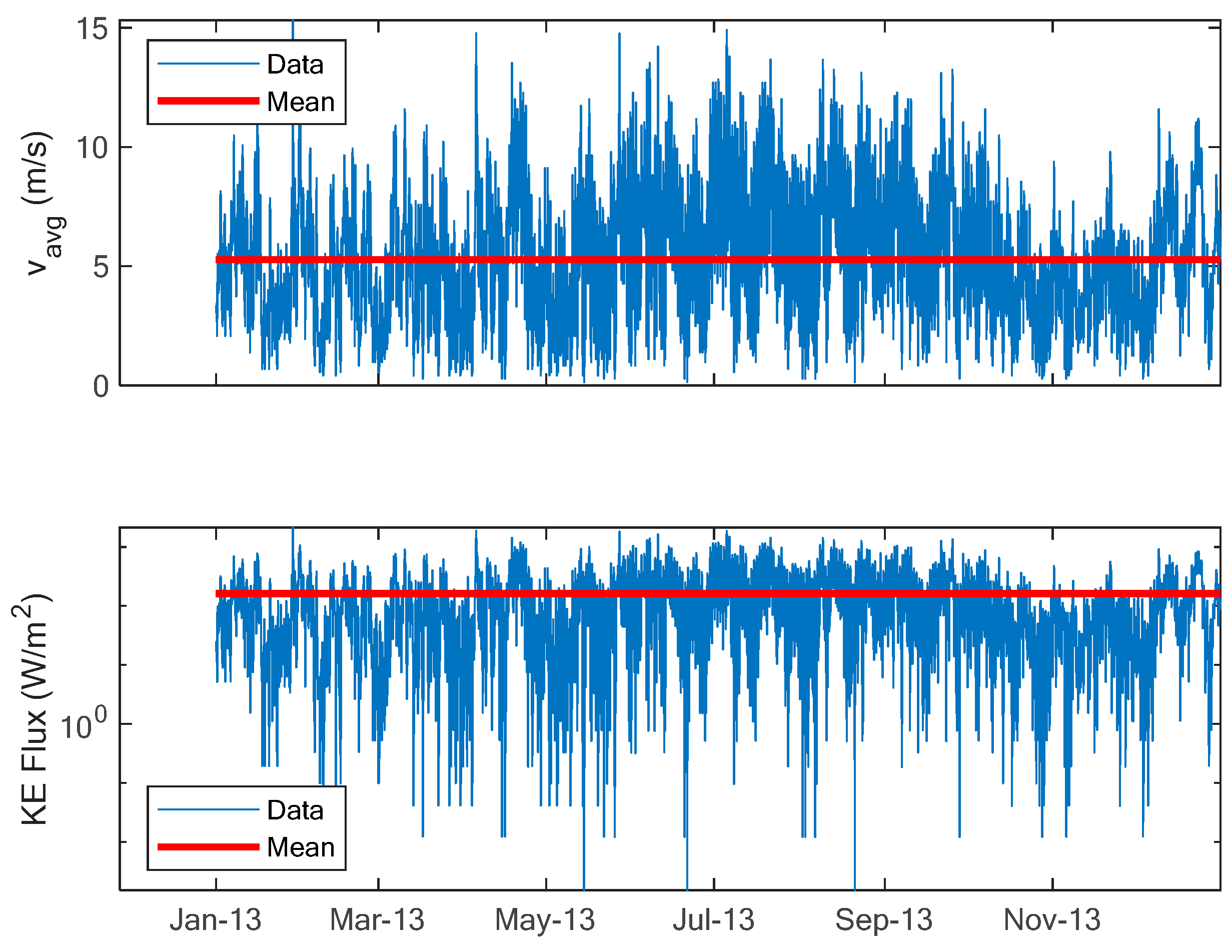
3.8. Wind Power Density
The power density, called kinetic energy flux, available from the wind for any WT to be installed at the selected site evaluated using Equation (9) is depicted in Figure 13. The estimated average power density is 163 (W/m2). Based on the classes of wind power density given in [52], it appears that the selected site is designated as class 3, which generally indicates moderate wind resources, often suitable for utility-scale wind energy development.
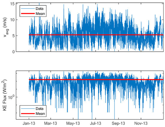
Figure 13.
The power density at Yanbu.
3.9. Annual Energy Production and Capacity Factor
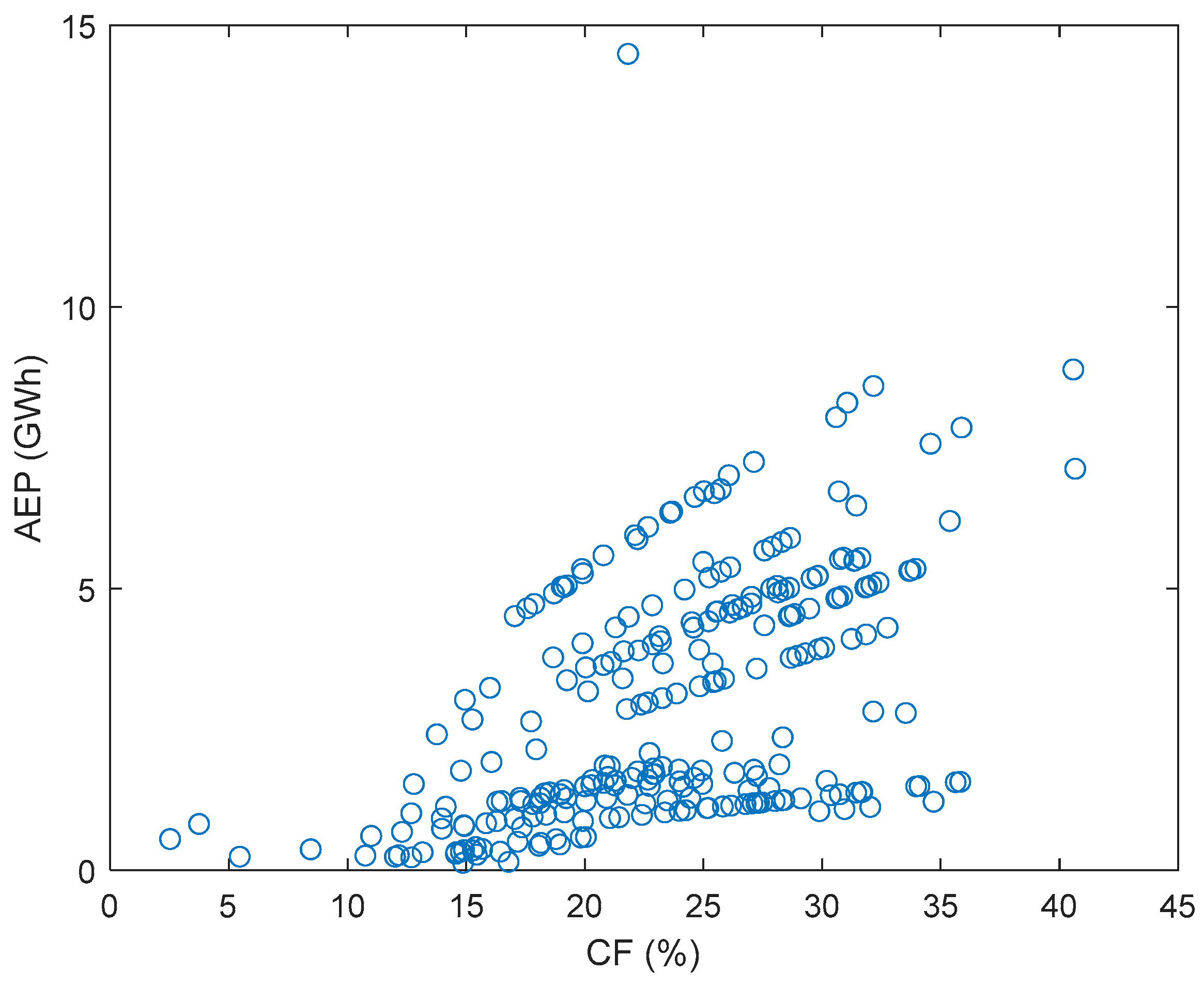
As aforementioned, the AEP and CF are very important factors for the WRA for a potential WF site. In this section both AEP and CF are evaluated for more than 100 commercial WTs, with the data found in [45]. The obtained results are represented in Figure 14 using scatter plots.
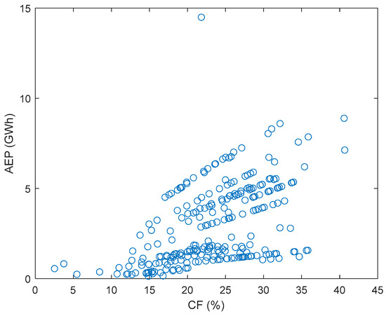
Figure 14.
AEP and CF represented as scatter plots.
The obtained results are tabulated in Table A1. The following comments, among others, can be made regarding this table:
- -
- If the WT ‘Acciona AW82/1500 kW’ is selected, it can operate at two different hub heights. At 60 m hub height, the AEP and CF are 3.35 GWh and 25.52%, whilst at 80 m, the AEP and CF are 3.80 GWh and 28.95%, respectively.
- -
- Another example is the ‘ATB Riva Calzoni ATB500’ WT. This WT can be designed to operate at two different hub heights. At 50 m hub height, the AEP and CF are 1.20 GWh and 27.48%, respectively, whilst at 70 m, the AEP and CF are 1.39 GWh and 31.66%, respectively.
- -
- The ‘Enercon E48/400 kW’ can operate with four different hub heights, which are 50 m, 55.6 m, 60 m, and 75.6 m. The AEP for these for heights is 1.05 GWh, 1.08 GWh, 1.12 GWh, and 1.22 GWh, respectively. The CF for the four available heights is 29.88%, 30.95%, 32.03%, and 34.70%, respectively.
- -
- As mentioned, it is reported in [32] that the CF ranges generally between 20% and 40%, where obtaining a CF greater than 30% is the target. However, some solutions do not satisfy this constraint. For example, the ‘Acciona AW85/1500 kW’ with a 60 m hub height has an AEP and a CF of 35.53 GWh and 25.52%, respectively. Another example is the ‘Acciona AW85/1500 kW’. This WT can have two different hub heights. For the 60 m hub height, the AEP and CF are 60 GWh and 30%, respectively, whilst for the 80 m hub height, the AEP and CF are 60 GWh and 30%, respectively.
- -
- The maximum AEP is obtained for the ‘Enercon E126/7.5 MW’, with a value of 14.49 GWh, which corresponds to a CF of 21.82%.
- -
- The minimum AEP is obtained for the ‘Northern Power d’, with a value of 0.13 GWh, which corresponds to a CF of 14.89%.
- -
- The maximum CF is obtained for the ‘Leitwind LTW104/2.0 MW’, with a value of 40.67%, which corresponds to an AEP of 7.12 GWh.
- -
- The minimum CF is obtained for the ‘Powerwind PW100/2.5 MW’, with a value of 2.52%, which corresponds to an AEP of 0.55 GWh.
- -
- Among the tested wind turbines, the ‘Enercon E101/3 MW’ and the ‘Enercon E115/2.5 MW’ can be designed to operate at the highest hub height of 149 m. For the first WT, the obtained AEP is 8.59 GWh and the obtained CF is 32.17%, and for the second WT, the obtained AEP is 8.89 GWh and the obtained CF is 40.58%.
- -
- On the other side, among the tested WTs, the ‘WindFlow W33-500’, ‘Norwin 47-STALL-225 kW’, ‘Wind Technik Nord WTN250’, ’Norwin 47-STALL-200 kW’, ‘SRC Green Power SRC31-250’, ‘Northern Power d’, and ‘AnBonus AN33/300 kW’ WTs can be designed to operate at the lowest hub height, which is 30 m. For these turbines, the AEP ranges from 0.13 GWh to 0.41 GWh and the CF ranges from 5.46% to 15.40%.
3.10. Classification of WTs Based on AEP and CF Using K-Means Clustering
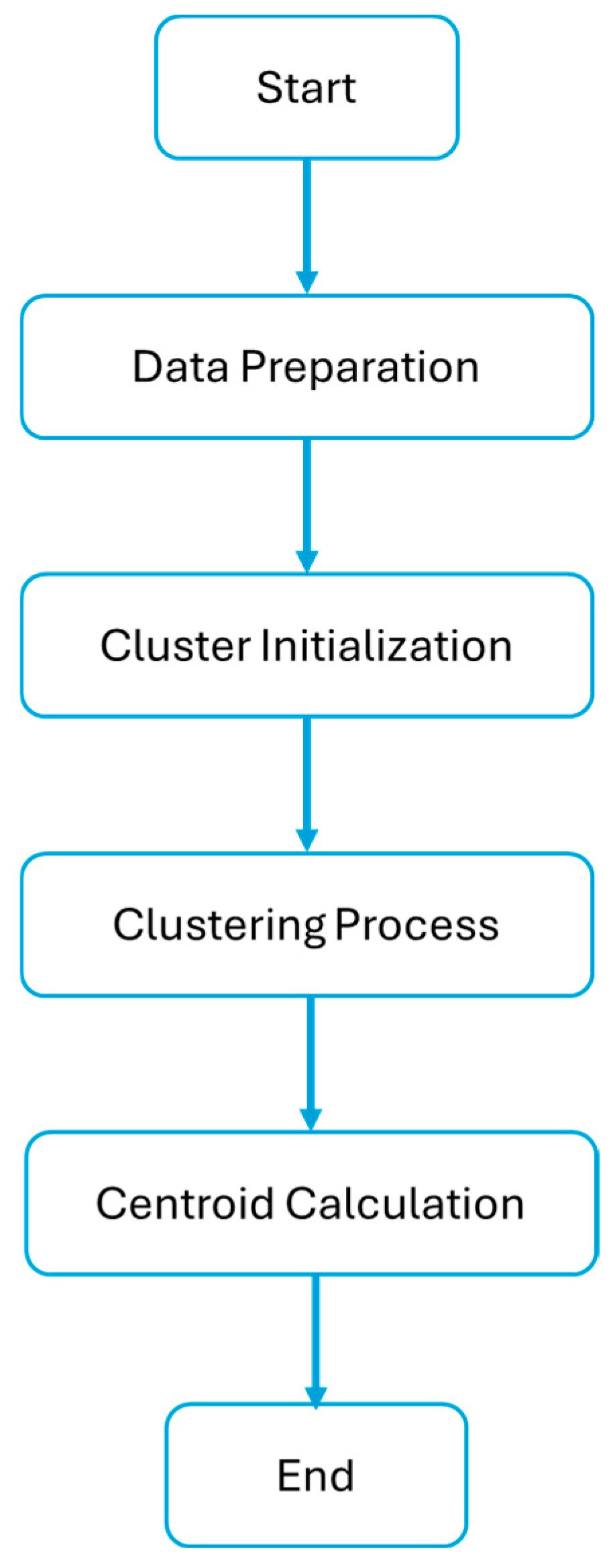
In this section, WTs are classified into different performance categories based on their AEP and CF. To achieve this classification, the K-means clustering methodology was employed to group the WTs into three distinct clusters. This unsupervised machine learning method groups WTs that share similar performance characteristics, making it an ideal approach for identifying natural groupings for WTs.
The K-means clustering methodology used here is illustrated in the flowchart shown in Figure 15, where each turbine’s AEP and CF values serve as input features for the clustering process. In this process, first the data are prepared. The AEP and CF obtained in the previous section are preprocessed for clustering. Then, the number of clusters (k = 3) is determined based on prior knowledge to classify WTs into three categories: low-, moderate-, and high-performance WTs. It is obvious that any other value of k could have been used here. After that, the K-means algorithm iteratively assigns each WT to one of the three clusters based on its proximity (Euclidean distance) to the centroids of the clusters. Finally, after each iteration, the centroids of the clusters are updated based on the average AEP and CF values of the turbines in each cluster.
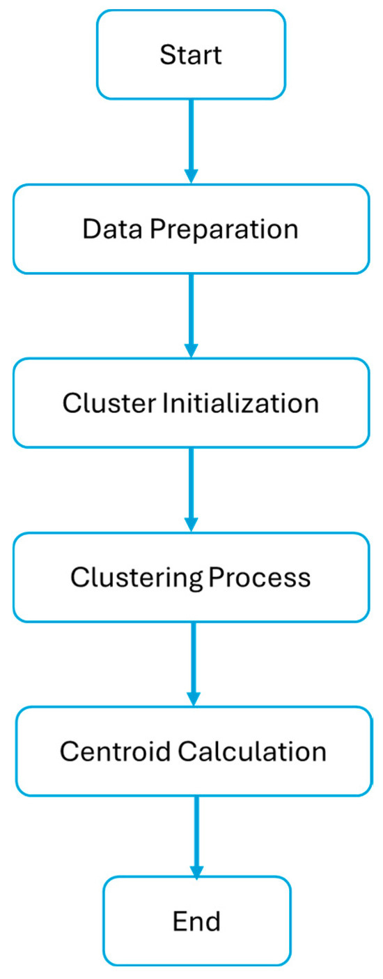
Figure 15.
K-means clustering methodology applied in this section.
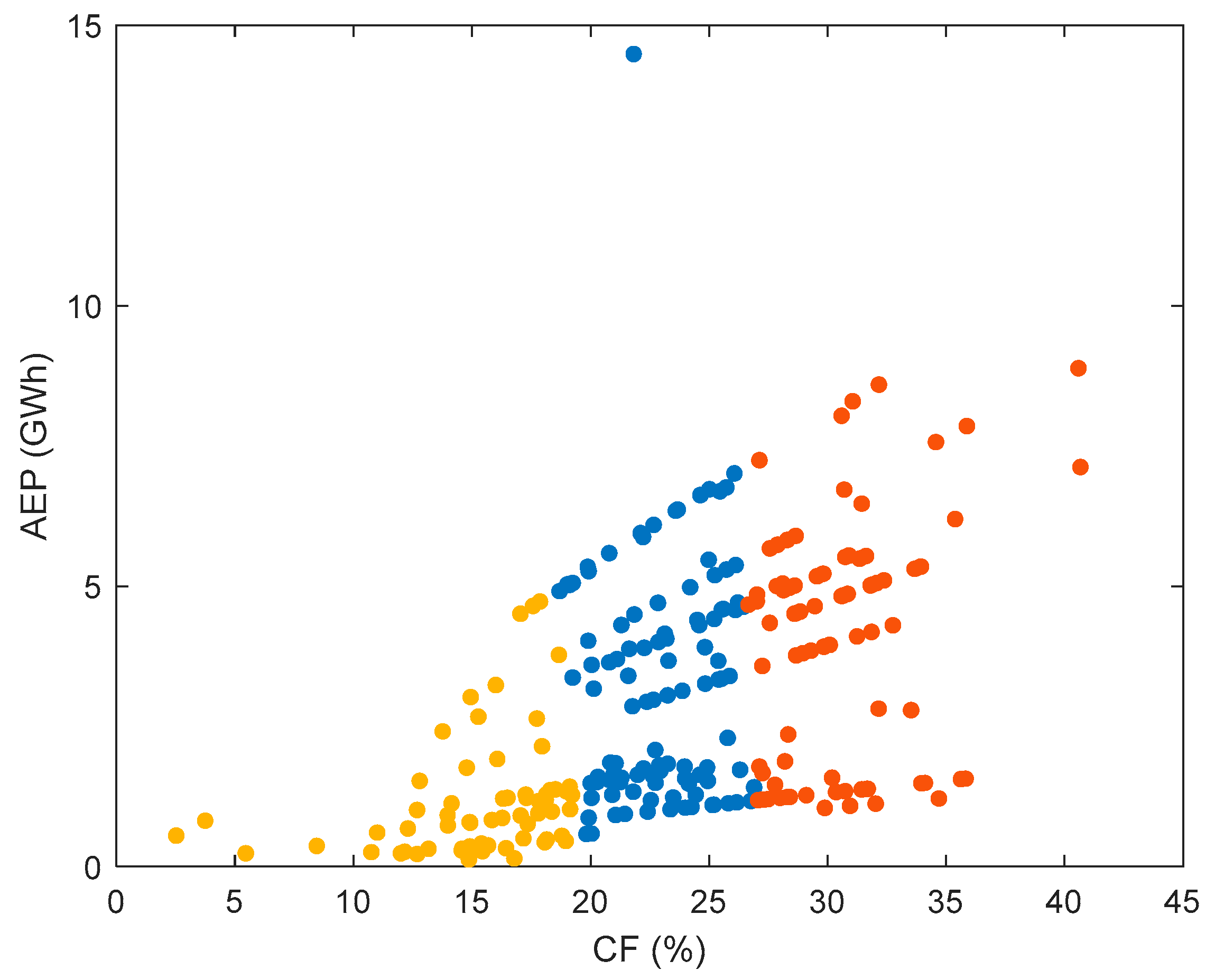
The obtained results and clusters are plotted in Figure 16, where a scatter plot is generated; each point represents a WT, and its AEP and CF values determine its position on the plot. The three different colors used on the plot provide an intuitive understanding of the distribution of WT for different clusters.
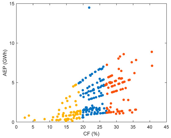
Figure 16.
K-means clustering of WTs.
As previously specified, after performing K-means clustering methodology with k = 3, the WTs were grouped into three clusters, which were classified as follows:
- -
- Cluster 1: High-Performance Turbines: These turbines exhibit high AEP and CF. WTs in this cluster are expected to have high annual energy output and efficient energy conversion.
- -
- Cluster 2: Moderate-Performance Turbines: WTs in this cluster show moderate AEP and CF. These WTs can provide a reasonable energy output but are less efficient than those in Cluster 1.
- -
- Cluster 3: Low-Performance Turbines: This group contains WTs with low AEP and CF values. WTs in this cluster are expected to have CF values below 20%. These turbines are less efficient and may not be suitable for large-scale wind energy production unless supplemented by other energy sources.
3.11. Synthetic Wind Turbine Data Generation
As mentioned, in this paper, 100 commercial WTs are investigated. Based on the previous section and the three clusters obtained, we propose here an original idea of generating new or synthetic WT data. Building upon the wind turbine classification using K-means clustering, synthetic WT data can be generated to simulate possible turbines that could be installed in a WF at a specific site. These synthetic turbines are characterized by their AEP and CF, like the turbines classified in the previous section. This approach enables the exploration of a range of new possible WT configurations that could be requested from manufacturers or installers for the selected site in Yanbu, Saudi Arabia.
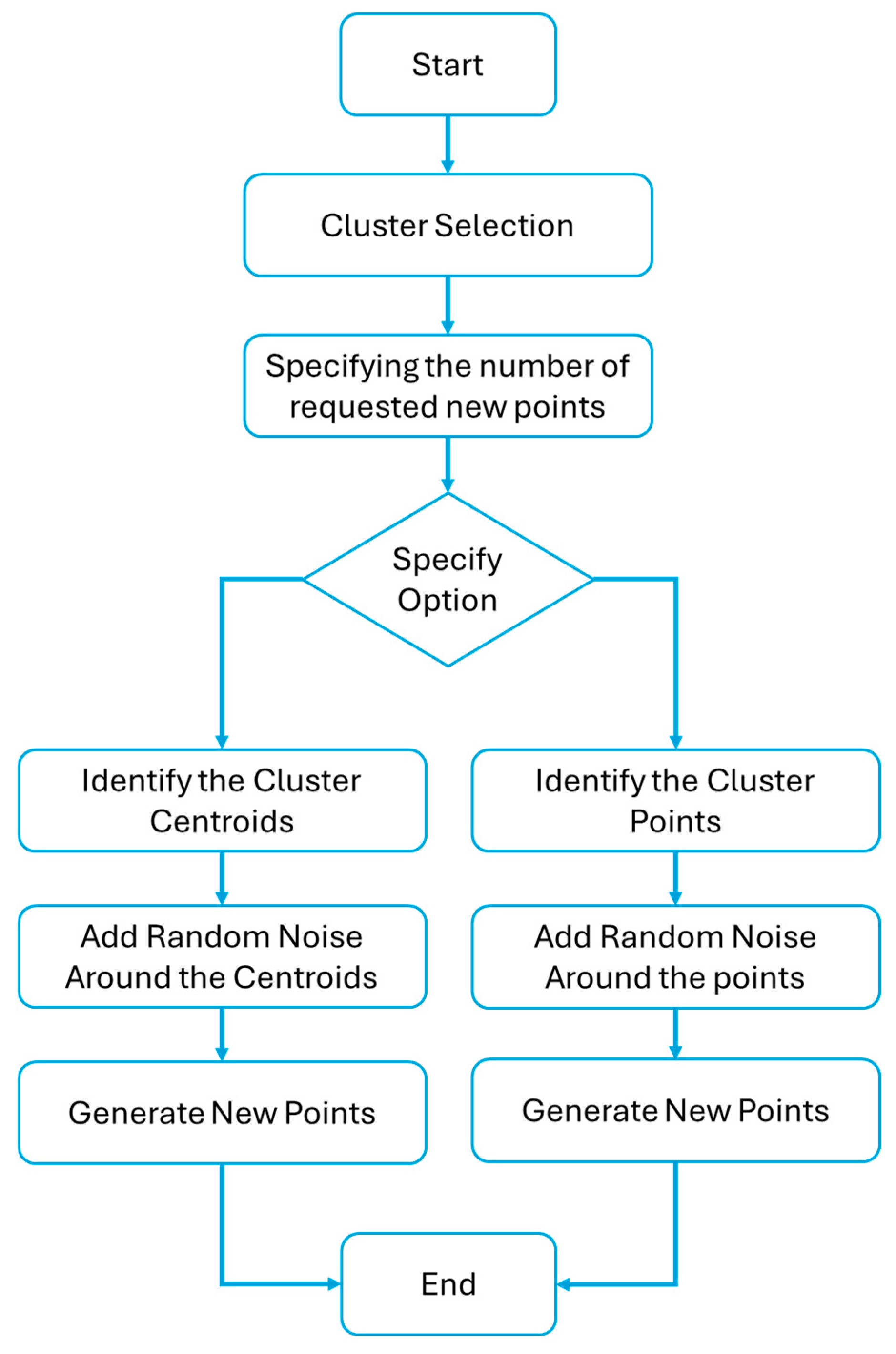
The flowchart of the proposed approach is shown in Figure 17. It starts by selecting the cluster to be used as a reference. Second, based on the number of requested new points and the option selected, there are two methods that can be used:
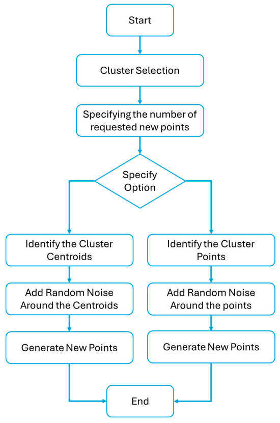
Figure 17.
The synthetic WT generation used in this section.
- -
- For the first option, the centroid obtained from the K-means clustering methodology used in the previous section represents the average AEP and CF for the selected cluster or class (high-, moderate-, or low-performance WTs). After that, to simulate real-world variability, random noise is added to the AEP and CF values of the centroid.
- -
- For the second option, noise is added directly to a number of class points obtained from the K-means clustering methodology.
Noise can be generated using a random distribution (e.g., Gaussian or uniform), which reflects the expected variability in turbine performance. In our case, we opted for a uniform random distribution.
Finally, using the noisy centroids, new synthetic data points (i.e., WTs) are created. These points will have AEP and CF values that lie within a reasonable range around the centroid values, reflecting the diversity of turbines that could be requested from manufacturers for a specific site. This process can be repeated multiple times to provide a range of possible turbines.
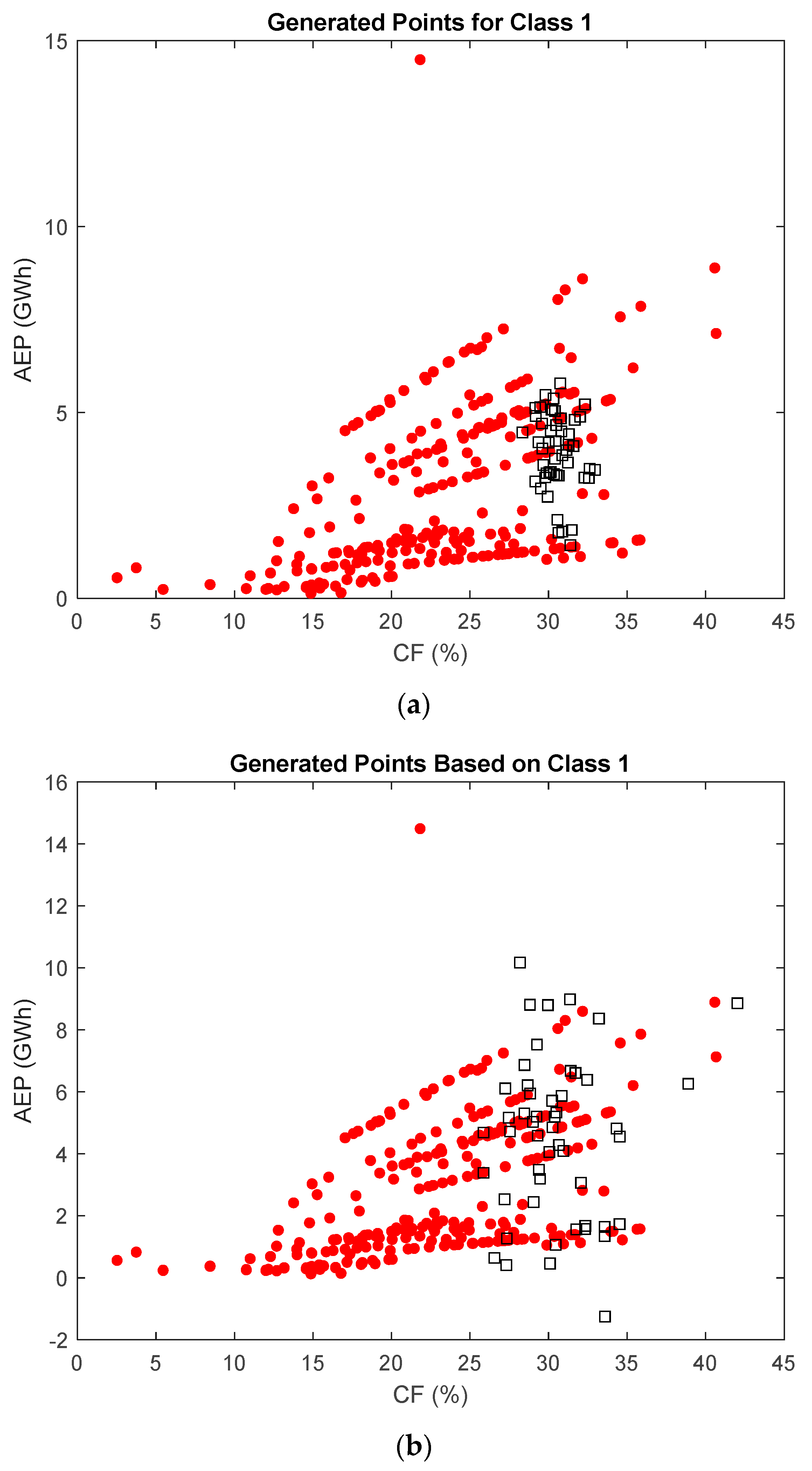
The proposed approach was applied to Cluster 1 using two different options, as explained earlier. The results are presented in Figure 18, where (a) corresponds to the first approach and (b) to the second approach. It is worth noting that in Figure 18, red dots represent real data, while square dots indicate the newly generated synthetic data points.
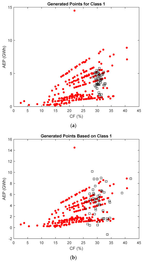
Figure 18.
Synthetic WT generation (a) using centroids and (b) using cluster points, where red dots represent real data while square dots indicate the newly generated synthetic data points.
It is worth mentioning here that K-means clustering was chosen for this study due to its efficiency, scalability, and ability to identify natural groupings within WT performance data. Given the large dataset of over 100 commercial wind turbines, K-means provides a computationally efficient method for classifying turbines based on key performance metrics, such as CF and AEP. The centroids derived from K-means offer interpretable insights, allowing wind farm developers to categorize turbines and select the most suitable models for the site, as explained in our paper. Additionally, K-means facilitates the generation of synthetic turbine datasets by introducing controlled variations around cluster centroids, enabling the development of potential new WT configurations. Compared to alternative methods like hierarchical clustering, which is computationally intensive, or Gaussian mixture models, which assume an underlying probability distribution, K-means provides a balance between accuracy and efficiency, making it an optimal choice for this study.
4. Conclusions
In this paper, a comprehensive WRA approach was proposed and applied to a potential site in the city of Yanbu in the Kingdom of Saudi Arabia. The data (wind speed, wind direction, and temperature) for one year were used. These data were scanned to preserve only data that can pass the quality assurance test. Wind speed and wind direction were analyzed to detect patterns and trends and to select the position of the WT to be placed in the WF. Furthermore, more than 100 commercial WTs were used in this study to determine the AEP and the CF of the selected site. It was demonstrated that increasing hub height improves AEP and CF, as seen with the Acciona AW82/1500 kW (AEP of 3.35 GWh to 3.80 GWh, CF of 25.52% to 28.95%) and the ATB Riva Calzoni ATB500 (AEP of 1.20 GWh to 1.39 GWh, CF of 27.48% to 31.66%). The Enercon E126/7.5 MW achieves the highest AEP (14.49 GWh), while the Leitwind LTW104/2.0 MW has the highest CF (40.67%). In contrast, the Powerwind PW100/2.5 MW records the lowest CF (2.52%). The Enercon E101/3 MW and E115/2.5 MW, operating at 149 m, achieve CFs of 32.17% and 40.58%, respectively. Conversely, turbines at 30 m hub height have AEPs between 0.13 GWh and 0.41 GWh, with CFs ranging from 5.46% to 15.40%.
In addition, the classification of WTs into three different classes was performed using K-means clustering methodology. Based on this classification, the synthetic data of potential new WTs were determined. These synthetic data allow WF developers to request turbines with specified characteristics from manufacturers, based on the site’s wind resources and the desired turbine performance class.
The obtained results are very interesting, and they offer many options to the site designer. Moreover, the results of this study are useful for accelerating the development of wind energy, not only for Saudi Arabia but also for other countries around the globe.
Finally, the findings of this study open several promising directions for future research, which can be summarized as follows:
- −
- Explore and compare ML techniques for imputing missing or failed data;
- −
- Assess the impact of AI-based data recovery on the accuracy of WRA;
- −
- Validate the synthetic WT data using physics-based simulation models and manufacturer specifications;
- −
- Compare the performance of synthetic WTs against real-world operational data to ensure robustness and practical applicability;
- −
- Utilize the generated synthetic WT data to support manufacturers in designing new turbines optimized for site-specific conditions;
- −
- Investigate alternative clustering methods (e.g., hierarchical clustering, Gaussian mixture models) to benchmark and potentially enhance the classification of WT;
- −
- Extend the analysis to include economic performance metrics such as LCOE, in addition to AEP and CF;
- −
- Conduct uncertainty analysis to improve the reliability and credibility of the study’s findings.
Author Contributions
Conceptualization, H.R.E.H.B. and M.A.M.R.; methodology, H.R.E.H.B. and M.A.M.R.; software, H.R.E.H.B.; validation, H.R.E.H.B. and M.A.M.R.; formal analysis, H.R.E.H.B. and M.A.M.R.; investigation, H.R.E.H.B. and M.A.M.R.; resources, H.R.E.H.B. and M.A.M.R.; writing—original draft preparation, H.R.E.H.B. and M.A.M.R.; writing—review and editing, H.R.E.H.B. and M.A.M.R.; visualization, H.R.E.H.B. and M.A.M.R.; supervision, M.A.M.R.; project administration, M.A.M.R.; funding acquisition, M.A.M.R. All authors have read and agreed to the published version of the manuscript.
Funding
The project was funded by the Deanship of Scientific Research (DSR) at King Abdulaziz University, Jeddah, under grant No. G: 142-135-1441. The authors, therefore, acknowledge with thanks the DSR for technical and financial support.
Institutional Review Board Statement
Not applicable.
Informed Consent Statement
Not applicable.
Data Availability Statement
The original contributions presented in this study are included in the article. Further inquiries can be directed to the corresponding author.
Conflicts of Interest
The authors declare no conflicts of interest.
Nomenclature and Abbreviations
| Symbol or Abbreviation | Description |
| Turbulence intensity | |
| Mean wind speed | |
| Average speed measured | |
| Cut-in Wind Speed (minimum wind speed at which the wind turbine starts generating power) | |
| Cut-out Wind Speed (maximum wind speed at which the turbine operates) | |
| Maximum wind speed considered | |
| Rated Wind Speed (wind speed at which the turbine generates its maximum (rated) power output) | |
| Roughness length | |
| Area of the rotor | |
| AEP | Annual energy production |
| AI | Artificial intelligence |
| ANFIS | Adaptive neuro-fuzzy inference system |
| ANN | Artificial neural network |
| CE | Cross-entropy |
| CF | Capacity factor |
| Energy produced by a given WT | |
| GEV | Generalized extreme value |
| GIS | Geographical information system |
| IEC | International electrochemical commission |
| Shape parameter | |
| LCOE | Levelized Cost of Energy |
| Power density | |
| PRF | Power reduction factor |
| Time period over which energy is calculated | |
| Wind speed | |
| Wind speed at height | |
| Wind speed at height | |
| WF | Wind farm |
| WRA | Wind resource assessment |
| WT | Wind turbine |
| Roughness exponent | |
| Yaw misalignment angle between the turbine rotor and the local wind direction | |
| Scale parameter | |
| Air density | |
| Standard deviation |
Appendix A

Table A1.
Obtained results for the estimation of AEP and CF in the function of WTs.
Table A1.
Obtained results for the estimation of AEP and CF in the function of WTs.
| WT Type | Hub Height (m) | AEP (GWh) | CF (%) |
|---|---|---|---|
| Acciona AW82/1500 kW | 60 | 3.35 | 25.52 |
| Acciona AW82/1500 kW | 80 | 3.80 | 28.95 |
| AnBonus AN33/300 kW | 30 | 0.41 | 15.40 |
| AnBonus AN33/300 kW | 40 | 0.48 | 18.15 |
| Enercon E33/330 kW | 37 | 0.50 | 17.17 |
| Enercon E33/330 kW | 44 | 0.55 | 18.79 |
| Enercon E33/330 kW | 49 | 0.58 | 19.82 |
| Enercon E33/330 kW | 50 | 0.59 | 20.05 |
| AnBonus AN41/600 kW | 42.3 | 0.61 | 11.00 |
| AnBonus AN41/600 kW | 50 | 0.68 | 12.30 |
| AnBonus AN44/600 kW | 42 | 0.80 | 14.90 |
| AnBonus AN44/600 kW | 50 | 0.87 | 16.28 |
| AnBonus AN44/600 kW | 55 | 0.91 | 17.05 |
| AnBonus AN44/600 kW | 58 | 0.95 | 17.80 |
| ATB Riva Calzoni ATB500 | 50 | 1.20 | 27.48 |
| ATB Riva Calzoni ATB500 | 70 | 1.39 | 31.66 |
| Enercon E44/900 kW | 45 | 1.01 | 12.69 |
| Enercon E44/900 kW | 55 | 1.13 | 14.14 |
| Enercon E48/400 kW | 50 | 1.05 | 29.88 |
| Enercon E48/400 kW | 55.6 | 1.08 | 30.95 |
| Enercon E48/400 kW | 60 | 1.12 | 32.03 |
| Enercon E48/400 kW | 75.6 | 1.22 | 34.70 |
| Enercon E48/500 kW | 50 | 1.10 | 25.15 |
| Enercon E48/500 kW | 55 | 1.15 | 26.17 |
| Enercon E48/500 kW | 60 | 1.19 | 27.23 |
| Enercon E48/500 kW | 76 | 1.33 | 30.36 |
| Enercon E48/600 kW | 50 | 1.18 | 22.55 |
| Enercon E48/600 kW | 55.6 | 1.23 | 23.49 |
| Enercon E48/600 kW | 60 | 1.28 | 24.44 |
| Enercon E48/600 kW | 75.6 | 1.41 | 26.90 |
| Enercon E48/700 kW | 50 | 1.23 | 20.04 |
| Enercon E48/700 kW | 55.6 | 1.28 | 20.92 |
| Enercon E48/700 kW | 60 | 1.34 | 21.80 |
| Enercon E48/700 kW | 75.6 | 1.48 | 24.15 |
| Enercon E48/800 kW | 50 | 1.23 | 17.30 |
| Enercon E48/800 kW | 55.6 | 1.29 | 18.14 |
| Enercon E48/800 kW | 60 | 1.35 | 18.98 |
| Enercon E48/800 kW | 75.6 | 1.51 | 21.25 |
| Enercon E53/500 | 60 | 1.38 | 31.43 |
| Enercon E53/500 | 73 | 1.49 | 33.96 |
| Enercon E53/600 | 60 | 1.46 | 27.78 |
| Enercon E53/600 | 73 | 1.59 | 30.19 |
| Enercon E53/700 | 60 | 1.53 | 24.95 |
| Enercon E53/700 | 73 | 1.67 | 27.25 |
| Enercon E53/750 | 60 | 1.58 | 23.99 |
| Enercon E53/750 | 73 | 1.73 | 26.31 |
| Enercon E53/800 | 60 | 1.61 | 22.65 |
| Enercon E53/800 | 73 | 1.77 | 24.92 |
| Enercon E70/2.3 MW | 57 | 3.02 | 14.94 |
| Enercon E70/2.3 MW | 64 | 3.24 | 16.00 |
| Enercon E70/2.3 MW | 85 | 3.78 | 18.66 |
| Enercon E70/2.3 MW | 98 | 4.03 | 19.90 |
| Enercon E70/2.3 MW | 113 | 4.31 | 21.30 |
| Enercon E82 E1/2 MW | 78 | 4.40 | 24.50 |
| Enercon E82 E1/2 MW | 85 | 4.60 | 25.59 |
| Enercon E82 E1/2 MW | 98 | 4.85 | 27.02 |
| Enercon E82 E1/2 MW | 108 | 5.05 | 28.11 |
| Enercon E82 E1/2 MW | 138 | 5.55 | 30.90 |
| Enercon E82 E2/2.3 MW | 78 | 4.50 | 21.85 |
| Enercon E82 E2/2.3 MW | 85 | 4.70 | 22.84 |
| Enercon E82 E2/2.3 MW | 98 | 4.98 | 24.20 |
| Enercon E82 E2/2.3 MW | 108 | 5.20 | 25.24 |
| Enercon E82 E2/2.3 MW | 138 | 5.74 | 27.89 |
| Enercon E82 E3/3 MW | 78 | 4.51 | 17.05 |
| Enercon E82 E3/3 MW | 85 | 4.73 | 17.87 |
| Enercon E82 E3/3 MW | 98 | 5.03 | 19.03 |
| Enercon E82 E3/3 MW | 108 | 5.27 | 19.92 |
| Enercon E82 E3/3 MW | 138 | 5.88 | 22.22 |
| Enercon E82 E4/3 MW | 78 | 4.51 | 17.05 |
| Enercon E82 E4/3 MW | 84 | 4.65 | 17.57 |
| Enercon E92/2.35 MW | 84 | 5.30 | 25.74 |
| Enercon E92/2.35 MW | 85 | 5.38 | 26.12 |
| Enercon E92/2.35 MW | 98 | 5.67 | 27.57 |
| Enercon E92/2.35 MW | 104 | 5.83 | 28.30 |
| Enercon E92/2.35 MW | 108 | 5.90 | 28.65 |
| Enercon E92/2.35 MW | 138 | 6.47 | 31.44 |
| Enercon E101/3 MW | 99 | 7.25 | 27.13 |
| Enercon E101/3 MW | 135 | 8.30 | 31.06 |
| Enercon E101/3 MW | 149 | 8.59 | 32.17 |
| Enercon E115/2.5 MW | 92.5 | 7.57 | 34.57 |
| Enercon E115/2.5 MW | 149 | 8.89 | 40.58 |
| Enercon E126/7.5 MW | 135 | 14.49 | 21.82 |
| RRB/Vestas V47/500 | 33.2 | 0.76 | 17.35 |
| RRB/Vestas V47/500 | 50 | 0.94 | 21.45 |
| RRB/Vestas V47/500 | 60 | 1.02 | 23.37 |
| Gamesa G52/500 kW | 44 | 1.13 | 25.82 |
| Gamesa G52/500 kW | 49 | 1.19 | 27.07 |
| Gamesa G52/500 kW | 55 | 1.24 | 28.41 |
| Gamesa G52/500 kW | 65 | 1.35 | 30.74 |
| Gamesa G58/500 kW | 44 | 1.27 | 29.10 |
| Gamesa G58/500 kW | 55 | 1.39 | 31.69 |
| Gamesa G58/500 kW | 65 | 1.49 | 34.11 |
| Gamesa G58/500 kW | 74 | 1.56 | 35.63 |
| Gamesa G52/850 kW | 44 | 1.23 | 16.49 |
| Gamesa G52/850 kW | 55 | 1.38 | 18.52 |
| Gamesa G52/850 kW | 65 | 1.51 | 20.27 |
| Gamesa G58/850 kW | 49 | 1.55 | 20.79 |
| Gamesa G58/850 kW | 55 | 1.64 | 21.99 |
| Gamesa G58/850 kW | 65 | 1.78 | 23.97 |
| lagerwey L82/2000 kW | 80 | 4.07 | 23.20 |
| lagerwey L82/2000 kW | 105 | 4.57 | 26.11 |
| Leitwind LTW77/950 kW | 65 | 2.79 | 33.52 |
| Leitwind LTW77/1.0 MW | 65 | 2.82 | 32.15 |
| Leitwind LTW70/1.7 MW | 60 | 2.64 | 17.74 |
| Leitwind LTW70/2.0 MW | 60 | 2.67 | 15.27 |
| Leitwind LTW70/2.0 MW | 60 | 2.41 | 13.77 |
| Leitwind LTW77/1.5 MW | 61.5 | 2.94 | 22.37 |
| Leitwind LTW77/1.5 MW | 65 | 3.06 | 23.25 |
| Leitwind LTW77/1.5 MW | 80 | 3.34 | 25.40 |
| Leitwind LTW77/1.5 MW | 61.5 | 2.86 | 21.76 |
| Leitwind LTW77/1.5 MW | 65 | 2.98 | 22.65 |
| Leitwind LTW77/1.5 MW | 80 | 3.26 | 24.84 |
| Leitwind LTW80/1.5 MW | 60 | 3.40 | 25.87 |
| Leitwind LTW80/1.5 MW | 80 | 3.85 | 29.30 |
| Leitwind LTW80/1.5 MW | 100 | 4.19 | 31.85 |
| Leitwind LTW80/1.8 MW | 60 | 3.40 | 21.59 |
| Leitwind LTW80/1.8 MW | 80 | 3.91 | 24.82 |
| Leitwind LTW80/1.5 MW | 60 | 3.14 | 23.87 |
| Leitwind LTW80/1.5 MW | 80 | 3.58 | 27.24 |
| Leitwind LTW80/1.5 MW | 100 | 3.92 | 29.84 |
| Leitwind LTW80/1.8 MW | 60 | 3.17 | 20.13 |
| Leitwind LTW80/1.8 MW | 80 | 3.67 | 23.29 |
| Leitwind LTW86/1.5 MW | 80 | 3.95 | 30.09 |
| Leitwind LTW86/1.5 MW | 100 | 4.30 | 32.76 |
| Leitwind LTW86/1.5 MW | 80 | 3.77 | 28.68 |
| Leitwind LTW86/1.5 MW | 100 | 4.11 | 31.24 |
| Leitwind LTW101/3.0 MW | 97 | 6.69 | 25.46 |
| Leitwind LTW101/3.0 MW | 95 | 6.76 | 25.73 |
| Leitwind LTW101/3.0 MW | 143 | 8.04 | 30.59 |
| Leitwind LTW104/2.0 MW | 95 | 6.20 | 35.38 |
| Leitwind LTW104/2.0 MW | 143 | 7.12 | 40.67 |
| Leitwind LTW104/2.5 MW | 95 | 6.72 | 30.70 |
| Leitwind LTW104/2.5 MW | 143 | 7.86 | 35.87 |
| Neg-Micon NM-48/600 | 46 | 0.98 | 18.37 |
| Neg-Micon NM-48/600 | 50 | 1.03 | 19.14 |
| Neg-Micon M750 | 36 | 0.35 | 15.28 |
| Nordex N60/1300 kW | 46 | 1.53 | 12.79 |
| Nordex N60/1300 kW | 60 | 1.77 | 14.78 |
| Nordex N60/1300 kW | 69 | 1.92 | 16.07 |
| Nordex N60/1300 kW | 85 | 2.15 | 17.95 |
| Northern Power d | 37 | 0.15 | 16.78 |
| Northern Power d | 30 | 0.13 | 14.87 |
| Norwin 47-STALL-200 kW | 30 | 0.23 | 12.69 |
| Norwin 47-STALL-200 kW | 40 | 0.27 | 15.44 |
| Norwin 47-STALL-225 kW | 30 | 0.24 | 12.00 |
| Norwin 47-STALL-225 kW | 40 | 0.29 | 14.57 |
| Norwin 47-STALL-225 kW | 50 | 0.33 | 16.44 |
| Norwin 47-ASR-500 kW | 40 | 0.87 | 19.92 |
| Norwin 47-ASR-500 kW | 65 | 1.10 | 25.20 |
| Norwin 47-ASR-750 kW | 40 | 0.92 | 13.97 |
| Norwin 47-ASR-750 kW | 65 | 1.19 | 18.11 |
| Norwin 54-ASR-750 kW | 40 | 1.17 | 17.82 |
| Norwin 54-ASR-750 kW | 65 | 1.49 | 22.74 |
| Powerwind PW56/500 kW | 44 | 1.17 | 26.77 |
| Powerwind PW56/500 kW | 46 | 1.20 | 27.33 |
| Powerwind PW56/500 kW | 49 | 1.23 | 28.00 |
| Powerwind PW56/500 kW | 50 | 1.24 | 28.31 |
| Powerwind PW56/900 kW | 59 | 1.65 | 20.98 |
| Powerwind PW56/900 kW | 71 | 1.81 | 22.90 |
| Powerwind PW56/900 kW | 59 | 1.60 | 20.31 |
| Powerwind PW56/900 kW | 71 | 1.75 | 22.23 |
| Powerwind PW60/850 kW | 70 | 1.71 | 22.94 |
| Powerwind PW90/2.5 MW | 98 | 5.47 | 24.99 |
| Powerwind PW100/2.5 MW | 80 | 0.55 | 2.52 |
| Powerwind PW100/2.5 MW | 100 | 0.82 | 3.74 |
| REPower MM82/2.0 MW | 59 | 3.37 | 19.25 |
| REPower MM82/2.0 MW | 69 | 3.64 | 20.79 |
| REPower MM82/2.0 MW | 80 | 3.90 | 22.27 |
| REPower MM82/2.0 MW | 100 | 4.31 | 24.58 |
| REPower MM82/2050 kW | 59 | 3.60 | 20.05 |
| REPower MM82/2050 kW | 69 | 3.89 | 21.64 |
| REPower MM82/2050 kW | 80 | 4.15 | 23.13 |
| REPower MM82/2050 kW | 100 | 4.59 | 25.54 |
| REPower MM92/2050 kW | 68.5 | 4.71 | 26.21 |
| REPower MM92/2050 kW | 78.5 | 5.00 | 27.86 |
| REPower MM92/2050 kW | 80 | 5.05 | 28.10 |
| REPower MM92/2050 kW | 100 | 5.52 | 30.75 |
| SRC Green Power SRC31-250 | 30 | 0.33 | 14.78 |
| Suslon S64/950 kW | 80 | 2.36 | 28.34 |
| Turbowinds T500/48 | 50 | 0.98 | 22.41 |
| Turbowinds T500/48 | 60 | 1.06 | 24.26 |
| Unison U50/750 kW | 50 | 1.28 | 19.22 |
| Unison U54/750 kW | 60 | 1.64 | 24.61 |
| Unison U57/750 kW | 68 | 1.88 | 28.20 |
| Unison U88/2000 kW | 80 | 3.70 | 21.11 |
| Unison U93/2000 kW | 80 | 4.01 | 22.86 |
| Vergnet GEV MP R 32/275 kW | 32 | 0.32 | 13.16 |
| Vergnet GEV MP R 30/275 kW | 32 | 0.26 | 10.75 |
| Vergnet GEV MP C 32/275 kW | 55 | 0.44 | 18.07 |
| Vergnet GEV MP C 32/275 kW | 60 | 0.46 | 18.95 |
| Vergnet GEV MP C 30/275 kW | 55 | 0.36 | 14.91 |
| Vergnet GEV MP C 30/275 kW | 60 | 0.38 | 15.67 |
| Vergnet GEV HP 62/1000 kW | 70 | 1.84 | 21.06 |
| Vestas V44/600 kW | 40 | 0.73 | 13.98 |
| Vestas V44/600 kW | 45 | 0.78 | 14.92 |
| Vestas V44/600 kW | 50 | 0.83 | 15.84 |
| Vestas V52/104.2 dBA | 44 | 1.21 | 16.31 |
| Vestas V52/104.2 dBA | 49 | 1.29 | 17.27 |
| Vestas V52/104.2 dBA | 55 | 1.36 | 18.30 |
| Vestas V52/104.2 dBA | 60 | 1.42 | 19.12 |
| Vestas V52/104.2 dBA | 65 | 1.49 | 20.01 |
| Vestas V52/104.2 dBA | 74 | 1.59 | 21.30 |
| Vestas V52/104.2 dBA | 86 | 1.70 | 22.87 |
| Vestas V90/1800 kW (0) | 80 | 4.55 | 28.84 |
| Vestas V90/1800 kW (0) | 95 | 4.86 | 30.85 |
| Vestas V90/1800 kW (0) | 105 | 5.06 | 32.07 |
| Vestas V90/1800 kW (0) | 125 | 5.35 | 33.94 |
| Vestas V90/1800 kW (1) | 80 | 4.52 | 28.67 |
| Vestas V90/1800 kW (1) | 95 | 4.84 | 30.67 |
| Vestas V90/1800 kW (1) | 105 | 5.03 | 31.89 |
| Vestas V90/1800 kW (1) | 125 | 5.32 | 33.73 |
| Vestas V90/1800 kW (2) | 80 | 4.35 | 27.56 |
| Vestas V90/1800 kW (2) | 95 | 4.65 | 29.46 |
| Vestas V90/1800 kW (2) | 105 | 4.83 | 30.63 |
| Vestas V90/1800 kW (2) | 125 | 5.11 | 32.38 |
| Vestas V90/1800 kW (3) | 80 | 4.51 | 28.60 |
| Vestas V90/1800 kW (3) | 95 | 4.82 | 30.59 |
| Vestas V90/1800 kW (3) | 105 | 5.02 | 31.81 |
| Vestas V90/1800 kW (3) | 125 | 5.31 | 33.67 |
| Vestas V90/2000 kW (0) | 80 | 4.67 | 26.66 |
| Vestas V90/2000 kW (0) | 95 | 5.01 | 28.61 |
| Vestas V90/2000 kW (0) | 105 | 5.22 | 29.80 |
| Vestas V90/2000 kW (0) | 125 | 5.54 | 31.62 |
| Vestas V90/2000 kW (1) | 80 | 4.63 | 26.43 |
| Vestas V90/2000 kW (1) | 95 | 4.97 | 28.37 |
| Vestas V90/2000 kW (1) | 105 | 5.18 | 29.55 |
| Vestas V90/2000 kW (1) | 125 | 5.49 | 31.35 |
| Vestas V90/2000 kW (2) | 80 | 4.42 | 25.21 |
| Vestas V90/2000 kW (2) | 95 | 4.73 | 27.02 |
| Vestas V90/2000 kW (2) | 105 | 4.93 | 28.14 |
| Vestas V90/2000 kW (2) | 125 | 5.22 | 29.82 |
| Vestas V90/2000 kW (3) | 80 | 4.63 | 26.44 |
| Vestas V90/2000 kW (3) | 95 | 4.97 | 28.38 |
| Vestas V90/2000 kW (3) | 105 | 5.18 | 29.56 |
| Vestas V90/2000 kW (3) | 125 | 5.50 | 31.38 |
| Vestas V90/3000 kW 60 Hz (mode 0) | 80 | 5.06 | 19.25 |
| Vestas V90/3000 kW 60 Hz (mode 1) | 80 | 5.02 | 19.11 |
| Vestas V90/3000 kW 60 Hz (mode 2) | 80 | 4.91 | 18.70 |
| WindFlow W33-500 | 30 | 0.24 | 5.46 |
| WindFlow W33-500 | 50 | 0.37 | 8.45 |
| Wind Technik Nord WTN250 | 30 | 0.27 | 12.16 |
| Wind Technik Nord WTN250 | 40 | 0.32 | 14.59 |
| Wind Technik Nord WTN500 | 50 | 0.92 | 21.06 |
| Wind Technik Nord WTN500 | 65 | 1.05 | 23.99 |
| WinWinD WWD56/1000 | 80 | 1.86 | 20.83 |
| WinWinD WWD-1/60 | 70 | 2.08 | 22.73 |
| WinWinD WWD64/1000 | 80 | 2.29 | 25.78 |
| WinWinD WWD-3/90 | 80 | 5.35 | 19.88 |
| WinWinD WWD-3/90 | 88 | 5.59 | 20.79 |
| WinWinD WWD-3/90 | 100 | 5.95 | 22.11 |
| WinWinD WWD-3/100 | 80 | 6.09 | 22.66 |
| WinWinD WWD-3/100 | 88 | 6.35 | 23.60 |
| WinWinD WWD-3/100 | 100 | 6.73 | 25.02 |
| EWT DW54*900HH50 | 80 | 1.83 | 23.26 |
| EWT DW54*750HH50 | 80 | 1.78 | 27.13 |
| EWT DW54*500HH50 | 80 | 1.57 | 35.82 |
| WinWinD WWD-3/103 | 80 | 6.37 | 23.68 |
| WinWinD WWD-3/103 | 88 | 6.62 | 24.63 |
| WinWinD WWD-3/103 | 100 | 7.01 | 26.07 |
References
- Li, X.; Chen, Y.; Li, K.; Gao, S.; Cui, Y. The Optimal Wind Speed Product Selection for Wind Energy Assessment under Multi-Factor Constraints. Clean. Eng. Technol. 2025, 24, 100883. [Google Scholar] [CrossRef]
- REN21. Renewables 2022 Global Status; REN21: Paris, France, 2022; ISBN 9783948393045. [Google Scholar]
- Lazard. Lazard’s Levelized Cost of Energy V15.0; Lazard: Melbourne, VIC, Australia, 2021. [Google Scholar]
- Liu, J.; Xiong, G.; Suganthan, P.N. Differential Evolution-Based Mixture Distribution Models for Wind Energy Potential Assessment: A Comparative Study for Coastal Regions of China. Energy 2025, 321, 135151. [Google Scholar] [CrossRef]
- Faraz, M.I. Strategic Analysis of Wind Energy Potential and Optimal Turbine Selection in Al-Jouf, Saudi Arabia. Heliyon 2024, 10, e39188. [Google Scholar] [CrossRef]
- Li, X.; Huang, G.; Yu, W.; Yin, R.; Zheng, H. Distribution Inference of Wind Speed at Adjacent Spaces Using Generative Conditional Distribution Sampler. Comput. Electr. Eng. 2025, 123, 110123. [Google Scholar] [CrossRef]
- Dong, S.; Gong, Y.; Wang, Z.; Incecik, A. Wind and Wave Energy Resources Assessment around the Yangtze River Delta. Ocean Eng. 2019, 182, 75–89. [Google Scholar] [CrossRef]
- Zhang, H.; Cao, Y.; Zhang, Y.; Terzija, V. Quantitative Synergy Assessment of Regional Wind-Solar Energy Resources Based on MERRA Reanalysis Data. Appl. Energy 2018, 216, 172–182. [Google Scholar] [CrossRef]
- Wang, Z.; Duan, C.; Dong, S. Long-Term Wind and Wave Energy Resource Assessment in the South China Sea Based on 30-Year Hindcast Data. Ocean Eng. 2018, 163, 58–75. [Google Scholar] [CrossRef]
- Sobchenko, A.; Khomenko, I. Assessment of Regional Wind Energy Resources over the Ukraine. Energy Procedia 2015, 76, 156–163. [Google Scholar] [CrossRef]
- Chandel, S.S.; Murthy, K.S.R.; Ramasamy, P. Wind Resource Assessment for Decentralised Power Generation: Case Study of a Complex Hilly Terrain in Western Himalayan Region. Sustain. Energy Technol. Assess. 2014, 8, 18–33. [Google Scholar] [CrossRef]
- Dayal, K.K.; Cater, J.E.; Kingan, M.J.; Bellon, G.D.; Sharma, R.N. Wind Resource Assessment and Energy Potential of Selected Locations in Fiji. Renew. Energy 2021, 172, 219–237. [Google Scholar] [CrossRef]
- Saeed, M.A.; Ahmed, Z.; Hussain, S.; Zhang, W. Wind Resource Assessment and Economic Analysis for Wind Energy Development in Pakistan. Sustain. Energy Technol. Assess. 2021, 44, 101068. [Google Scholar] [CrossRef]
- Boudia, S.M.; Santos, J.A. Assessment of Large-Scale Wind Resource Features in Algeria. Energy 2019, 189, 116299. [Google Scholar] [CrossRef]
- Wan, J.; Zheng, F.; Luan, H.; Tian, Y.; Li, L.; Ma, Z.; Xu, Z.; Li, Y. Assessment of Wind Energy Resources in the Urat Area Using Optimized Weibull Distribution. Sustain. Energy Technol. Assess. 2021, 47, 101351. [Google Scholar] [CrossRef]
- Jain, A.; Das, P.; Yamujala, S.; Bhakar, R.; Mathur, J. Resource Potential and Variability Assessment of Solar and Wind Energy in India. Energy 2020, 211, 118993. [Google Scholar] [CrossRef]
- Aukitino, T.; Khan, M.G.M.; Ahmed, M.R. Wind Energy Resource Assessment for Kiribati with a Comparison of Different Methods of Determining Weibull Parameters. Energy Convers. Manag. 2017, 151, 641–660. [Google Scholar] [CrossRef]
- Kazet, M.Y.; Mouangue, R.; Kuitche, A.; Ndjaka, J.M. Wind Energy Resource Assessment in Ngaoundere Locality. Energy Procedia 2016, 93, 74–81. [Google Scholar] [CrossRef]
- Sharma, K.; Ahmed, M.R. Wind Energy Resource Assessment for the Fiji Islands: Kadavu Island and Suva Peninsula. Renew. Energy 2016, 89, 168–180. [Google Scholar] [CrossRef]
- Ramadan, H.S. Wind Energy Farm Sizing and Resource Assessment for Optimal Energy Yield in Sinai Peninsula, Egypt. J. Clean. Prod. 2017, 161, 1283–1293. [Google Scholar] [CrossRef]
- Charabi, Y.; Al-Yahyai, S.; Gastli, A. Evaluation of NWP Performance for Wind Energy Resource Assessment in Oman. Renew. Sustain. Energy Rev. 2011, 15, 1545–1555. [Google Scholar] [CrossRef]
- Ayik, A.; Ijumba, N.; Kabiri, C.; Goffin, P. Preliminary Wind Resource Assessment in South Sudan Using Reanalysis Data and Statistical Methods. Renew. Sustain. Energy Rev. 2021, 138, 110621. [Google Scholar] [CrossRef]
- Samal, R.K. Assessment of Wind Energy Potential Using Reanalysis Data: A Comparison with Mast Measurements. J. Clean. Prod. 2021, 313, 127933. [Google Scholar] [CrossRef]
- Olaofe, Z.O. Review of Energy Systems Deployment and Development of Offshore Wind Energy Resource Map at the Coastal Regions of Africa. Energy 2018, 161, 1096–1114. [Google Scholar] [CrossRef]
- Neupane, D.; Kafle, S.; Karki, K.R.; Kim, D.H.; Pradhan, P. Solar and Wind Energy Potential Assessment at Provincial Level in Nepal: Geospatial and Economic Analysis. Renew. Energy 2022, 181, 278–291. [Google Scholar] [CrossRef]
- Wang, L.; Liu, J.; Qian, F. Wind Speed Frequency Distribution Modeling and Wind Energy Resource Assessment Based on Polynomial Regression Model. Int. J. Electr. Power Energy Syst. 2021, 130, 106964. [Google Scholar] [CrossRef]
- Adedeji, P.A.; Akinlabi, S.A.; Madushele, N.; Olatunji, O.O. Neuro-Fuzzy Resource Forecast in Site Suitability Assessment for Wind and Solar Energy: A Mini Review. J. Clean. Prod. 2020, 269, 122104. [Google Scholar] [CrossRef]
- Hernández Galvez, G.; Saldaña Flores, R.; Miranda Miranda, U.; Sarracino Martínez, O.; Castillo Téllez, M.; Almenares López, D.; Gómez, A.K.T. Wind Resource Assessment and Sensitivity Analysis of the Levelised Cost of Energy. A Case Study in Tabasco, Mexico. Renew. Energy Focus 2019, 29, 94–106. [Google Scholar] [CrossRef]
- Silvera, O.C.; Chamorro, M.V.; Ochoa, G.V. Wind and Solar Resource Assessment and Prediction Using Artificial Neural Network and Semi-Empirical Model: Case Study of the Colombian Caribbean Region. Heliyon 2021, 7, e07959. [Google Scholar] [CrossRef]
- Elshafei, B.; Peña, A.; Xu, D.; Ren, J.; Badger, J.; Pimenta, F.M.; Giddings, D.; Mao, X. A Hybrid Solution for Offshore Wind Resource Assessment from Limited Onshore Measurements. Appl. Energy 2021, 298, 117245. [Google Scholar] [CrossRef]
- Teumzghi, T. Wind Resource Assessment for Possible Wind Farm Development in Dekemhare and Assab, Eritrea. Master’s Thesis, Halmstad University, Halmstad, Sweden, 2018; pp. 1–6. [Google Scholar]
- Lam, V. Development of Wind Resource Assessment Methods and Application to the Waterloo Region. Master’s Thesis, University of Waterloo, Waterloo, ON, Canada, 2013. [Google Scholar]
- Gottschall, J.; Dörenkämper, M. Understanding and Mitigating the Impact of Data Gaps on Offshore Wind Resource Estimates. Wind Energy Sci. 2021, 6, 505–520. [Google Scholar] [CrossRef]
- Coville, A.; Siddiqui, A.; Vogstad, K.O. The Effect of Missing Data on Wind Resource Estimation. Energy 2011, 36, 4505–4517. [Google Scholar] [CrossRef]
- Zapata-Sierra, A.J.; Cama-Pinto, A.; Montoya, F.G.; Alcayde, A.; Manzano-Agugliaro, F. Wind Missing Data Arrangement Using Wavelet Based Techniques for Getting Maximum Likelihood. Energy Convers. Manag. 2019, 185, 552–561. [Google Scholar] [CrossRef]
- Burton, T.; Jenkins, N.; Sharpe, D.; Bossanyi, E. Wind Energy Handbook; John Wiley & Sons, Ltd.: Chichester, UK, 2011; ISBN 9781119992714. [Google Scholar]
- Petersen, E.L.; Mortensen, N.G.; Landberg, L.; Hùjstrup, J.; Frank, H.P. Wind Power Meteorology. Part I: Climate and Turbulence. Wind Energy 1998, 1, 25–45. [Google Scholar] [CrossRef]
- Machidon, D.; Istrate, M.; Beniuga, R. Wind Shear Coefficient Estimation Based on LIDAR Measurements to Improve Power Law Extrapolation Performance. Remote Sens. 2025, 17, 23. [Google Scholar] [CrossRef]
- Meng, W.; Yang, Z.; Rao, Z.; Li, S.; Lin, X.; Peng, J.; Cao, Y.; Chen, Y. Refined Assessment Method of Offshore Wind Resources Based on Interpolation Method. Energies 2025, 18, 213. [Google Scholar] [CrossRef]
- Ray, M.L.; Rogers, A.L.; Mcgowan, J.G. Analysis of Wind Shear Models and Trends in Different Terrains. Wind. Eng. 2006, 30, 341–350. [Google Scholar]
- White, F.M. Fluid Mechanics; McGraw Hill: New York, NY, USA, 2002; ISBN 007124493X. [Google Scholar]
- IEC 61400-1; Wind Turbines—Part 1: Design Requirements, 3rd ed. International Electrotechnical Commission: Geneva, Switzerland, 2019.
- Wind Power Generation|CRC Research. Available online: https://www.crcresearch.org/node/304 (accessed on 8 July 2021).
- Ismaiel, A.M.M.; Yoshida, S. Study of Turbulence Intensity Effect on the Fatigue Lifetime of Wind Turbines. Evergr. Jt. J. Nov. Carbon Resour. Sci. Green Asia Strategy 2018, 5, 25–32. [Google Scholar] [CrossRef]
- Wind Resource Analysis and Power Curves—Edward Bodmer—Project and Corporate Finance. Available online: https://edbodmer.com/wind-financial-modelling-and-resource-analysis/ (accessed on 10 July 2021).
- Dallas, S.; Stock, A.; Hart, E. Control-Oriented Modelling of Wind Direction Variability. Wind Energy Sci. 2024, 9, 841–867. [Google Scholar] [CrossRef]
- Liew, J.; Urbán, A.M.; Andersen, S.J. Analytical Model for the Power-Yaw Sensitivity of Wind Turbines Operating in Full Wake. Wind Energy Sci. 2020, 5, 427–437. [Google Scholar] [CrossRef]
- Rediske, G.; Burin, H.P.; Rigo, P.D.; Rosa, C.B.; Michels, L.; Siluk, J.C.M. Wind Power Plant Site Selection: A Systematic Review. Renew. Sustain. Energy Rev. 2021, 148, 111293. [Google Scholar] [CrossRef]
- Rehman, S. Wind Energy Resources Assessment for Yanbo, Saudi Arabia. Energy Convers. Manag. 2004, 45, 2019–2032. [Google Scholar] [CrossRef]
- Solar Resource Maps and GIS Data for 200+ Countries|Solargis. Available online: https://solargis.com/maps-and-gis-data/download/saudi-arabia (accessed on 29 August 2020).
- Rehman, S.; Halawani, T.O.; Husain, T. Weibull Parameters for Wind Speed Distribution in Saudi Arabia. Sol. Energy 1994, 53, 473–479. [Google Scholar] [CrossRef]
- National Renewable Energy Laboratory. Wind Resource Assessment Handbook; National Renewable Energy Laboratory: Golden, CO, USA, 2010. [Google Scholar]


Disclaimer/Publisher’s Note: The statements, opinions and data contained in all publications are solely those of the individual author(s) and contributor(s) and not of MDPI and/or the editor(s). MDPI and/or the editor(s) disclaim responsibility for any injury to people or property resulting from any ideas, methods, instructions or products referred to in the content. |
© 2025 by the authors. Licensee MDPI, Basel, Switzerland. This article is an open access article distributed under the terms and conditions of the Creative Commons Attribution (CC BY) license (https://creativecommons.org/licenses/by/4.0/).