Abstract
This paper presents a comprehensive methodology to forecast the daily energy demand associated with recharging private electric vehicles in urban areas. The approach is based on plausible scenarios regarding the penetration of battery-powered vehicles and the availability of charging infrastructure. Accurate space and time forecasting of charging activities and power requirements is a critical issue in supporting the transition from conventional to battery-powered vehicles for urban mobility. This technological shift represents a key milestone toward achieving the zero-emissions target set by the European Green Deal for 2050. The methodology leverages Floating Car Data (FCD) samples. The widespread use of On-Board Units (OBUs) in private vehicles for insurance purposes ensures the methodology’s applicability across diverse geographical contexts. In addition to FCD samples, the estimation of charging demand for private electric vehicles is informed by a large-scale, detailed survey conducted by ENEA in Italy in 2023. Funded by the Ministry of Environment and Energy Security as part of the National Research on the Electric System, the survey explored individual charging behaviors during daily urban trips and was designed to calibrate a discrete choice model. To date, the methodology has been applied to the Metropolitan Area of Rome, demonstrating robustness and reliability in its results on two different scenarios of analysis. Each demand/supply scenario has been evaluated in terms of the hourly distribution of peak charging power demand, at the level of individual urban zones or across broader areas. Results highlight the role of the different components of power demand (at home or at other destinations) in both scenarios. Charging at intermediate destinations exhibits a dual peak pattern—one in the early morning hours and another in the afternoon—whereas home-based charging shows a pronounced peak during evening return hours and a secondary peak in the early afternoon, corresponding to a decline in charging activity at other destinations. Power distributions, as expected, sensibly differ from one scenario to the other, conditional to different assumptions of private and public recharge availability and characteristics.
1. Introduction
This paper presents the results of a research activity carried out by ENEA and its academic partners during the 2022–2024 period, as part of the multiannual Research Program on the Electricity System, under the supervision of the Italian Ministry of the Environment and Energy Security (MASE).
The objective of the study is to estimate daily charging profiles of private electric vehicles across different zones of an urban area, using standardized data formats to ensure methodological reproducibility. The profiles are derived as an expected outcome of electric vehicle penetration rates, incorporating projected charging infrastructure scenarios.
Estimating charging profiles for typical days of the year provides essential insights for verifying charging infrastructure suitability and determining the electrical power requirements in various urban zones. Moreover, it enables the assessment of strategies to reduce peak power demand and redistribute it evenly throughout the day, through smart charging technologies and criteria, with or without the use of bidirectional Vehicle-to-Everything (V2X) systems.
Although our study primarily focuses on assessing the impact of EV private vehicles on charging and power distribution networks, the procedure—by estimating the energy stored in vehicle batteries at the start and end of each charging session—can also be applied to evaluate V2X potential. As detailed in the following sections, the model distinguishes between charging location and type of grid access (either through public or private infrastructures), thus enabling separate assessments of V2G and V2B potential.
Figure 1 illustrates the dual role of predictive charging demand models: first, estimating power demand across the territory to optimally size charging infrastructures and power networks; second, assessing the energy stored in electric vehicle batteries over time and space to support the implementation of V2X strategies.
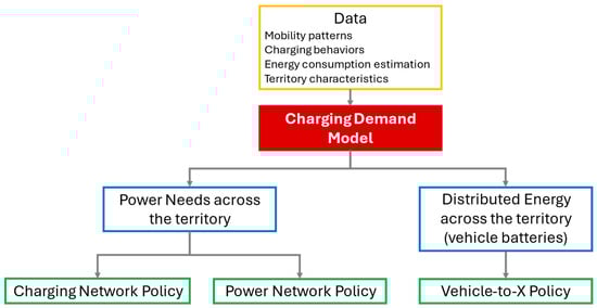
Figure 1.
Flow-chart representing the capability of predictive charging demand models for estimating: power and charging infrastructures needs across the territory, and potential of V2X, integrated both with power grids (V2G) and buildings electrical installations (V2B).
Several studies highlight the relevance of a well-designed charging infrastructure in promoting the adoption of electric mobility [1,2,3]. Design challenges are particularly complex in urban environments [4,5] where space is limited, and the demand is particularly variable and diverse.
Public charging infrastructure for individual mobility is often installed based on parking concentration criteria, statistically assuming that charging demand increases in larger parking areas or those intended for longer stays. Our research aims to refine demand analysis by estimating the probability that a vehicle will be charged during a specific stopover. This estimation considers not only the characteristics of the parking location and available charging options but also the presumed battery state of charge and the expected mobility needs following the stop. Where possible, the probability of charging is also linked to the driver’s individual profile.
To this end, an individual behavioral model was developed based on the results of a Stated Preferences (SP) survey. A previous publication [6] reviewed the state of the art in behavioral modeling for EV charging and the use of surveys for this purpose.
The model is designed to make use of FCD (Floating Car Data). FCD offers valuable, albeit partial, insights into individual mobility patterns, requiring appropriate scaling procedures to infer total mobility demand. Recent research has explored the integration of FCD with stationary sensors and opportunistic data sources to enhance representativeness and spatial coverage [7,8,9,10,11].
FCD exploitation for the estimation of private electric vehicle charging demand has been already proposed in the literature [12,13], mainly to individuate major stopover concentration across the territory and time. In other cases, individual mobility patterns are considered [14] to apply simplified behavioral paradigms. Recently, FCD potential has been investigated to not only address a smart design of recharge infrastructure but also for leveraging the potential of electric vehicles to support electricity grids [15,16]. Models for V2G applications represent a very promising research field, a source of inspiration for charge demand forecasting.
Building on the current state of the art [17], this study implements a complete FCD-based pipeline for reconstructing individual trips and travel chains, identifying approximate home and work locations, and deriving detailed mobility statistics.
Home-based travel chains derived from FCD are considered the “choice units” for applying a probabilistic behavioral charging model based on results of a large-scale Stated Preferences (SP) survey that considered many choice variables such as travel energy needs, battery state of charge (SOC), and the availability and characteristics of charging infrastructure at each stop. By simulating individual charging events, aggregate local energy demand is calculated over the day (charging profiles), enabling a probabilistic estimation of zonal charging profiles—i.e., the temporal distribution of power demand for private EV charging across different city zones.
The paper is structured as follows: Section 1 outlines the general framework of the proposed methodology; Section 2 details the key computational algorithms; and Section 3 presents results from a representative case study. The final section, Section 4, discusses the applicability of the procedure and highlights the relevance of the findings. Specific references are included in the corresponding sections.
2. Materials and Methods
2.1. Overall Procedural Scheme
The proposed procedure is based on the use of large samples of FCD, enabling the reconstruction of individual mobility patterns; these are intended as the most likely travel sequences over an analysis period sufficiently representative of a given seasonality for the entire population of residents within an urban area. A behavioral model is applied to these patterns, indicating, for each planned stop, the probability that, in the case of using a battery-powered electric vehicle (BEV), charging will be performed. This is carried out taking into account the characteristics of the stop—mainly stop duration—availability, and characteristics of charging infrastructure, the battery’s state of charge, the expected mobility needs after the stop, and the driver’s profile.
In a context where both battery power penetration and charging infrastructure are fully consolidated and known, the proposed procedure allows for the most likely demand to be assessed in different urban areas over the course of a typical day. Conversely, in contexts where the e-mobility is still evolving, both on the supply and demand sides, as is currently the case in Italy and other European countries, the analysis tool works like a classic “what-if” Decision Support System (DSS). In fact, it allows for the simulation of the effects of policies favoring a greater penetration of battery power in individual urban transport, ultimately also enabling a cost–benefit assessment of the different policy options.
Figure 2 refers to this latter type of application: FCD processing provides information on individual mobility patterns, which are then also qualified in terms of energy consumption, once the battery electric vehicle’s rate into the circulating fleet has been assumed. On the other hand, evidence on individual charging behavior provided by surveys and literature feeds a random utility model. Such a model is then applied to the mobility patterns of private vehicles assumed to be electric under different hypotheses on recharge infrastructure availability and characteristics, yielding a probabilistic estimate of charging events in different urban areas.
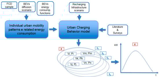
Figure 2.
Estimation of private electric cars’ urban charging profiles (CPs) from FCD. z is a generic urban zone, ti is a generic day time interval, Vi is a generic electric car, and Pi is the related probability of recharging in (z; ti).
For each time ti and urban zone z, appropriately delimited based on criteria of territorial homogeneity, the private car charging behavioral model provides a probability that each vehicle v parked in the area is charging. Given the power (kW) available to charge electric cars in that specific area, it is possible to calculate, by summation, the power absorbed for charging in the area at the generic instant t, deriving the daily zonal charging profiles.
2.2. Floating Car Exploration and Exploitation
FCD are geolocated time series generated by vehicles equipped with OBUs or integrated GPS systems capable of recording, at regular time or space intervals, position, speed, heading, engine status (on/off), and other operational attributes. FCD can be regarded as mobile sensors that opportunistically sample the road network, offering broad spatiotemporal coverage and, when properly pre-processed, valuable insights into individual travel behavior.
The FCD processing pipeline consists of a comprehensive framework designed to convert raw GPS data streams into coherent, validated, and analytically reusable mobility products. Each FCD record includes a unique trace identifier, a pseudonymized vehicle ID that remains constant throughout the observation period, a timestamp with one-second precision, geographical coordinates in WGS84 format, instantaneous speed, heading, engine status, GPS signal quality, and an odometer-based progressive distance value. Sampling frequency may vary depending on the data provider, being either time-based, such as every thirty seconds, or space-based, for example, every one or two kilometers. In the considered case study, most samples were recorded at thirty-second intervals, although more advanced on-board units can generate additional observations when abrupt changes in curvature or speed occur.
The pipeline’s main objective is to transform these heterogeneous data streams into structured and consistent analytical units suitable for quantitative transport analysis. This process begins with the verification of spatial and temporal quality through data normalization and validation, which ensures that all samples are spatially consistent and temporally ordered.
Once samples are validated, the pipeline reconstructs vehicle trajectories and generates the two main analytical entities of the system: trips and TripLegs. A trip corresponds to a continuous movement session of a vehicle, typically delimited by engine-on and engine-off conditions, or, when such information is unavailable, inferred from thresholds on speed and stop duration. Each trip is described by a sequence of ordered GPS records that include departure and arrival times, traveled distance, total duration, and average speed. From these sequences, the pipeline derives sub-segments known as TripLegs, which represent all possible pairs of chronologically sequential GPS points belonging to different traffic zones. This structure allows for a detailed assessment of travel performance, including average travel times, speeds, and distances between origin–destination pairs, and enables the construction of OD matrices and travel time skims directly from empirical data.
A robust outlier detection procedure based on the boxplot method is applied to filter anomalous TripLegs that could distort the analysis, while incomplete or noisy trajectories, such as single-sample trips or those affected by signal loss, are removed to maintain the integrity of the analytical base. The aggregation of trips and TripLegs by origin and destination zones, time periods, and day types results in the generation of observed OD matrices and performance indicators that describe spatial and temporal patterns of mobility.
Besides trajectory reconstruction, a spatial analysis module identifies stationary clusters of points, known as stay points, which represent typical stopping locations. The identification is based on the DBSCAN density-based clustering algorithm [18] applied to stationary samples within a predefined radius, with parameters tuned to the density of the urban network. For each cluster, average stop duration, variance, and recurrence are computed to characterize both short and long stops across different temporal windows. Two categories of stay points are recognized: internal stay points, located within the study area, and virtual stay points, representing points of entry or exit along the network boundaries. Virtual stay points are detected when clusters extend spatially along access corridors, and the initial odometer reading indicates prior to travel before the first recorded point. Each stay point is associated with a traffic zone and linked to trips as an origin or destination, providing spatial anchors for reconstructing travel chains.
The classification of stay points into functional types relies on duration and recurrence criteria. The stay point with the longest cumulative stop duration, accounting for at least ten percent of the total recorded time, is identified as the home location. Recurrent stops of a long duration with weekly periodicity are classified as work, while the remaining points are labeled as other. Validation of this classification using census and employment data produced determination coefficients of 0.91 for home and 0.71 for work, confirming the reliability of the method in reproducing real activity locations.
From the identified trips and classified stay points, the pipeline reconstructs home-based travel chains by chronologically ordering trips for each vehicle. Each chain starts at a trip departing from the home location and aggregates subsequent trips until the vehicle returns home. The resulting sequence of trips forms a home-based chain stored as an analytical unit. During storage, each chain is enriched with summary attributes such as total travel time, number of intermediate stops, cumulative duration, and information about preceding and following chains. The classification of these chains is based on the ordered sequence of stay point types, generating categories such as HOME–HOME, HOME–WORK–HOME, HOME–OTHER–HOME, or mixed combinations that describe different mobility behaviors. This reconstruction enables the analysis of systematic and non-systematic travel patterns at the individual level, facilitating the study of commuting behavior and the identification of daily activity structures.
Over the past two decades, generative models of human mobility have attracted increasing attention within the scientific community. The main reasons lie in their ability to overcome issues related to the use of personal or sensitive data (such as those derived from vehicle GPSs or mobile phone records), while also ensuring scalability when available datasets are incomplete or not representative. Moreover, they allow researchers to extract global behavioral patterns and universal laws that can be adapted to different geographical contexts (once properly calibrated), thus enabling what-if simulations and scenario analyses to support transportation planning and mobility policy design.
Among human mobility models, the EPR—Exploration and Preferential Return—model and its extensions stand out as one of the most widely adopted approaches. This success is largely due to their capacity to reproduce emerging behavior and scaling laws (e.g., travel distances and gyration radius [19,20], waiting time location frequency [21], entropy [19,20,22], and individual mobility networks [22,23]) and to reconstruct complex individual mobility trajectories through a relatively simple behavioral formulation. Specifically, the baseline EPR model assumes that spatio-temporal mobility patterns emerge from the alternation between two fundamental behaviors: the tendency to return to previously visited locations and the exploration of new areas [21].
In this work, to represent the temporal dynamics of individual mobility, we adopted a Markovian approach [24] able to reproduce personal agendas by determining both the arrival time at each visited location and the duration of the corresponding stop. In this way, the model captures the propensity for individuals to follow or deviate from their typical daily routines. On the other hand, the spatial dimension was considered through a gravity-inspired formulation, which exploits aggregate information (e.g., the distribution of the population) and accounts for exploratory movements [25].
Rather than applying a uniform discretization of the study area, as commonly adopted in similar modeling approaches, we relied on the traffic zones defined by Roma Servizi per la Mobilità (https://romamobilita.it/it, accessed on 27 November 2025). The chosen zoning provides spatial elements that are homogeneous with respect to activities, accessibility, infrastructures, and transport services (see Figure 3).
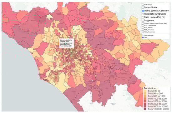
Figure 3.
Representation of the zoning of the Metropolitan City of Rome and population density.
Calibration was carried out using the FCD estimations of trips, stay points, and inter-zonal interactions. As described in the previous section, stay points were extracted by means of a DBSCAN clustering technique [18], which allowed us to classify origins and destinations into the categories “home” (H), “work” (W), and “other” (O). The resulting travel chains enable the extension of the FCD sample to a scale consistent with the circulating vehicle fleet, thereby allowing for the generation of chains tailored to a specific scenario, as illustrated in Figure 4, where an increase in the density of O-D trips can be observed when comparing the FCD sample (about 21k vehicles) with the synthetic one (1.5 M vehicles).
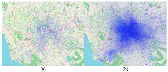
Figure 4.
Origin–destination trips generated from FCD (a) and synthetic (b) samples during the weekday morning peak hour (3 October 2022, 07:00–08:00) across the province of Rome. The synthetic dataset corresponds to a simulated fleet of 1.5 million vehicles (OpenStreetMap contributors, https://www.openstreetmap.org, accessed on 27 November 2025).
By shifting the focus from the classical estimation of aggregated flows between zones (O-D matrices) to a complementary microscale perspective, we can reconstruct the complete sequence of locations visited by each individual over time, thus gaining a deeper understanding of the regularity and variability of private mobility (Figure 5, Table 1). This enables transport policies that are more closely aligned with actual human behavior, allowing for customized analyses, for example, in the context of mobility electrification scenarios.
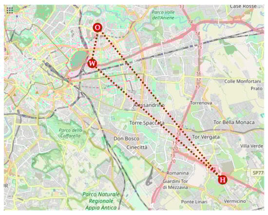
Figure 5.
Example of a home-based trip chain generated through the EPR approach. The sequence of stay points is Home–Work–Other–Home (H–W–O–H), as indicated by the corresponding circles connected with dashed red lines (OpenStreetMap contributors, https://www.openstreetmap.org, accessed on 27 November 2025).

Table 1.
Spatiotemporal information associated with the home-based trip chain shown in Figure 5.
2.3. Energy Consumption Estimation
2.3.1. Electric Cars Energy Consumption for Traction
The evaluation procedures consider the speed-dependent, hot specific energy consumption factor in Equation (1) described in the EMEP/EEA Air Pollution Emission Inventory Guidebook [26]:
where EC is the specific energy consumption (MJ/km); v is the average speed.
The battery electric car curve was obtained by simulating more than 100 driving cycles and was validated using data derived from measurements on a Real Driving Emissions compliant route, with an absolute error of 5.47 Wh/km (deviation of 2.6%) [27].
The curve was differentiated for four car segments distinguished according to motor power (Table 2), using several databases of car models on the market and car registration figures across Europe [28].
Table 2.
Classification of battery electric passenger cars.
The equation parameters for battery electric cars were added in the 2024 updated spreadsheet [29] and are listed in the following table, Table 3:
Table 3.
Parameters of Equation (1) for battery electric passenger cars’ energy consumption calculation.
By comparing the average vehicle consumption curve with the one obtained by ENEA from measurements under real driving conditions, we notice that the difference is below 10% for speeds under 40 km/h, while our measured consumption values are up to 27% lower at higher speeds [30].
2.3.2. Consumptions Related to Heating, Ventilation, and Air Conditioning
Heating, Ventilation, and Air Conditioning (HVAC) consumption can be computed using different approaches. Several studies are devoted to the analysis of specific Heating or Air Conditioning systems, with detailed characterization of the consumption considering the complexity of the vehicle under study [31,32,33,34,35]. Here, we propose a more general, even if less detailed, approach derived from the model proposed by [36,37] for local public transport buses, schematically described in Figure 6.
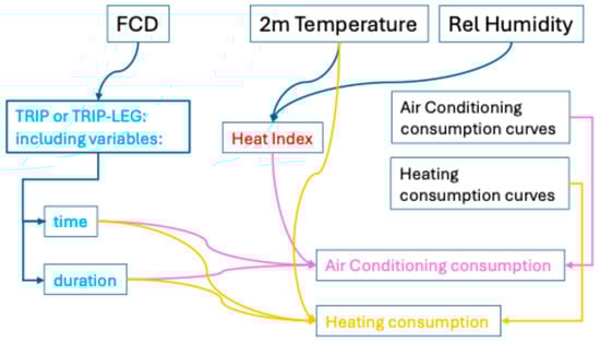
Figure 6.
Scheme of the variables and processes required to compute Heating and Air Conditioning consumption. Variables in black are input variables, variables in red and blue are intermediate variables derived from climatological variables and FCD, respectively, while violet and yellow variables and connections refer to the computation of Air Conditioning and Heating consumption, respectively.
As described above, the information contained in the FCD allows us to reconstruct the exact route of each considered vehicle, particularly the duration of a trip (or a trip leg) and the date and time of departure and arrival. It is therefore possible to compute HVAC consumption, if consumption curves representing the required power for the function of the environmental temperature and humidity are available.
The computation process is slightly different for Air Conditioning and Heating. The most important difference is related to the fact that the Heating system depends only on environmental temperature, while for the computation of Air Conditioning consumptions, humidity must also be considered. Following [36], to avoid a power curve depending on two independent variables difficult to fit with experimental data, we use the Heat Index [38] to include, in only one variable, the influence of both variables. This is not required for the Heating system, whose power curve is well-described in the function of the sole temperature.
The Air Conditioning system is switched off for a Heat Index lower than 20 that corresponds to temperatures close to 20 °C. The Heating system is, in turn, switched off for temperatures higher than 15 °C.
The Air Conditioning system is linear piecewise and defined as
where P is power, HI is the Heat Index, and a and b are coefficients that define the consumption curve and mainly depend on the type of vehicle. This formula can be applied by considering environmental 2 m temperature and Relative Humidity at the time and date of each trip. Energy is then computed by multiplying (integrating) the obtained power by the duration of the trip.
A similar approach is applied for Heating, with only temperature T as the independent variable and a parabolic curve for power:
Meteorological variables are, in general, available from local weather services and do not represent an obstacle to apply this methodology.
Power curves in function of environmental temperature and humidity are the major challenge of the proposed methodology. These curves are empirically derived so that observational campaigns in real operational contexts need to be performed on different kinds of vehicles, with high costs of time, personnel, and instruments. Few works in the literature provide curves for buses, such as, for instance [36,39]. These curves can be adapted to other vehicles by applying a scale factor.
As an example, in Figure 7 we show the power curves for a small city car and a large SUV derived from the curves available for buses used in [37] by applying a scaling factor related to the ratio between the maximum power deliverable by a generic Air Conditioning system for buses (typically of the order of 40 kW) and cars (roughly 4 kW for a small car; 8 kW for a large SUV).
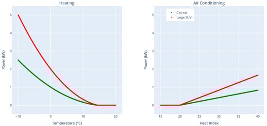
Figure 7.
Left: Power required by the Heating system for a small car and a large SUV in function of environmental temperature. Right: Power required by the Air Conditioning system in function of Heat Index for the same vehicles on the left panel. The curves are derived from the bus curves used in [37] by applying correction coefficients, as described in the text.
2.4. Setting up the Individual Charging Behavior Model in Urban Areas
Electric cars can be charged in various locations and with different power, times, and fares.
For the purposes of modeling charging choices, it is useful to adopt a classification based on charging location:
- At home;
- At intermediate destinations;
- At dedicated service stations.
For each of these location classes, different charging supplies can be available, both in terms of infrastructure ownership (private for exclusive individual use, private for use by a limited community, or public access) and charging characteristics, in terms of power, tariff, occupancy rules, and walking distance to the destination.
These supply characteristics influence the choice of where to charge, along with the characteristics of the associated stopover, particularly the duration, the battery level at the start of the stopover, and the energy requirements for the subsequent charging point.
Efficient design of charging infrastructure requires identifying the factors that mostly influence user behavior [40]. Many authors investigated such a topic, pointing out the role of users’ characteristics [41], travel frequency and mileage [42,43], speed [44,45], and stop duration [46].
The behavioral paradigm adopted for our model is that an electric car user chooses whether to charge for each journey that begins and ends at home, where we suppose that the user always has the option of charging, either via private devices (individual or shared) or via public charging stations located nearby. Furthermore, in urban areas, charging a private car at dedicated service areas is excluded, given a wide availability of charging points near the destinations of the journeys, especially in high population density zones. Figure 8 shows the adopted conceptual behavioral scheme.
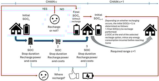
Figure 8.
Conceptual scheme of individual charging behavior built on home-based roundtrips and a bi-level decisional approach.
As illustrated in the previous figure, it is assumed that, for every trip originating from home, the decision-making framework governing vehicle charging operations is structured as a two-tier hierarchical process, encompassing two sequential choices that determine the overall charging strategy, i.e.,:
- Whether or not to recharge during the home-based chain;
- If a positive choice is made at the first level, where to recharge among the available options along the chain.
The decisional process involves a finite number of alternatives for each level of choice and can therefore be modeled using discrete choice models.
The first level of choice can initially be correlated with the following two variables (see the top-right section of Figure 8):
- Expected SOC at the end of the travel chain c, if no recharging is performed.
- Required range in the following chain c + 1, linked to the expected travel distance.
Note that, once the battery capacity (usually expressed in kWh) has been set, the residual range of an electric vehicle can be calculated from the product of the capacity value and the battery’s current SOC over the average consumption of the considered vehicle. Therefore, the probability of charging along a chain c can be expressed as a function of the SOC expected at the end of the chain c and the SOC required for completing the following chain c + 1 or through the correspondent expected/required ranges.
Once an electric vehicle user has chosen to charge during the chain, he must also decide where and when to charge, choosing among the various options available in the chain (see bottom-left section of Figure 8). The following significant attributes for each stop planned during the chain are identified:
- Battery SOC at the start of the stopover, i.e., remaining range based on battery capacity;
- Duration of the stopover;
- Cost of charging (including any additional costs for occupying the charging station beyond the time required for charging, subject to the tolerance margin established by the Operator);
- Charging comfort (which includes the distance of the charging station from the trip destination and the need to move the vehicle to avoid extra costs);
- Battery SOC at the end of the recharge and upon returning home, after completing the chain of trips planned for the day.
Based on the assumption of a two-level choice, we can write the probability that a vehicle will charge during the home-based travel chain c at a certain stop s as a composite probability:
where
- Pc,s is the probability of charging in chain c and at location s;
- δs is a Boolean value indicating whether it is possible to charge an electric vehicle at the stopover (or close to it);
- is the probability that the user will charge in chain c, as a function of the utility value of c;
- is the probability that the user will recharge during stopover s, as a function of the utility value of stopover s.
The utility functions have been set as a linear combination of the choice variables specified above, i.e., as for Uc:
- Vehicle range required for the next-trip chain;
- SOC levels (or equivalent vehicle ranges) when coming back home, if no recharge occurs.
As for Up, the independent variables are
- SOC level arriving at the potential recharge point;
- SOC level at home coming back if the vehicle has been recharged;
- Stopover duration;
- Charging point power and tariff.
Other variables can also be, in principle, included in the second-level utility function to consider possible additional costs if the vehicle is not removed from the charging point as soon as the recharge is concluded (unauthorized occupancy penalty), as well as comfort factors, such as walking distance from the charging point to the trip destination.
Both utility functions’ forms and coefficients have been defined and calibrated based on the results of the survey described in the following section, enabling authors to also include other kinds of variables other than strictly utility-based, such as socio-economic, behavioral (mobility), and possible psycho-attitudinal aspects.
2.5. Survey for Individual Charging Choice Model Calibration and Main Calibration Results
To verify the actual role of first- and second-level choice variables, an SP survey was conducted to record declared charging behaviors in relation to different scenarios.
The SP survey technique involves presenting respondents with various travel situations, battery conditions, and characteristics of available charging points (“scenarios”), offering them a choice from a limited set of alternatives [47].
To ensure a sample sufficient to represent the future population of BEV owners/users and not influenced by current charging behaviors, which could be affected by a context not yet fully adapted to the widespread use of battery-powered electric vehicles (early adoption), the survey was also extended to a class of users with no charging experience.
In the paradigm adopted for charging behavior (see Section 2.4), the first-level choice intrinsically involves selecting between only two alternatives: immediate or postponed charging, based on the ratio between the range available upon returning home in the event of a lack of charging and the range required for travel until the next homecoming. Thanks to this intrinsic simplicity, it was not necessary to introduce simplifications in the survey questionnaire.
The second-level choice, on the contrary, can theoretically involve more than two alternatives, depending on the number of intermediate stops planned during the home-to-home travel cycle. For better questionnaire readability, the second-level choice was proposed for a simple travel chain, i.e., with only one intermediate stop along the home-to-home route. In practice, respondents were asked to choose between the options “charging at the intermediate destination” and “charging upon returning home,” varying the combination of values of the choice variables hypothesized for each alternative. When applying the model to residents’ mobility patterns, the binary choice was reduced where necessary to multiple alternatives under specific behavioral assumptions (see Section 2.6).
Based on the set of the most significant variables in the charging choice process and their respective ranges of variation (see the following table), the University of Salerno (UNISA), by combining first- and second-level choice situations, identified 138 significant investigation scenarios to calibrate the choice model.
Table 4 shows the ranges of the scenarios’ variables, the combination of which resulted in 138 significant scenarios.
Table 4.
Choice variables and related ranges.
Given the complexity of the situations to be presented to the respondents, it was decided to limit the number of scenarios to two for each questionnaire, resulting in 69 questionnaire formats. For each of these, it was necessary to ensure a statistically significant sample of interviews.
Participation in the survey did not require prior experience in driving or charging battery electric vehicles but only the possession of a valid driver’s license. For this reason, access to the questionnaire was preceded by an animated tutorial designed to provide essential knowledge, ensuring informed responses.
The survey, which involved multiple stakeholders in the dissemination of the questionnaire, recorded nearly 10,000 accesses. However, only 6800 participants completed the form up to the socio-economic profile section, and fewer than 6000 responded to the optional psycho-attitudinal questions located at the end of the questionnaire. Despite this relatively high dropout rate (30%), the target of at least 100 valid responses for each of the 69 questionnaires administered was successfully achieved.
The valid sample represents 0.021% of the Italian population holding a driver’s license—a percentage that is not fully representative of the reference population but, nonetheless, is highly significant in absolute terms when compared to similar research efforts conducted globally.
As shown in Figure 9, Northern and Central Italy are the most represented geographical areas, with only 20% of respondents coming from Southern Italy. In terms of gender, most participants are male (57%), while the youngest (18–24) and oldest (>65) age groups are the least represented. Only a small number of respondents reported familiarity with electric vehicles. These imbalances partially reflect the actual demographics of licensed drivers in Italy.
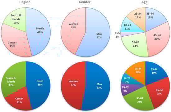
Figure 9.
Overall demographic distribution (by geographic region, gender, and age) of the SP survey sample (top) in comparison with driving licenses in Italy (down).
Before calibrating the model, post-stratification and weighting were applied by comparing the sample’s demographic distribution with census data. Both decision levels—whether to charge and where/how to charge—were modeled using a Multinomial Logit Model (MNL), calibrated through weighted maximum likelihood estimation. Some details can be found in [48,49], while a deeper insight is being submitted by research partners of UNISA for a further scientific paper [50].
In the very essence, the utility functions resulting from calibration process for the first-choice level alternatives are based on eight attributes, four of which relate to individual characteristics.
For the second-level choice, the model considers thirteen significant attributes, four of which are related to individual characteristics.
The decision to charge an electric vehicle during a travel chain is mainly influenced by the vehicle’s SOC, remaining range, and the distance to be traveled the next day. The choice of charging location is primarily affected by charging costs and total expenses, followed by proximity to the destination, battery level to be recharged, and stop duration. Socio-demographic factors like gender, age, driving frequency, and daily distance also play a role.
2.6. Behavioral Model Application to the FCD Format
The model is intended to be applied to the residents’ mobility patterns by private car, reconstructed as specified in previous Section 2.2 and Section 2.3.
Based on the behavioral model structure, travel stopovers are classified into “Home” and “Others”, including stops at work into the “Others” class.
To apply the model, it is necessary to associate the values of the variables that define the individual profiles for the following aspects:
- Characteristics of the electric vehicle used;
- Gender and age group;
- Mobility intensity in a typical week.
In the absence of verified information on the above topics in the FCD format, some criteria to associate model attributes to individuals have been assumed.
Each individual is assigned a battery capacity (kWh) associated with the maximum estimated consumption for the most energy-intensive travel chain detected over a sufficient monitoring/simulation period. Each battery size is associated with a maximum charging power (kW) and a maximum expected range (km) when the battery is fully charged (SOC = 100%).
Gender and age group are assigned using random processes based on the statistical distributions of the driving license population in the study area.
The mobility variables are directly derived from the travel patterns associated with each individual.
At the same time, it is necessary to define a charging infrastructure penetration scenario that provides the following information for each stop:
- The nominal charging power (kW) of the charging points available at each stop; in the charging process simulation, the actual power used is the lower of that of the charger and that absorbed by the battery;
- The charging fare, which will be associated with the power supplied and the type of stopover location (home, other);
- Walking distance from the charging point to the destination; here too, a distinction is made between charging at home and charging at other destinations.
Once the individual profile and charging characteristics for each stopover have been defined, the charging decision is based on the values of the variables deduced directly or indirectly from the FCD format, namely: stopover duration, SOC (at the start of the stopover and at the end of the day if not charging), and the range required for the immediately subsequent trips.
A common problem faced when modeling electric vehicle routines is SOC initialization. Here, we propose adopting the more flexible approach proposed, for example, in [51,52], in which multiple consecutive days are simulated until periodic SOC behavior is obtained. On the first day of the simulation, all EVs depart with fully charged batteries. The same routes are performed for three consecutive days or until the initial SOC becomes insensitive to the one chosen for the first day. The SOC thus obtained is the initial one for the simulation of the period under consideration.
The sequential procedure, starting from the first time leaving home to the last time to come back in a certain analysis period (e.g., a typical workweek), calculates the following:
1. For each travel chain carried out in the period, the probability that a charge occurs;
2. For each detected/simulated stop at the destinations of the travel chain (including coming back home), the probability that the provided charge occurs at that location and at that clock time.
The first-level utility functions (“Recharge” or “No-recharge”) are computed based on the individual’s vehicular, mobility, and socio-economic attributes, along with the residual SOC and remaining driving range at the end of the chain without recharging. These values are then compared to the required range for the subsequent chain. By combining the two utility values, corresponding choice probabilities were derived.
A Monte Carlo (MC) simulation is then applied to assign to each chain one of the two first-level alternatives: recharge or no recharge. In this simulation, the recharge option is excluded for chains with a recharge probability less than or equal to 30%. This assumption effectively limits simulation of recharge occurrences when the SOC and range upon returning home are likely sufficient to meet future mobility needs.
It should be noted that several travel chains consist of a single trip. This outcome is attributable to the methodological choice of including only those trips whose final stop duration is equal to or greater than 30 min. Consequently, in real-world scenarios, these ‘chains’ may encompass intermediate destinations whose stop durations are too brief to be considered viable for charging opportunities, given the standard urban charging power levels. Nonetheless, such specific travel chains may still require charging upon returning home due to a low initial SOC, a substantial total distance traveled, or a combination of both factors. For these chains, the probability of charging is significantly lower than for multi-trip chains, yet it is not negligible. In these cases, whenever the Monte Carlo simulation identified a charging event, the operation was naturally assigned to the home location.
In all other cases, when the first MC simulation indicates a “Recharge” choice, a second-level simulation is performed to determine the preferred location: home or other destinations. Utility and probability values are calculated using the attributes defined by the UNISA model, including charging tariff, total cost, and walking distance for both options, stop duration and initial SOC at other destinations, final SOC at home after destination charging, difference between final SOC at home for the two options, and the individual’s socio-economic and mobility profile.
For complex travel chains, i.e., those involving more than one intermediate destination, the binary choice model is applied by selecting the destination with the highest utility function value with respect to the home alternative.
Following Monte Carlo simulations, charging events are determined and, for each of them, the power used, the starting time, and the duration until full charge or scheduled departure. This data is used to generate probabilistic charging profiles for each urban zone over the simulation period, with statistical reliability increasing with the number of events per zone, as specified in the subsequent flow chart (Figure 10).
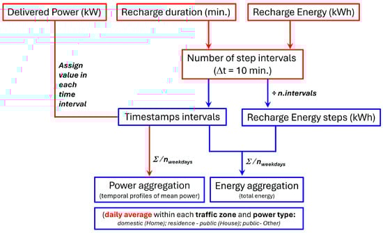
Figure 10.
Procedure to estimate total delivered charging power by traffic zone and fixed time intervals as implemented in the algorithm to compute recharge data aggregation.
The profiles are implemented at time intervals of ten minutes to follow the users’ charging behaviors. For this purpose, the number of ten-minute intervals occurring for each recharge process is computed. While the energy recharged has been equally spread over the whole duration of the recharge, the delivered power is kept constant within each time interval. On the other hand, hourly power profiles are computed considering the spatial-temporal aggregations of charging events. Practically, all energy contributions are aggregated (summed) within each time interval and within each traffic zone.
3. Results
3.1. Case Study—Demand and Offer Qualification
For research purposes, the proposed procedure has been applied using a set of FCD collected by Viasat in the metropolitan area of Rome during the period October–November 2022. This dataset was provided by Roma Mobilità Agency and processed by ENEA and its academic research partners during the three-year research activities to feed the entire modeling suite developed for urban mobility analysis, including the module for estimating the charging profiles under discussion.
The complete dataset comprises approximately 20,000 vehicles, but only for a subset—around 11,500—was it possible to infer a likely residence within the study area. From this subset of “resident” vehicles, those with a mobility not sufficient to define a reliable charging behavior were excluded, as well as those whose mobility patterns suggested usage not attributable to individuals or small households but rather to commercial purposes (e.g., taxis, car sharing, goods distribution, etc.). After filtering out non-eligible terminals, the final sample suitable for applying the charging model consisted of approximately 8700 vehicles.
The model was applied to the full set of these 8700 agents under the assumption that they represent fully electric vehicles (BEV). Based on this assumption, the sample corresponds numerically to approximately 40% of the BEV fleet registered in the Province of Rome as of 31 December 2023, according to data from the National Unified Platform (PUN) for charging infrastructure (https://www.piattaformaunicanazionale.it/, accessed on 2 November 2025).
The sample includes nearly 460,000 home-based trip chains, with approximately 225,000 intermediate destinations. This discrepancy arises from the fact that many reconstructed chains are loops from home to home without intermediate stops due to the concatenation of trips separated by stops shorter than 30 min—considered the minimum duration for a meaningful charging event. For such loops, only the first-level choice model is applied, while the second-level model is not. Conversely, numerous “long” chains exist, containing more than one intermediate destination, which will be analyzed in detail in the results section of the charging model application.
For each eligible individual in the sample, mobility attributes required by the behavioral model were computed based on the two-month observation period. The resulting statistical frequencies are reported in Table 5, showing the average number of travel days per week and the average daily distance on working days. It is observed that most sampled individuals use their private vehicle more than three days per week, while in terms of daily mileage, most travel less than 60 km per day—especially among those who use their vehicle more frequently.
Table 5.
Distribution of mobility attributes required by the charging model on the FCD sample.
To better verify the outcomes of the modeling application, the attributes of gender and age—randomly assigned to the FCD application sample (which originally lacks them)—replicate the statistical distribution observed among respondents to the SP survey, limited to licensed individuals residing in metropolitan areas. As a result, the attribute “female_gender” accounts for approximately 43% of the individuals, while around 60% fall within the age range of 45 to 75 years (Table 6).
Table 6.
Assumed distribution of gender attribute on the FCD sample.
The electric vehicle size was assigned to each sampled individual based on the maximum cumulative energy consumption observed across their trip chains. Specifically, 50% of the sample was assigned a small-sized electric vehicle (40 kWh battery, nominal range of 220 km), 43% a medium-sized vehicle (50 kWh battery, range of 280 km), and 7% a large-sized vehicle (70 kWh battery, range of 370 km).
These modeling assumptions tend to favor the selection of vehicles with smaller battery capacities, aligned with typical urban mobility needs, while penalizing larger battery configurations. Naturally, in commercial analyses, these assumptions could be adjusted to better reflect the actual composition of the electric vehicle market.
Each battery size has been associated with one of the electric car dimensional categories of the EMEP/EEA methodology for energy consumption calculation (see Section 2.3.1), excluding the “mini” type.
The initial SOC was set to 100% for all vehicles at the beginning of the simulation. This choice was made feasible by the extended observation period, which allows for averaging daily charging profiles over multiple days, thereby minimizing the impact of assumptions regarding the initial SOC level.
As for the charging supply, the behavioral model was applied to two distinct scenarios, defined based on specific technical parameters.
Scenario 1 (s1): This scenario serves as the Reference Case, incorporating assumptions considered realistic in the near future. In fact, it includes both private (home) and public charging options, reflecting a plausible configuration of charging availability and infrastructure deployment.
Scenario 2 (s2): This scenario was designed to test the behavioral model under simplified assumptions, particularly aimed at minimizing the influence of charging costs in comparison to alternatives. The primary objective was to assess the model’s sensitivity to cost-related variables by comparing results obtained under s1 and s2.
Table 7 summarizes and compares assumptions made on charge infrastructure characteristics for both scenarios, while the following discussion elaborates on the decomposition of power and cost ranges.
Table 7.
Charging infrastructure characteristics across the two simulation scenarios.
In s1, for 50% of the population, the availability of home charging was assumed.
The domestic charging power was calibrated based on the battery capacity of the electric vehicle, as listed below.
- 40 kWh Battery 3.6 kW;
- 50 kWh Battery 7.2 kW;
- 70 kWh Battery 11.0 kW;
This assumption reflects a realistic distribution of home charging capabilities, considering possible residential power availability and the technical requirements of different EV models.
Charging tariffs were defined considering the following: a. charging location (home or other destinations), b. charging accessibility (restricted or public), and c. charging power (3.6 ÷ 11 kW).
The specific tariffs used in s1 are highlighted in Table 8. These values were selected to reflect realistic cost conditions for the reference scenario.
Table 8.
Electricity tariffs by location, accessibility, and power in s1.
The walking time to public charging stations near the residence was set to 5 min, based on the hypothesis that proximity to charging infrastructure may positively influence the willingness to purchase an electric vehicle in the absence of private charging options.
For public charging at other destinations, walking time was determined based on the surface area of the corresponding zone, according to the following rule (Table 9):
Table 9.
Walking time vs. zone area.
The analysis considered a total of 1322 traffic zones, with the distribution of walking times illustrated in Figure 11.
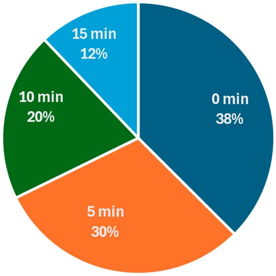
Figure 11.
s1—walking time distribution for public recharge at other destinations than home.
In s1, no penalty was applied for extra-time parking at public charging stations located near the residence. However, for public charging at other destinations, a penalty of EUR 0.09 per minute was applied for delays exceeding 60 min, with a maximum charge of EUR 6.
As for s2 infrastructural characteristics, it is assumed that no home location has domestic recharge and all public charging stations were assigned a uniform power level of 11 kW and a flat tariff of EUR 0.60/kWh.
The walking time to access public charging stations was standardized to 5 min for all public charging events, regardless of whether the location was near the residence or at other destinations and no penalties were applied for improper parking at any public charging location.
3.2. Case Study—Simulation Results
3.2.1. Aggregate and Individual Charging Behavior
According to the behavioral model results for our case study, the likelihood of recharging increases with the number of stops within the home-based roundtrip, reflecting the cumulative energy consumption. The trend is consistent across both analyzed scenarios, with a slightly higher probability in s2, where recharging at the destination is more frequent. This leads to lower initial SOC levels in subsequent chains compared to when recharging occurs at home, which is more common in s1.
Figure 12 presents the results of the first-level choice simulation for both scenarios, showing the frequency of recharging among chains with a recharge probability above 30%.
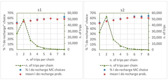
Figure 12.
Frequencies of “Recharge” choices from the MC simulation for all home-based chains with recharge probability >30%, compared to average modeled probabilities. s1 (left) and s2 (right).
The outcomes are largely consistent between the two scenarios, except for the longest chains, where randomness has a greater impact due to the smaller sample size.
The average probability of selecting “Destination” varies significantly between the two scenarios, highlighting the model’s sensitivity to assumptions regarding charging infrastructure availability (public and private), power levels, and costs (Figure 13).
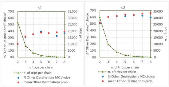
Figure 13.
Frequency of “Destination” selections following the second-level choice MC simulation, compared to average modeled probabilities. s1 (left) and s2 (right).
In s2, where tariffs and walking distances are equal for both destination and home, the model estimated an average “Destination” choice probability of approximately 50% among chains where the first-level choice was “Recharge.”
In s1, where tariffs and walking distances favored home charging, the “Destination” choice probability dropped to 20% for chains with a single intermediate destination, reaching a maximum of 40% for chains with four destinations.
The second-level simulation results (Figure 13) closely align with the average probability values, except for chain length categories with limited sample sizes. Notably, a larger deviation is observed between the simulated choice frequency and the average probability for the second-level choice than the first-level choice, primarily due to the smaller sample size.
In both scenarios, a slight positive correlation is observed between first-level and second-level choice probabilities: the average probability of selecting “Destination” increases when the probability of choosing “Recharge” is higher. Conversely, when the probability of “No Recharge” is higher, the likelihood of selecting “Destination” decreases.
Table 10 summarizes the aggregated results of the recharge model applied to the Rome case across the two infrastructure scenarios in terms of the following: average probability of the “Recharge” choice of all 456,832 chains (avg_p_yes), share of choice “Recharge” of the chains with a probability higher than 30% after MC simulation (% MC = yes, p_yes > 30%), average probability of the “Destination” choice of all 437,544 intermediate destinations (avg p_dest); average probability of the “Destination” choice of intermediate destinations when the MC first-level choice is “Recharge” (avg p_dest, MC = yes), and share of the “Destination” choice when MC first-level choice is “Recharge” (% MC = dest, MC = yes).
Table 10.
Main results of behavioral model application and MC simulations.
Table 11 and Table 12 present aggregate simulation results based on battery capacity, respectively, at home and at other destinations. Scenarios and battery size comparisons are based on the average initial SOC, average final SOC, and average recharged energy.
Table 11.
Home recharging habits based on battery capacity.
Table 12.
Other destinations recharging habits based on battery capacity.
Initial SOC levels for home charging are generally lower than those for destination charging, with average values of approximately 35% and 39%, respectively, across both scenarios.
As battery capacity increases, the initial SOC at the start of charging tends to rise. Although this may appear counterintuitive—given that a 70 kWh battery at 40% SOC still offers substantial range—it is partially supported by the results in Figure 2, which show that a notable share of users chooses to recharge even with a high residual range relative to the next trip.
Final SOC levels are typically higher for home charging than for destination charging (94% vs. 83%/76%), with a slight downward trend for larger batteries. Energy delivered during home charging is significantly greater than at destinations, increasing proportionally with battery capacity.
Additionally, the average duration of charging stops ranges from approximately 15.6 h in s1 to 11.9 h in s2.
Home charging, more prevalent in s1, benefits from longer stop durations—not only because home stops are inherently longer, but also because the behavioral model tends to favor shorter destination stops, which result in lower overall charging costs where tariffs are higher.
As an example, Figure 14 shows the trend of the battery SOC simulated for a car with a 40 kWh battery over more than 60 travel chains during the two-month analysis period. For this vehicle, s1 includes access to private home charging, which is unavailable by default in s2.
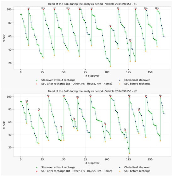
Figure 14.
SOC trend over the two-month analysis period for a vehicle with a 40 kWh battery. s1 (top) and s2 (down). Initial SOC at every stopover is shown, distinguishing among type of stop location: home (Hm), intermediate destination (Ot), and public recharge near home (Hs). Stopovers without any recharge event are depicted in green while stopovers with a recharge event are depicted in yellow for the SOC before the recharge and in red as for the SOC after the recharge. Stopovers ending a chain (at home or nearby) are evidenced in black.
Going from s1 to s2 reveals a clear shift from home charging to charging at other destinations.
In s1, the vehicle performs 12 charging events, 11 of which occur at home, almost always resulting in a full recharge. Only toward the end of the period does a full recharge occur at an intermediate destination, followed by a top-up (“biberonage”) at another destination to avoid battery depletion after two energy-intensive chains.
In s2, the total number of charging events increases to 15, resulting in a slightly higher final SOC than in s1. Seven of these charges occur at intermediate destinations, mostly as partial charges.
Enlarging the vision to other individual samples, and also to varying battery size and recharging infrastructure availability and characteristics, it emerges that the behavioral model performs more realistically when charging tariffs discourage the “Destination” option, which otherwise tends to be selected too frequently.
This finding suggests the need for adjustments to the model to limit unnecessary top-ups (“biberonage”), which may not always be justified.
In all analyzed cases, Scenario 2 shows an increase in the total number of charging events, along with a higher incidence of recharges at intermediate destinations—exceeding 50% for the vehicle with the smallest battery capacity.
As previously observed in the overall results, this outcome is primarily due to the equalization of charging tariffs between the home and destination assumed in this scenario. Despite this tariff alignment, the total cost of charging tends to be higher at home, where the average amount of energy delivered is greater. This is driven by two concurrent factors: a lower initial SOC at the start of charging and a longer available time window to complete the recharge.
In s1, both the total number of charging events and the share of those occurring at intermediate destinations decrease. In this scenario, the cost of charging at destinations is significantly higher than in s2 and, more importantly, higher than at home—even when private home charging is unavailable.
Charging costs at intermediate destinations rise in s1 due to both higher tariffs and the application of an additional fee for overstaying at the charging station beyond the required time (plus a 60 min tolerance).
Overall, unit charging costs tend to converge across the two scenarios. s1 is penalized by higher destination tariffs but benefits, in some cases, from the presence of private home stations where lower rates apply compared to public home charging—the only option available in s2.
Previous graphs express the maximum detail of simulations, from which aggregate estimates on energy demand over time and space are derived, as shown in the subsequent paragraph.
3.2.2. Charging Profiles
Daily average of recharged energy (kWh) and delivered power (kW) required within each traffic zone per weekday has been computed considering outputs for the whole month of October 2022. For the sake of clarity, the same number of weekdays were considered to compute daily averages.
In summary, for each weekday and a traffic zone, power profiles referred to the mean/maximum power. Within the same time interval, charging contributions can be of different power types, such as domestic (home), public near the user’s residence (House), or public near to other stay points (other).
Analysis of full-electric private cars’ charging demand during the week shows that from Wednesday to Friday the charging activity is higher compared to other days of the week, especially on Friday. Instead, the weekend is characterized by a drop, with Sunday being the day with the lowest charging activity. On the other hand, the days Monday and Tuesday show relatively high charging activity, indicating a gradual increase after the weekend.
The charts shown in Figure 15 and Figure 16 illustrate the estimated hourly trend of average power demand across the entire study area on a representative Wednesday for both analysis scenarios.
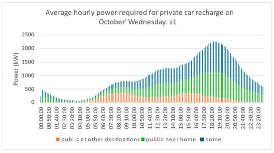
Figure 15.
Average charging power demand across the metropolitan area of Rome on Wednesdays under analysis—s1.
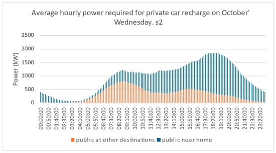
Figure 16.
Average charging power demand across the whole metropolitan area of Rome on Wednesdays under analysis—s2.
The above Figure illustrates the role of the different components of power demand in both scenarios. Charging at intermediate destinations exhibits a dual peak pattern—one in the early morning hours and another in the afternoon—whereas home-based charging shows a pronounced peak during evening return hours and a secondary peak in the early afternoon, coinciding with a decline in charging activity at other destinations.
In s2, power demand is more evenly distributed throughout the day. This is due to the increased cost competition between home-based charging and charging at alternative destinations. The latter tends to occur predominantly in the morning and afternoon, while the former remains concentrated in the evening.
In both scenarios, there is a near-complete drop in power demand between 2:00 a.m. and 5:00 a.m. This observation highlights the potential for implementing load-shifting strategies through targeted pricing policies and/or smart charging techniques to optimize energy demand distribution over time.
Figure 17 presents the trend of absolute peak power values observed at different hours of the day throughout the entire month of analysis. In practice, the below histograms represent the envelop of the daily trends during the considered period. When referred to specific zones, as can be done by subdividing the territory into suitable sub-areas, these outputs are of critical importance for assessing the adequacy of the electrical grid supporting the charging infrastructure.
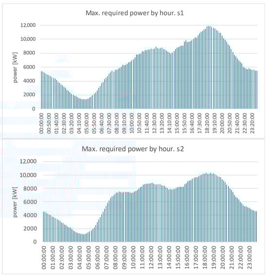
Figure 17.
Max. required power by hour in the analysis period—s1 (up) and s2 (down).
The trend of peak power values over the analysis period qualitatively confirms the patterns observed in the average power profiles presented earlier. Comparing these two metrics provides valuable insights into developing strategies to manage electricity demand and supply.
Based on the simulated power demand and assuming no congestion effects, the total installed power capacity required to meet charging needs—both private and public—is estimated as follows:
- 53,198 MW in s1;
- 22,178 MW for private charging infrastructure;
- 31,020 MW for public charging infrastructure;
- 42,224 MW in s2, entirely allocated to public charging infrastructure.
By aggregating individual charging behaviors, it is also possible to estimate the minimum number of charging points required in each zone to satisfy the simulated charging demand at any time during the analysis period, assuming no demand-side management strategies (e.g., smart charging). This enables a preliminary estimation of the investment requirements for both private and public charging infrastructure based on unit cost assumptions.
4. Discussion and Conclusions
The methodology proposed is grounded in the use of FCD, which offers the distinct advantage of being applicable across diverse territorial contexts, if vehicle monitoring is sufficiently widespread. This monitoring is primarily driven by insurance-related purposes, as insurance companies benefit from tracking events that involve damage compensation, thereby enabling reductions in insurance premiums.
In Italy, a significant proportion of vehicle owners have adopted this technology, resulting in a relatively high penetration rate of onboard monitoring devices—currently estimated at approximately 18% of all mandatory motor insurance policies [53].
In addition, the European Parliament, within the framework of the “Vision Zero” strategy aimed at eliminating road fatalities by 2050, has recently enacted Regulation GSR 2019/2144. This regulation mandates the installation of On-Board Units in all vehicles registered from 2024 onwards, specifically for accident detection. Although access to monitoring data is restricted to competent authorities and only permitted in cases of serious accidents, the regulation is expected to further encourage the continuous monitoring of private mobility. This would significantly enhance the understanding of mobility dynamics and improve the effectiveness of policies promoting sustainable transport demand management at local, regional, and national levels.
In this evolving landscape, the development of digital platforms capable of storing and processing FCD samples is accelerating. These platforms also provide advanced analytical and simulation tools that are highly valuable for transport system planners and operators. In this context, a web-based mobility platform PRIORITY (Platform for the tRansition to sustanInable zerO-caRbon mobilITY) is going to be developed by ENEA to support the mobility governance processes, oriented toward energy efficiency. This platform has the purpose of innovating the knowledge and evaluation processes of urban mobility by offering a relevant instrument to mobility managers to design Sustainable Urban Mobility Plans (SUMPs).
Nonetheless, the use of FCD for analytical purposes presents several critical limitations.
First and foremost, privacy regulations—specifically EU Regulation 2016/679 (GDPR)—impose strict constraints on the use of personal data that could directly or indirectly identify individuals. The European Data Protection Board (EDPB) guidelines require the implementation of specific safeguards such as anonymization and pseudonymization. While these measures are generally adopted by FCD providers, a recent requirement to continuously change vehicle ID code may significantly hinder the reconstruction of individual mobility patterns over extended timeframes.
Another key concern is the statistical representativeness of the FCD sample relative to the target population, which must be rigorously validated prior to conducting any analysis.
Furthermore, FCD is typically provided on a commercial basis, necessitating the allocation of a dedicated budget for its use in analytical methodologies. Ideally, this budget should also encompass access to enriched datasets beyond the standard FCD format, which typically categorizes vehicles into two broad groups: Light-Duty Vehicles (LDV) and Heavy-Duty Vehicles (HDV). Possible additional data—compliant with privacy regula year of registration), predominant usage (private, corporate, and commercial), and the territorial scope of short-range circulation (e.g., inferred from the administrative area of the insurance contract). Such supplementary information would support the assignment of scenario variables related to vehicle size class, demographic characteristics of the primary user, and area of residence.
Similarly, a more comprehensive and detailed knowledge base regarding the distribution and characteristics of urban charging infrastructure, particularly private charging points (individual or shared within residential buildings), could facilitate the definition of baseline scenarios for charging supply. These baselines would serve as reference points for evaluating potential infrastructure expansion, especially in geographic areas such as Italy, where the adoption of electric vehicles remains relatively modest.
With respect to traction energy consumption estimation, the methodology employed is well-established and has long been utilized in the development of regional inventories for road transport energy use and emissions. However, it is noted that this model is suitable for large-scale or real-time applications, providing good results, since it requires fewer data input and enables fast processing [27,54].
The estimation of energy consumption attributable to cabin climate control (heating and cooling) is based on an original procedure developed by ENEA. This procedure currently relies on measurements taken from electric buses, with additional campaigns underway. A dedicated study focusing on passenger cars is planned, involving the development of curves that describe HVAC system power requirements as a function of ambient temperature and humidity based on experimental or simulated vehicle cabin conditions. These findings will be presented in future publications. Preliminary results from an analysis of HVAC consumption in the ATAC fleet in Rome indicate that, under the most severe climate change scenarios outlined by the IPCC for the remainder of this century, HVAC-related energy demand could significantly affect both charging requirements and range estimates for electric vehicles. In summer, peak HVAC energy demand could reach up to 40% of the total traction energy. These impacts may be partially mitigated by anticipated improvements in battery efficiency and charging technologies.
In conclusion, despite the lack of certain key data required for scenario definition in the case study, the proposed methodology has demonstrated its effectiveness as a predictive tool for urban electric vehicle charging power demand across simulation scenarios, as illustrated by the charging profiles resulting in the two case studies examined (Figure 17).
Through our procedure, each demand/supply scenario can be evaluated in terms of the hourly distribution of peak charging power demand at the level of individual urban zones or across broader areas, thereby informing potential upgrades both to the recharge infrastructure and electricity distribution network.
Moreover, simulation results enable downstream analysis to estimate the financial investment required for public and private charging infrastructure, as well as the impact on charging costs for electric vehicle users.
Finally, the potential for smart charging and Vehicle-to-Everything (V2X) applications can also be assessed. Future developments will include distinguishing corporate charging supply and evaluating the impact of potential queuing during peak demand periods.
To better validate the proposed methodology, waiting for actual data from the field, another predictive behavioral module is now being developed using results of a Revealed Preferences (RP) survey. The new model estimates recharging probabilities through the analysis of the conditional probabilities statistically emerging from the revealed behavior of the electric vehicle users. The next research activities will provide a comparison between methodologies and results of the two analytical approaches, involving recent external research findings on the same subject.
Author Contributions
Conceptualization, M.P.V.; methodology, V.C., M.C., A.G., C.L., G.V., and M.P.V.; software, V.C., A.G., F.K., and C.L.; formal analysis, V.C., M.C., A.G., M.L., C.L., G.V., and M.P.V.; investigation, V.C., M.C., A.G., M.L., and C.L.; data curation, M.C., A.G., F.K., and C.L.; writing—original draft preparation, M.P.V.; writing—review and editing, V.C., M.C., A.G., F.K., M.L., C.L., G.V., and M.P.V.; visualization, V.C., M.C., F.K., and C.L.; supervision, G.V. and M.P.V. All authors have read and agreed to the published version of the manuscript.
Funding
This work was carried out within the framework of the 2022–2024 Three-Year Plan of the National Electric System Research, funded by the Italian Ministry of Environment and Energy Security (https://www.mase.gov.it/portale/-/ricerca-di-sistema-elettrico-nazionale-1, accessed on 23 October 2025).
Data Availability Statement
FCD were provided by Roma Servizi per la Mobilità (https://romamobilita.it/it, accessed on 23 October 2025) and cannot be publicly shared. Aggregate anonymized information can be obtained by contacting the authors.
Acknowledgments
The authors wish to thank Roma Servizi per la Mobilità (https://romamobilita.it/it, accessed on 23 October 2025) for providing the core data for this research. Special thanks to the UNISA research partner for the behavioral model development and valuable support to define SP survey scheme.
Conflicts of Interest
The authors declare no conflicts of interest.
Abbreviations
The following abbreviations are used in this manuscript:
| ATAC | Azienda per la mobilità di Roma Capitale s.p.a |
| BEV | Battery Electric Vehicle |
| DSS | Decision Support System |
| EPR | Exploration and Preferential Return (model) |
| FCD | Floating Car Data |
| HVAC | Heating Ventilation and Air Conditioning |
| IPCC | Intergovernmental Panel on Climate Change |
| MC | Monte Carlo (simulation) |
| MNL | Multinomial Logit Model |
| OBU | On-Board Unit |
| OD | Origin-Destination |
| RP | Revealed Preferences (survey) |
| RSM | Roma Servizi Mobilità |
| SOC | State of Charge (battery) |
| SP | Stated Preferences (survey) |
| UNISA | University of Salerno |
| V2x | Vehicle to Everything |
References
- Dharangaonkar, S.K.; Patil, S.A. Planning of electric vehicle charging infrastructure: A review and a conceptual framework. Int. J. Sustain. Dev. Plan. 2025, 20, 2317–2330. [Google Scholar] [CrossRef]
- Brady-Phillips, V. Scaling Investment in EV Charging Infrastructure. World Economic Forum. 2024. Available online: https://www3.weforum.org/docs/WEF_Scaling_Investment_in_EV_Charging_Infrastructure_2024.pdf (accessed on 23 October 2025).
- Ferwerda, R.; Roldan, J.D.; Khamrakulova, N.; Janssens, R. E-Mobility Compendium. United Nations Economic Commission for Europe. 2025. Available online: https://unece.org/sites/default/files/2025-04/Draft%20Compendium%2021032025.pdf (accessed on 23 October 2025).
- Hall, D.; Lutsey, N. Electric Vehicle Charging Guide for Cities. International Council on Clean Transportation. 2020. Available online: https://theicct.org/sites/default/files/publications/EV_charging_guide_02262020.pdf (accessed on 23 October 2025).
- Joseph, Z.S.; Anosike, A.C.; Adegboyega, B.A. Integration of EV charging infrastructure into smart buildings. IOSR J. Mech. Civ. Eng. 2025, 21, 38–44. [Google Scholar] [CrossRef]
- Andrenacci, N.; Valentini, M.P. A literature review on the charging behaviour of private electric vehicles. Appl. Sci. 2023, 13, 12877. [Google Scholar] [CrossRef]
- Carrese, S.; Cipriani, E.; Mannini, L.; Nigro, M. Dynamic demand estimation and prediction for traffic urban networks adopting new data sources. Transp. Res. Part C Emerg. Technol. 2017, 81, 83–98. [Google Scholar] [CrossRef]
- Busillo, V.; Gemma, A.; Cipriani, E. Simulation-Based Aggregate Calibration of Destination Choice Models Using Opportunistic Data: A Comparative Evaluation of SPSA, PSO, and ADAM Algorithms. Future Transp. 2025, 5, 118. [Google Scholar] [CrossRef]
- Wang, P.; Lai, J.; Huang, Z.; Tan, Q.; Lin, T. Estimating traffic flow in large road networks based on multi-source traffic data. IEEE Trans. Intell. Transp. Syst. 2021, 22, 5672–5683. [Google Scholar] [CrossRef]
- Othman, B.; De Nunzio, G.; Laraki, M.; Sabiron, G. A novel approach to traffic flow estimation based on Floating Car Data and road topography: Experimental validation in Lyon, France. In Proceedings of the IEEE 25th International Conference on Intelligent Transportation Systems (ITSC), Macau, China, 8–12 October 2022; pp. 2571–2576. [Google Scholar] [CrossRef]
- Cipriani, E.; Gemma, A.; Nigro, M. A bi-level gradient approximation method for dynamic traffic demand estimation: Sensitivity analysis and adaptive approach. In Proceedings of the 16th International IEEE Conference on Intelligent Transportation Systems, The Hague, The Netherlands, 6–9 October 2013. [Google Scholar] [CrossRef]
- Lazzeroni, P.; Caroleo, B.; Arnone, M.; Botta, C. A Simplified Approach to Estimate EV Charging Demand in Urban Area: An Italian Case Study. Energies 2021, 14, 6697. [Google Scholar] [CrossRef]
- Melis, A.; Pisano, G.; Pilo, F.; Ruggeri, S. A model for estimating the energy demand of the EV charging stations in an urban area. In Proceedings of the 2023 IEEE International Conference on Environment and Electrical Engineering and 2023 IEEE Industrial and Commercial Power Systems Europe (EEEIC/I&CPS Europe), Madrid, Spain, 6–9 June 2023; pp. 1–6. [Google Scholar] [CrossRef]
- Widhalm, P.; Hu, B.; Prandtstetter, M. Estimating the Energy Demand of Electric Vehicles for Charging Infrastructure Planning. In Transport Transitions: Advancing Sustainable and Inclusive Mobility; Springer: Cham, Switzerland, 2025. [Google Scholar] [CrossRef]
- Gunasekaran, R.; Manjunatha, B.; Anand, S.; Pareek, P.K.; Gupta, S.; Shukla, A. Prediction of electric vehicle charging demand using enhanced gated recurrent units with graph convolutional network. Discov. Appl. Sci. 2024, 4, 605. [Google Scholar] [CrossRef]
- Comi, A.; Crisalli, U.; Sportiello, S. Forecasting the vehicle energy potential to support the needs of electricity grid: A floating car data-based methodology. Front. Future Transp. 2024, 5, 1500224. [Google Scholar] [CrossRef]
- Castiglione, M.; Cipriani, E.; Gemma, A.; Nigro, M. Investigating mobility patterns through crowd-sourced activity data. Adv. Transp. Stud. 2024, 65, 253–270. [Google Scholar]
- Schubert, E.; Sander, J.; Ester, M.; Kriegel, H.P.; Xu, X. DBSCAN Revisited: Why and How You Should (Still) Use DBSCAN. ACM Trans. Database Syst. 2017, 42, 19. [Google Scholar] [CrossRef]
- González, M.; Hidalgo, C.; Barabási, A.L. Understanding individual human mobility patterns. Nature 2008, 453, 779–782. [Google Scholar] [CrossRef] [PubMed]
- Pappalardo, L.; Simini, F.; Rinzivillo, S.; Pedreschi, D.; Giannotti, F.; Barabási, A.-L. Returners and explorers dichotomy in human mobility. Nat. Commun. 2015, 6, 8166. [Google Scholar] [CrossRef] [PubMed]
- Song, C.; Koren, T.; Wang, P.; Barabási, A.-L. Modelling the scaling properties of human mobility. Nat. Phys. 2010, 6, 818–823. [Google Scholar] [CrossRef]
- Song, C.; Qu, Z.; Blumm, N.; Barabási, A.-L. Limits of Predictability in Human Mobility. Science 2010, 327, 1018–1021. [Google Scholar] [CrossRef]
- Schneider, C.M.; Belik, V.; Couronné, T.; Smoreda, Z.; González, M.C. Unravelling daily human mobility motifs. J. R. Soc. Interface 2013, 10, 20130246. [Google Scholar] [CrossRef]
- Pappalardo, L.; Simini, F. Data-driven generation of spatio-temporal routines in human mobility. Data Min. Knowl. Discov. 2018, 32, 787–829. [Google Scholar] [CrossRef]
- Pappalardo, L.; Rinzivillo, S.; Simini, F. Human Mobility Modelling: Exploration and Preferential Return Meet the Gravity Model. Procedia Comput. Sci. 2016, 83, 934–939. [Google Scholar] [CrossRef]
- EMEP/EEA. 1.A.b.i-iv Road Transport—Air Pollutant Emission Inventory Guidebook 2023—Update 2024. Available online: https://www.eea.europa.eu/en/analysis/publications/emep-eea-guidebook-2023/part-b-sectoral-guidance-chapters/1-energy/1-a-combustion/1-a-3-b-i/@@download/file (accessed on 10 October 2025).
- Mamarikas, S.; Doulgeris, S.; Samaras, Z.; Ntziachristos, L. Traffic impacts on energy consumption of electric and conventional vehicles. Transp. Res. Part D 2022, 105, 103231. [Google Scholar] [CrossRef]
- Trainos, K. Latest Developments in COPERT 5.8. ERMES Group Plenary. 12 November 2024. Available online: https://ermes-group.eu/sites/default/files/2024-12/1.3_Trainos.pdf (accessed on 10 October 2025).
- EMEP/EEA. 1.A.3.b.i-iv Road Transport Appendix 4 —Emission Factors2024; EMEP/EEA: Copenhagen, Denmark, 2024. [Google Scholar]
- Liberto, C.; Valenti, G.; Orchi, S.; Lelli, M.; Nigro, M.; Ferrara, M. The impact of electric mobility scenarios in large urban areas: The Rome case. IEEE Trans. Intell. Transp. Syst. 2018, 19, 3540–3549. [Google Scholar] [CrossRef]
- Cvok, I.; Škugor, B.; Deur, J. Control trajectory optimisation and optimal control of an electric vehicle HVAC system for favourable efficiency and thermal comfort. Optim. Eng. 2021, 22, 83–102. [Google Scholar] [CrossRef]
- Amini, M.R.; Wang, H.; Gong, X.; Liao-McPherson, D.; Kolmanovsky, I.; Sun, J. Cabin and Battery Thermal Management of Connected and Automated HEVs for Improved Energy Efficiency Using Hierarchical Model Predictive Control. IEEE Trans. Control Syst. Technol. 2020, 28, 1711–1726. [Google Scholar] [CrossRef]
- Cao, G.; Jia, Y.; Gao, J. Integrated Thermal Management Methodology Based on Proximal Policy Optimization with Memory Function for Battery Electric Vehicles. IEEE Access 2025, 13, 125180–125189. [Google Scholar] [CrossRef]
- Lokur, P.; Murgovski, N.; Larsson, M. Control-Oriented Model for Thermal Energy Management of Battery Electric Vehicles. IEEE Trans. Veh. Technol. 2025, 74, 5467–5478. [Google Scholar] [CrossRef]
- Alizadeh, M.; Dhale, S.; Emadi, A. A Critical Review and Future Prospects of Control-Oriented HVAC Modeling Strategies in Electric Vehicles. IEEE Trans. Transp. Electrif. 2024, 10, 7214–7235. [Google Scholar] [CrossRef]
- Corazza, M.; Conti, V.; Genovese, A.; Ortenzi, F.; Valentini, M.P. A Procedure to Estimate Air Conditioning Consumption of Urban Buses Related to Climate and Main Operational Characteristics. World Electr. Veh. J. 2021, 12, 29. [Google Scholar] [CrossRef]
- Corazza, M.; Karagulian, F.; Antonelli, M.; Valentini, M.P. Characterization of the HVAC consumption of electric buses on different climate scenarios. Transp. Res. Interdiscip. Perspect. 2025; submitted. [Google Scholar]
- Anderson, G.B.; Bell, M.L.; Peng, R.D. Methods to Calculate the Heat Index as an Exposure Metric in Environmental Health Research. Environ. Health Perspect. 2013, 121, 1111–1119. [Google Scholar] [CrossRef]
- Basma, H.; Mansour, C.; Haddad, M.; Nemer, M.; Stabat, P. Comprehensive energy modeling methodology for battery electric buses. Energy 2020, 207, 118241. [Google Scholar] [CrossRef]
- Chaudhari, K.; Kandasamy, N.K.; Krishnan, A.; Ukil, A.; Gooi, H.B. Agent-based aggregated behavior modeling for electric vehicle charging load. IEEE Trans. Ind. Inf. 2019, 15, 856–868. [Google Scholar] [CrossRef]
- Cheng, L.; Chen, X.; Yang, S.; Wu, J.; Yang, M. Structural equation models to analyze activity participation, trip generation, and mode choice of low-income commuters. Transp. Lett. 2019, 11, 341–349. [Google Scholar] [CrossRef]
- Latinopoulos, C.; Sivakumar, A.; Polak, J.W. Response of electric vehicle drivers to dynamic pricing of parking and charging services: Risky choice in early reservations. Transp. Res. Part. C Emerg. Technol. 2017, 80, 175–189. [Google Scholar] [CrossRef]
- Ge, Y.; MacKenzie, D.; Keith, D.R. Gas anxiety and the charging choices of plug-in hybrid electric vehicle drivers. Transp. Res. Part. D Transp. Environ. 2018, 64, 111–121. [Google Scholar] [CrossRef]
- Daina, N.; Polak, J.W.; Sivakumar, A. Patent and Latent Predictors of Electric Vehicle Charging Behavior. J. Transp. Res. Board 2015, 2502, 116–123. [Google Scholar] [CrossRef]
- Dorcec, L.; Pevec, D.; Vdovic, H.; Babic, J.; Podobnik, V. How do people value electric vehicle charging service? A gamified survey approach. J. Clean. Prod. 2019, 210, 887–897. [Google Scholar] [CrossRef]
- Wang, Y.; Yao, E.; Pan, L. Electric vehicle drivers’ charging behavior analysis considering heterogeneity and satisfaction. J. Clean. Prod. 2021, 286, 124982. [Google Scholar] [CrossRef]
- Pan, L.; Yao, E.; MacKenzie, D. Modeling EV charging choice considering risk attitudes and attribute non-attendance. Transp. Res. Part. C Emerg. Technol. 2019, 102, 60–72. [Google Scholar] [CrossRef]
- Bruno, F.; de Luca, S.; Valentini, M.P.; Andrenacci, N.; Conti, V. To Recharge or not Recharge? Modeling drivers’ preferences in an urban public charging network. In Proceedings of the 17th International Conference on Travel Behaviour Research, Vienna, Austria, 14–18 July 2024. [Google Scholar]
- Valentini, M.P.; Conti, V.; Andrenacci, N.; Karagulian, F.; de Luca, S.; Bruno, F. A procedure for estimating the energy demand of electric cars recharging in urban areas. In Proceedings of the 9th International Conference on Models and Technologies for Intelligent Transportation Systems MT-ITS2025, Luxembourg, 8–10 September 2025. accepted for publication in Conference Proceedings. [Google Scholar]
- Bruno, F.; de Luca, S.; Valentini, M.P.; Andrenacci, N.; Conti, V. To Recharge or not Recharge? Modeling Drivers’ Recharging Behavior in an Urban Public Charging Network; Dept. of Civil Engineering (DICIV), University of Salerno (UNISA): Salerno, Italy, 2025; to be submitted. [Google Scholar]
- Pareschi, G.; Poncet, A.; Spagnol, P. A comparative study on the state of charge estimation techniques for lithium-ion batteries in electric vehicles. J. Energy Storage 2020, 27, 101072. [Google Scholar] [CrossRef]
- Wang, D.; Liu, Y.; Liu, P.; Wang, Y. Modeling of plug-in electric vehicle travel patterns and charging load based on trip chain generation. J. Power Sources 2017, 359, 468–479. [Google Scholar] [CrossRef]
- IVASS. Italian Insurance Supervisory Authority. Statistical Bulletin n.5/2025. Available online: https://www.ivass.it/pubblicazioni-e-statistiche/statistiche/comunicazioni-statistiche/2025/cs-n-5-2025/Report_IPER.pdf (accessed on 2 November 2025).
- Yu, C.; Yang, X.; Mu, J.; Liu, S. A systematic review of urban road traffic CO2 emission models. Carbon Footpr. 2025, 4, 17. [Google Scholar] [CrossRef]
Disclaimer/Publisher’s Note: The statements, opinions and data contained in all publications are solely those of the individual author(s) and contributor(s) and not of MDPI and/or the editor(s). MDPI and/or the editor(s) disclaim responsibility for any injury to people or property resulting from any ideas, methods, instructions or products referred to in the content. |
© 2025 by the authors. Licensee MDPI, Basel, Switzerland. This article is an open access article distributed under the terms and conditions of the Creative Commons Attribution (CC BY) license (https://creativecommons.org/licenses/by/4.0/).