An Ensemble Learning Framework for Cyber Attack and Fault Discrimination in Smart Grids

Abstract

In recent years, smart grid security has gained considerable attention. Numerous studies have proposed techniques to detect cyber-attacks using sensor data; however, limited attention has been given to distinguishing cyber intrusions from physical faults in the power grid. In this paper, we present a supervised intrusion–disturbance classification pipeline to accurately differentiate physical faults from cyber-attacks. First, we augment raw channels with relation-centered features to emphasize relative contrasts and suppress common-mode effects, then we apply embedded feature selection via LightGBM to retain a compact, informative subset. Class imbalance is addressed through class weighting, and an Extremely Randomized Trees classifier serves as the core learner. Experiments on 15 datasets cover both binary (Attack vs. Natural) and multiclass (Attack/Natural/NoEvents) regimes. The approach attains 98.44% mean accuracy for the binary task and 98.22% for the multiclass task, demonstrating consistent discrimination between cyber-attacks, physical faults, and normal operation. The results indicate that relational features combined with embedded selection and a tree ensemble offer a practical, accurate alternative to heavier deep models for smart-grid monitoring.

1. Introduction

Modern smart grids couple legacy power networks with ICT, AMI, and wide-area PMUs—improving awareness while enlarging the cyber-attack surface. This risk is not theoretical: on 23 December 2015 in Ukraine, coordinated intruders remotely opened breakers at 30 substations, wiped workstations, and jammed call centers, causing a six-hour outage to hundreds of thousands [1]. Although recent reviews indicate that cyber-attacks currently account for a small share of documented energy disruptions, they are a rapidly growing problem and can cause significant damage [2].

Smart grids face a diverse spectrum of cyber threats across both IT and OT planes. Network-layer attacks can delay or drop protection/control traffic [3]; data-centric attacks such as false data injection (FDI) can stealthily manipulate measurement data to mislead state estimation and potentially trigger incorrect control actions [4]; time-synchronization attacks (e.g., GPS spoofing) can corrupt PMU phase-angle alignment and undermine state estimation [5]; and ransomware can force shutdowns even from enterprise-IT footholds (e.g., Colonial Pipeline) [6]. Each class of attack degrades availability, integrity, or timing assurances on which protection schemes and state estimation depend.

A wide range of measures have been developed to defend smart grids against cyber threats. These defenses include both preventive hardening and detective controls. For instance, Tolba and Al-Makhadmeh proposed a cybersecurity-assisted authentication framework that verifies each user before allowing grid access, addressing insider attacks, data theft, and false-data injection [7]. Similarly, Hamdi developed a hybrid intrusion detection approach for SCADA-based smart grids that combines centralized and federated learning to preserve privacy and improve detection of unseen attacks [8]. In another study, Liu and Ajay introduced a blockchain-based Secure Key Exchange (SKE) mechanism for smart grids, integrating Diffie–Hellman key agreement with multi-layer blockchain architecture to reduce computational cost while maintaining robust authentication and data integrity [9]. Together, these approaches illustrate the shift toward lightweight and intelligent security mechanisms that balance efficiency, privacy, and resilience in modern smart grids.

Machine learning (ML) and deep learning (DL) have become essential tools for strengthening smart-grid cybersecurity, offering adaptive and data-driven defenses against evolving attacks. Supervised learning techniques remain foundational—Mukherjee demonstrated a deep classifier capable of localizing false data injection attacks with high precision [10]. Beyond static models, sequential architectures capture temporal dependencies in grid data; Muneeswari et al. achieved this through a Multi-Stage Cyber Intelligence framework using Bi-LSTM networks for layered intrusion detection [11]. To enhance resilience, hybrid deep-learning approaches—e.g., AlHaddad et al.’s CNN–GRU ensemble for smart-grid IDS—improve detection accuracy and support real-time monitoring in distributed environments [12]. Likewise, Shrestha et al. employed LSTM–autoencoder hybrids within a federated setting, combining homomorphic encryption to detect anomalies without exposing raw substation data [13]. Finally, Efatinasab et al. advanced adversarial robustness by using GRU and Bayesian LSTM models to identify both measurement anomalies and AI-targeted attacks, achieving near-perfect stability protection [14].

However, even with layered defenses, a persistent challenge is event discrimination: operators must decide whether anomalous measurements stem from cyber-attacks, physical faults, or benign no-event conditions despite overlapping signatures. To address this, researchers have explored both data-driven learning and model-based analytical approaches. Amin et al. applied classical machine learning techniques such as Random Forest, SVM, and AdaBoost to differentiate false data injection attacks from natural faults in intelligent electronic device (IED)-based energy management systems, achieving reliable discrimination on IEEE and NYISO datasets [15]. Building on this data-driven direction, Bitirgen and Başaran Filik introduced a hybrid PSO–CNN–LSTM deep learning model that optimizes PMU features to distinguish between cyber and physical disturbances with high accuracy [16], while Liu et al. complemented these learning-based methods with a dual-observer framework integrating an Unknown Input Observer (UIO) and a Luenberger Observer (LO) to isolate and classify fault- and attack-induced anomalies in interconnected cyber–physical systems (CPS) [17]. Extending this line of work, Ramadan and Abdollahi developed a hierarchical observer-based architecture using adaptive thresholds and decentralized UIOs to separate overlapping sensor faults and un-stealthy attacks in large-scale nonlinear networks [18], while Li et al. combined real-time hardware-in-the-loop emulation with hybrid command validation and fault diagnosis to distinguish cyber intrusions from physical malfunctions in building energy systems [19]. Pushing the deep learning frontier further, Laythkhaleel et al. proposed a Dilated CNN–BiLSTM model with multi-scale dense attention and optimized feature fusion for accurate fault–attack categorization in IoT-based CPS [20]. Together, these studies underscore a converging trajectory where deep spatiotemporal learning, hybrid emulation, and hierarchical observer theory jointly advance robust, real-time fault–attack discrimination across diverse cyber–physical infrastructures.

To situate the present approach within recent work, many studies have sought to improve the discrimination of cyber-attacks, faults, and normal events through increasingly structured learning approaches on the MSU–ORNL benchmark [21]. Panthi and Das [22] designed an optimized ensemble framework that employs metaheuristic feature selection to enhance the separation of overlapping event classes. Naeem et al. [23] extended this idea using a deep stacked ensemble architecture that integrates convolutional learners through meta-level fusion to refine decision boundaries under imbalanced conditions. Wu et al. [24] approached the challenge from a relational perspective, modeling dependencies among grid components with graph attention and adaptive activation mechanisms. Murugesan et al. [25] advanced this line of research through an ExtraTrees–AdaBoost ensemble coupled with Neighborhood Component Analysis for feature extraction, improving both early attack detection and false alarm control across the full MSU–ORNL corpus. Dhinu Lal and Varadarajan [26] further demonstrated the value of hybrid optimization by combining Autoencoder and GRU layers with Grey Wolf-based feature selection, enabling adaptive temporal modeling of grid events and enhanced generalization across diverse operational scenarios. Together, these studies highlight the growing emphasis on hybrid, feature-aware, and relational learning paradigms for accurate and scalable event discrimination in smart grids.

In this paper, a lightweight framework is proposed that preserves the accuracy of learning-based models while avoiding the overhead of graph construction and deep architectures. Our method engineers relation-centered features—pairwise differences and ratios between channels—to encode contrast and scale invariance, applies z-score normalization, selects compact features via LightGBM split-gain ranking, and learns with a class-weighted Extremely Randomized Trees ensemble. On the MSU–ORNL benchmark, it achieves 98.44% accuracy in the binary task and 98.22% in the multiclass task, showing competitive performance relative to recent methods.

The main contributions of this study are as follows:

• This study proposes a relation-aware feature representation for PMU streams, where pairwise differences and ratios are employed to construct more informative and discriminative attributes.
• Embedded feature selection based on LightGBM is integrated to control dimensionality and suppress redundancy in high-dimensional PMU feature spaces.
• An Extremely Randomized Trees (Extra Trees) classifier is adopted as the prediction backend, providing a favorable balance between accuracy and computational efficiency.
• A unified MSU–ORNL evaluation is performed across 15 datasets under binary and multiclass settings, and performance is benchmarked against recent state-of-the-art approaches on the same datasets [22,23,24,25,26].
• SHAP is utilized for global interpretability, and LIME is adopted for local interpretability, establishing direct associations between model decisions and engineered relational features derived from differences and ratios.

The remainder of the paper presents the Materials and Methods (Section 2), Results and Discussion (Section 3), and Conclusion (Section 4).

2. Materials and Methods

Based on the previous introduction, this study proposes a supervised intrusion-disturbance classification pipeline that augments PMU and log channels with pairwise difference and ratio features, performs embedded feature selection via LightGBM, and trains a class-weighted Extremely Randomized Trees ensemble; Figure 1 depicts the proposed framework’s architecture.

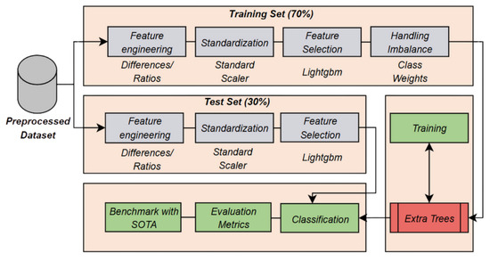
Figure 1. Proposed framework architecture.

2.1. Power-System Architecture and Dataset

The study employs a benchmark power system with two generators (G1, G2), four circuit breakers (BR1–BR4), three bus bars (B1–B3), and two high-voltage transmission lines, coordinated by four protective relays (R1–R4). A switch/router backbone links the relays, data acquisition, and supervisory control. The overall physical–cyber layout is summarized in Figure 2.

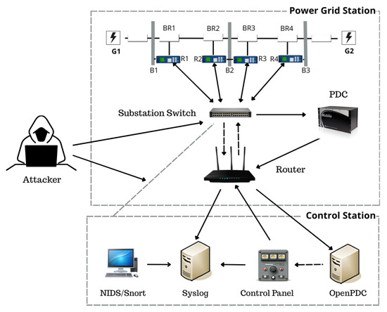
Figure 2. Architectural design of the MSU–ORNL power-grid system.

Distance protection on the relays issues trip commands to the breakers upon detected faults; in the absence of a validation layer, trips may also occur for spoofed or erroneous conditions. Operators can also issue manual trip instructions to the intelligent relays. In the cyber-attack scenarios, the adversary is assumed to have substation access and can inject false commands from the substation switch. A power distribution unit supplies loads, and system monitoring includes Snort, syslog, and a control panel.

The publicly available MSU–ORNL corpus of PMU-enabled power-grid events is employed, comprising three regimes: NoEvents, Natural, and Attack events. Each record aggregates synchronized phasor measurements from four PMUs together with a small set of OT/IT log indicators, so that both electrical behavior and control activity are observable in a common timeline.

Natural events include single-line-to-ground (SLG) faults at multiple locations along each line and routine line-maintenance operations. SLG faults exhibit characteristic voltage sags and current surges with distinctive sequence-component signatures; their spatial variation (e.g., 10–90% of line length) produces graded changes in phase angles and apparent impedance at the associated relays. Maintenance operations, by contrast, reflect deliberate de-energizing or relay disablement sequences, where logs indicate planned actions and PMU traces lack the abrupt precursors seen in genuine faults.

Attack events fall into three principal families that target protection logic and breaker actuation. Remote tripping command injection forces one or more breakers to open via malicious control messages, yielding relay/control-panel log activity without the preceding electrical precursors that normally justify a trip. Relay-setting change attacks alter distance-protection parameters so that valid faults do not trip (or trip late), extending fault currents and producing PMU–log inconsistencies; coordinated variants disable two relays simultaneously to widen impact. Data-injection (fault-replay) attacks manipulate measurement channels to mimic the phasor patterns of SLG faults at specified locations while pairing them with trip commands, thereby “explaining away” malicious openings as if they were protection-justified. Several scenarios combine these tactics (e.g., multi-relay command injection or setting changes during maintenance), increasing ambiguity between operational and adversarial causes. The specific PMU and log channels used in this study are summarized in Table 1.

Table 1. Different features of the dataset and their descriptions.

Feature	Description
PA1:VH–PA3:VH	Phase-to-neutral voltage angles
PM1:V–PM3:V	Phase-to-neutral voltage magnitudes
PA4:IH–PA6:IH	Line current angles
PM4:I–PM6:I	Line current magnitudes
PA7:VH–PA9:VH	Zero, positive, negative sequence voltage angles
PM7:V–PM9:V	Zero, positive, negative sequence voltage magnitudes
PA10:VH–PA12:VH	Zero, positive, negative sequence current angles
PM10:V–PM12:V	Zero, positive, negative sequence current magnitudes
F	System/relay frequency
DF	Rate of change in frequency ($df/dt$)
PA:Z	Relay apparent impedance magnitude
PA:ZH	Apparent impedance angle
S	Relay/IED status flag

Although the scenario logic is realistic at the protection/IED layer, the released traces are cleaner than field telemetry. The PMU channels originate from a high-fidelity simulator rather than a live substation network; therefore, channel noise, GPS time-sync jitter, relay actuation latency distributions, packet loss, and network-induced jitter are not explicitly represented. The dataset is thus well suited for evaluating discrimination between event types and protection-logic misuse, but does not fully capture end-to-end communication stack artifacts or stochastic measurement degradations that arise in operational PMU deployments.

From a classification perspective, this mixture of genuine electrical disturbances, operator-initiated actions, and adversarial manipulations makes discrimination non-trivial: different scenarios can imprint similar phasor trajectories while diverging in control/log evidence, and conversely, purely log-driven trips may appear without corroborating electrical signatures. Class imbalance adds a further challenge, as attack scenarios are more numerous than natural and no-event cases in the released sets.

Fifteen three-class datasets are considered, each containing roughly five thousand labeled samples. Every sample provides 128 features: 116 PMU channels (four PMUs, 29 measurements each) plus 12 log indicators. Across the corpus, 37 scenario templates were defined (28 attack, 8 natural, and 1 no-event). The class distribution for all 15 datasets is reported in Table 2.

Table 2. Distribution of instances for 15 MSU–ORNL power-grid datasets.

Dataset	Instances	Attack	Natural	NoEvents
Dataset-1	4966	3866	927	173
Dataset-2	5069	3525	1222	322
Dataset-3	5415	3811	1250	354
Dataset-4	5202	3402	1397	403
Dataset-5	5161	3680	1211	270
Dataset-6	4967	3490	1287	190
Dataset-7	5236	3910	1118	208
Dataset-8	5315	3771	1188	356
Dataset-9	5340	3570	1292	478
Dataset-10	5569	3921	1322	326
Dataset-11	5251	3969	1137	145
Dataset-12	5224	3453	1387	384
Dataset-13	5271	4118	950	203
Dataset-14	5115	3792	1274	79
Dataset-15	5276	3415	1347	514

2.2. Feature Engineering

In this study, raw features are enriched with simple yet expressive relational features. Let $x\in {\mathbb{R}}^d$ denote the vector of original channels. For each ordered pair $(i,j)$ with $i\ne j$, a difference and a ratio are formed as follows:

$$\begin{array}{cc}\hfill {\Delta }_{ij}& =x_i-x_j,\hfill \end{array}$$

(1)

$$\begin{array}{cc}\hfill {\rho }_{ij}& =\left\{\begin{array}{cc}{\displaystyle \frac{x_i}{x_j}},\hfill & x_j\ne 0,\hfill \\ 0,\hfill & x_j=0.\hfill \end{array}\right.\hfill \end{array}$$

(2)

From a power-system perspective, the differences ${\Delta }_{ij}$ play a role analogous to differential protection: they act as discrete spatial gradients between measurement locations (e.g., between two relays or between two phases at the same relay). Internal faults such as SLG faults create localized voltage sags and current surges that are more pronounced at some PMUs than others, so $|{\Delta }_{ij}|$ becomes large when one channel is “close” to the disturbance and the other is not. In contrast, global phenomena such as slow load changes, frequency drift, or common-mode noise tend to affect all channels in a similar way, so the corresponding differences remain small.

$$x_i\approx x_j\Rightarrow \left|{\Delta }_{ij}\right|\approx 0.$$

(3)

By working with ${\Delta }_{ij}$ rather than the raw $x_i$, common-mode effects are suppressed and spatially localized deviations are emphasized, which are patterns that distinguish faults and some cyber-events from normal operation.

Ratios ${\rho }_{ij}$, in turn, provide scale-invariant features that encode proportional relationships between channels. Many physical relationships in power systems are expressed in terms of ratios rather than absolute magnitudes: for example, ratios between sequence components (e.g., $V_0/V_1$, $I_2/I_1$) and between currents or voltages at opposite ends of a line are constrained by network impedances and operating conditions. Under natural faults, these ratios change in a way that is still consistent with network physics. For instance, an SLG fault at a given location alters positive-, negative-, and zero-sequence voltages in a structured manner, so ratios such as

$${\rho }_{ij}={\displaystyle \frac{V_{\mathrm{seq},i}}{V_{\mathrm{seq},j}}}$$

(4)

remain within ranges predicted by sequence-component theory and line parameters.

Cyber-attacks, however, need not respect these constraints. In remote tripping command scenarios, breakers are opened without the electrical precursors that normally justify a trip: PMU magnitudes and angles remain close to pre-disturbance values, yet relay and control-panel logs show trip activity. This produces ratios and differences between PMU channels and log indicators that are atypical for a physical fault (large log change with minimal phasor change). In false data injection or fault-replay scenarios, the attacker manipulates a subset of measurement channels to mimic a fault pattern at a particular location, but may not—or cannot—adjust all correlated quantities consistently (e.g., all sequence components across all relays). As a result, some ratios ${\rho }_{ij}$ become either abnormally large/small or mutually inconsistent when compared across relays and phases.

The NoEvents regime provides a third reference point: in the absence of faults or attacks, steady-state operation with small perturbations yields both

$$|{\Delta }_{ij}| \approx 0\mathrm{and}{\rho }_{ij}\approx 1$$

(5)

for most cross-relay and cross-phase pairs (after accounting for nominal phase shifts and topology).

2.3. Feature Selection

Expanding $x\in {\mathbb{R}}^d$ into pairwise relations yields $d(d-1)$ differences and $d(d-1)$ ratios in addition to the d originals—an $O\left(d^2\right)$ space that is expressive but redundant. An embedded selector based on LightGBM is therefore adopted. LightGBM is a fast, distributed gradient-boosting framework built on decision-tree learners and widely used for regression, ranking, and classification [27]. As a boosting method, it fits many shallow trees sequentially: In each round, a new tree is fit to the negative gradients (residuals) of the loss at the current model, so harder samples (with larger residuals) naturally influence the next tree more. The final predictor is an additive sum of trees, each scaled by a step size ${\alpha }_q$ determined through loss minimization. It can be written as

$$f\left(x\right)={\displaystyle \sum _{q=1}^Q}{\alpha }_{q}T(x,{\theta }_q),$$

(6)

where $T(x,{\theta }_q)$ is the qth tree with parameters ${\theta }_q$ and ${\alpha }_q$ is its step size (weight). Training seeks the function f that minimizes the empirical risk over H samples,

$${\displaystyle \underset{f}{min}}{\displaystyle \sum _{h=1}^H}L\left(y_h,f\left(x_h\right)\right),$$

(7)

with $L(·,·)$ the chosen loss (e.g., logistic for classification). In each boosting round, a new tree is fit to improve this objective.

In this study, a LightGBM classifier (Table 3) is fit on the training set to quantify the importance of each engineered relation. The model employs gradient boosting decision trees (boosting_type=gbdt) with 100 estimators. Predictors are ranked using their cumulative split gain—the total reduction in loss contributed by each feature across all splits and trees. After evaluating multiple retention thresholds, keeping the top 300 features was found to provide the best balance between accuracy and model compactness. This configuration preserves nonlinear interactions, enables correlated relations to compete for informative splits, and yields a compact subset that retains the most discriminative pairwise structure for downstream classification.

Table 3. LightGBM hyperparameters.

Hyperparameter	Value
boosting_type	gbdt
n_estimators	100
learning_rate	0.10
num_leaves	31
max_depth	−1
min_child_samples	20
subsample	1.0
subsample_freq	0
colsample_bytree	1.0
reg_alpha	0.0
reg_lambda	0.0
random_state	42
n_jobs	−1

2.4. Class-Imbalance Handling

In the MSU–ORNL dataset (Table 4), the class imbalance is modest in the binary case (Attack vs. Natural) but substantially more pronounced in the three-class setting, where Attack dominates both Natural and NoEvents. Left unchecked, most learners minimize loss by favoring the majority class, which depresses recall on the scarce classes. Class weighting counters this by scaling each example’s contribution to the training objective according to its class frequency: mistakes on minority classes are penalized more, and mistakes on the majority are penalized less. Concretely, inverse-frequency weights are computed on the training fold and passed to Extra Trees during final fitting,

$$\begin{array}{c}\hfill w_c={\displaystyle \frac{N_{\mathrm{tr}}}{C{n}_{c,\mathrm{tr}}}},\end{array}$$

(8)

where $n_{c,\mathrm{tr}}$ is the number of training samples in class c, $N_{\mathrm{tr}}={\sum }_c{n}_{c,\mathrm{tr}}$, and C is the number of classes. Each sample in class c inherits $w_c$, and these weights directly influence impurity-based splits.

Table 4. Class imbalance over three-class and binary data.

	Class	Ratio	Samples		Class	Ratio	Samples
Three-class	Attack	0.7102	55,663	Binary	Attack	0.7102	55,663
	Natural	0.2336	18,309		Natural	0.2898	22,714
	NoEvents	0.0562	4405

In gradient-boosted trees this enters via per-example gradients/hessians; in randomized trees, class weights adjust the proportion of each class in a node when calculating impurity (e.g., Gini or entropy). Instead of using raw sample counts, the algorithm uses weighted proportions

$$\begin{array}{c}\hfill p_c^{\prime }={\displaystyle \frac{w_c·n_c}{{\sum }_{j=1}^C{w}_j·n_j}},\end{array}$$

(9)

where $n_c$ is the number of samples of class c in the node. The impurity criterion is then computed using these weighted proportions $p_c^{\prime }$. This ensures that splits are evaluated based on a rebalanced class distribution, where minority classes contribute more to the impurity calculation. As a result, the tree is more likely to select splits that better separate underrepresented classes, improving their recall without requiring explicit resampling.

This choice contrasts with resampling, which changes the composition of the training set by duplicating minority samples (oversampling), discarding majority samples (undersampling), or synthesizing new points (e.g., SMOTE variants). Resampling can be effective, but it also alters the empirical distribution seen during training and may introduce artifacts in high-dimensional relational spaces (e.g., ratio features). Class weighting leaves the sample set intact and instead rebalances the learning signal in the loss, so evaluation on validation/test sets reflects the original class proportions.

2.5. Proposed Model

In this study, Extremely Randomized Trees (Extra Trees) proposed by Geurts et al. [28] are adopted as the final classifier. Compared with Random Forests, Extra Trees (i) randomly select K features at each node and draw a random split threshold for each, then choose the best among these random candidates, and (ii) grow trees on the full dataset without bootstrap. This stronger node-level randomization improves diversity and reduces variance—beneficial for high-dimensional, correlated predictors from relational expansion [24]. Figure 3 shows the algorithm framework and Table 5 presents the hyperparameters used.

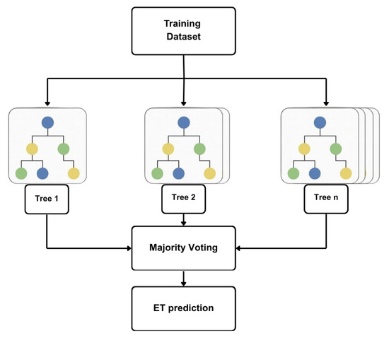
Figure 3. The framework of the Extra Trees algorithm.

Table 5. Extra Trees model configuration.

Hyperparameter	Value
Estimator	ExtraTreesClassifier
$n_{\mathrm{estimators}}$	600
max_features	$\sqrt{d}$
min_samples_leaf	2
max_depth	None
bootstrap	False
class_weight	balanced
random_state	42
n_jobs	$-1$

For classification, the ensemble prediction is the majority vote or averaged class probability across trees. For regression, the ensemble follows Breiman’s formulation [29],

$$\begin{array}{c}\hfill \widehat{f}\left(x\right)={\displaystyle \frac{1}{M}}{\displaystyle \sum _{m=1}^M}{h}_m\left(x\right)\end{array}$$

(10)

where $h_m\left(x\right)$ is the mth tree prediction and M the number of trees.

2.6. Evaluation Metrics

To better assess the effectiveness of the proposed framework, four standard measures—accuracy, precision, recall, and the F1-score are reported. Accuracy is the fraction of correctly classified samples; precision measures the share of predicted positives that are truly positive; recall measures the share of actual positives that are recovered; and F1 is the harmonic mean of precision and recall. Formally,

$$\begin{array}{c}\hfill \mathrm{Accuracy}={\displaystyle \frac{\mathrm{TP}+\mathrm{TN}}{\mathrm{TP}+\mathrm{TN}+\mathrm{FP}+\mathrm{FN}}}\end{array}$$

(11)

$$\begin{array}{c}\hfill \mathrm{Precision}={\displaystyle \frac{\mathrm{TP}}{\mathrm{TP}+\mathrm{FP}}}\end{array}$$

(12)

$$\begin{array}{c}\hfill \mathrm{Recall}={\displaystyle \frac{\mathrm{TP}}{\mathrm{TP}+\mathrm{FN}}}\end{array}$$

(13)

$$\begin{array}{c}\hfill \mathrm{F}1\text{-}\mathrm{Score}={\displaystyle \frac{2\mathrm{Precision}\times \mathrm{Recall}}{\mathrm{Precision}+\mathrm{Recall}}}\end{array}$$

(14)

where $\mathrm{TP}$, $\mathrm{TN}$, $\mathrm{FP}$, and $\mathrm{FN}$ denote true positives, true negatives, false positives, and false negatives, respectively. In the binary task, Attack is the positive class; in the three-class task, metrics are computed one-vs.-rest for each class and reported as macro-averages over Attack, Natural, and NoEvents.

3. Results and Discussion

3.1. Experimental Environment

The proposed model is implemented with Python 3.9.15 and JupyterLab 4.4.6 with scikit-learn 1.6.1, TensorFlow 2.19.1, NumPy 1.26.0, and Pandas 2.3.1 on Windows 10. The workstation has an AMD Ryzen 5 7600X CPU (12 logical cores), 32 GB RAM, and an NVIDIA GeForce RTX 3090 Ti (24 GB VRAM). The steps taken include data preprocessing, feature selection, data splitting, model development, and evaluation.

3.2. Model Evaluation

To comprehensively assess the predictive performance of the proposed pipeline on PMU–log data, the fifteen MSU–ORNL datasets serve as the evaluation benchmark. First, a stratified 70/30 train–test split is applied to each dataset. The full pipeline (feature engineering, standardization, LightGBM feature selection, and class-balanced Extra Trees) is fitted on the training portion and evaluated on the held-out test set. Results are shown in Table 6.

Table 6. Proposed method performance on selected features set (70–30 setup).

Dataset	Multiclass				Binary
	Acc	PR	RC	FS	Acc	PR	RC	FS
Dataset-1	0.9870	0.9892	0.9710	0.9800	0.9870	0.9856	0.9762	0.9808
Dataset-2	0.9858	0.9890	0.9781	0.9835	0.9851	0.9838	0.9805	0.9822
Dataset-3	0.9819	0.9825	0.9677	0.9749	0.9819	0.9817	0.9745	0.9780
Dataset-4	0.9742	0.9819	0.9644	0.9729	0.9902	0.9901	0.9882	0.9892
Dataset-5	0.9838	0.9829	0.9791	0.9808	0.9810	0.9821	0.9711	0.9764
Dataset-6	0.9767	0.9783	0.9697	0.9739	0.9818	0.9797	0.9761	0.9779
Dataset-7	0.9862	0.9896	0.9815	0.9855	0.9834	0.9841	0.9712	0.9774
Dataset-8	0.9870	0.9861	0.9825	0.9841	0.9857	0.9855	0.9791	0.9822
Dataset-9	0.9708	0.9730	0.9609	0.9668	0.9756	0.9738	0.9708	0.9723
Dataset-10	0.9882	0.9864	0.9837	0.9850	0.9908	0.9922	0.9857	0.9889
Dataset-11	0.9786	0.9821	0.9735	0.9777	0.9820	0.9760	0.9740	0.9750
Dataset-12	0.9756	0.9744	0.9658	0.9700	0.9825	0.9822	0.9789	0.9805
Dataset-13	0.9897	0.9854	0.9865	0.9859	0.9897	0.9899	0.9798	0.9847
Dataset-14	0.9886	0.9896	0.9896	0.9896	0.9851	0.9863	0.9747	0.9803
Dataset-15	0.9787	0.9836	0.9654	0.9742	0.9842	0.9846	0.9806	0.9826
Average	0.9822	0.9836	0.9746	0.9790	0.9844	0.9839	0.9774	0.9806
Std. dev.	0.0060	0.0052	0.0090	0.0067	0.0040	0.0050	0.0051	0.0047
95% CI low	0.9789	0.9807	0.9696	0.9753	0.9822	0.9811	0.9746	0.9780
95% CI high	0.9855	0.9865	0.9796	0.9827	0.9866	0.9866	0.9803	0.9832

Under this setup, the model maintains strong predictive performance across all datasets, achieving an average multiclass accuracy of 0.9822 and binary accuracy of 0.9844. The low standard deviations (not exceeding $0.009$ for any metric) and the narrow 95% confidence intervals (e.g., accuracy CI: $[0.9789,0.9855]$ for multiclass and $[0.9822,0.9866]$ for binary) confirm the statistical stability of the pipeline. The highest accuracies are recorded for Dataset-10, Dataset-13, and Dataset-14, each surpassing $0.988$, underscoring the method’s ability to adapt effectively across diverse operating conditions while maintaining consistent classification quality.

To assess bias under class imbalance, ROC–AUC is computed over test predictions from all 15 datasets combined as shown in Figure 4. The binary and multiclass curves both show near-perfect separability, indicating that the model maintains high discriminative capability even in the presence of imbalanced data.

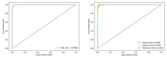
Figure 4. ROC curves for binary (left) and multiclass (right).

To further validate the robustness of the proposed approach and quantify performance variability under repeated resampling, stratified 10-fold cross-validation is applied to each dataset. This procedure generates ten independent train–test partitions per dataset, with the full pipeline re-fitted in each fold, allowing the model’s stability to be evaluated across multiple resampled splits rather than a single fixed division. The reported variability estimates are averaged across the fifteen datasets, and the detailed results are shown in Table 7.

Table 7. Proposed method performance on selected features set (10-fold cross-validation).

Dataset	Multiclass				Binary
	Acc	PR	RC	FS	Acc	PR	RC	FS
Dataset-1	0.9900	0.9899	0.9807	0.9857	0.9883	0.9869	0.9801	0.9827
Dataset-2	0.9821	0.9844	0.9773	0.9810	0.9825	0.9815	0.9760	0.9793
Dataset-3	0.9867	0.9884	0.9787	0.9845	0.9865	0.9850	0.9810	0.9836
Dataset-4	0.9870	0.9902	0.9866	0.9882	0.9860	0.9880	0.9823	0.9844
Dataset-5	0.9867	0.9890	0.9829	0.9860	0.9878	0.9871	0.9814	0.9849
Dataset-6	0.9834	0.9872	0.9789	0.9842	0.9862	0.9855	0.9806	0.9849
Dataset-7	0.9878	0.9913	0.9838	0.9872	0.9894	0.9911	0.9823	0.9859
Dataset-8	0.9855	0.9816	0.9790	0.9810	0.9881	0.9859	0.9819	0.9848
Dataset-9	0.9805	0.9807	0.9755	0.9780	0.9839	0.9812	0.9794	0.9817
Dataset-10	0.9851	0.9860	0.9809	0.9845	0.9860	0.9861	0.9812	0.9839
Dataset-11	0.9844	0.9890	0.9793	0.9837	0.9859	0.9855	0.9831	0.9804
Dataset-12	0.9864	0.9877	0.9802	0.9849	0.9866	0.9869	0.9849	0.9850
Dataset-13	0.9899	0.9872	0.9828	0.9849	0.9879	0.9880	0.9850	0.9865
Dataset-14	0.9876	0.9855	0.9861	0.9880	0.9866	0.9839	0.9819	0.9828
Dataset-15	0.9831	0.9820	0.9778	0.9806	0.9862	0.9860	0.9837	0.9848
Average	0.9857	0.9869	0.9810	0.9838	0.9865	0.9860	0.9806	0.9832
Std. dev.	0.0046	0.0064	0.0086	0.0064	0.0045	0.0051	0.0072	0.0056
95% CI Low	0.9829	0.9829	0.9756	0.9798	0.9838	0.9828	0.9762	0.9797
95% CI High	0.9886	0.9909	0.9863	0.9877	0.9893	0.9892	0.9851	0.9867

Under this setup, the model achieves an average multiclass accuracy of 0.9857 and binary accuracy of 0.9865, with precision, recall, and F1-scores following the same trend. The variability reported in Table 7 reflects the fold-wise standard deviation computed for each dataset and then averaged across all 15 datasets. The fold-wise dispersion remains small (multiclass: $0.0046$–$0.0086$; binary: $0.0045$–$0.0072$), corresponding to narrow 95% confidence intervals, which confirms the stability and statistical robustness of the proposed approach. High-performing datasets such as Dataset-1, Dataset-7, and Dataset-13 consistently achieve accuracies and F1-scores around or above 0.988, further demonstrating that the model maintains strong discriminative ability across repeated resampling.

Overall, the proposed pipeline performs consistently well across all fifteen datasets, maintaining high accuracy, precision, recall, and F1 in both evaluation regimes. The model remains stable despite the heterogeneous MSU–ORNL conditions, and the low standard deviations and narrow confidence intervals indicate that performance fluctuations are minimal.

Finally, computational efficiency is quantified. Across all 15 datasets, the average detection time during the 70/30 evaluation is 84.9 ms per test split for the binary task and 91.5 ms for the multiclass task, measured on standard CPU hardware. These sub-100 ms inference times indicate that, on the evaluated hardware and benchmark, the method is computationally lightweight and may be suitable for near real-time PMU-stream processing, while avoiding the GPU requirements and longer inference paths often associated with deep learning-based intrusion detection systems.

3.3. Comparison with Prior Works on the MSU–ORNL Dataset

To contextualize performance, the proposed scheme is contrasted with five recent lines of work on the MSU–ORNL benchmark: a metaheuristic feature selection–ensemble (Panthi and Das; BGWO-based) [22], a deep ensemble with metaheuristic optimization (Naeem et al.) [23], a graph-driven kernel attention network (Wu et al., GraphKAN) [24], an optimized Autoencoder–GRU ensemble with Grey Wolf-based feature selection (Dhinu Lal and Varadarajan) [26], and a statistical ExtraTrees–AdaBoost model with NCA-based feature extraction (Murugesan et al., SAML-Triple) [25]. Where individual dataset results are available, comparisons are made on a per-dataset basis, as shown in Table 8.

Table 8. Comparative accuracy per-dataset with prior works on binary and multiclass tasks.

Dataset	Panthi and Das [22]		Naeem et al. [23]		Wu et al. [24]		Proposed Model
	Binary	Multi	Binary	Multi	Binary	Multi	Binary	Multi
Dataset-1	97.20	98.07	–	98.10	97.82	98.99	98.70	98.70
Dataset-2	97.00	97.36	–	98.40	97.29	98.21	98.51	98.58
Dataset-3	97.30	98.41	–	99.00	98.45	98.62	98.19	98.19
Dataset-4	97.07	98.07	–	98.10	97.68	98.33	99.02	97.42
Dataset-5	98.07	98.33	–	98.00	98.07	98.92	98.10	98.38
Dataset-6	96.96	97.05	–	98.70	96.34	97.95	98.18	97.67
Dataset-7	97.71	98.12	–	98.60	98.95	98.27	98.34	98.62
Dataset-8	97.74	97.36	–	98.50	99.30	99.43	98.57	98.70
Dataset-9	95.79	97.45	–	97.60	92.83	97.78	97.56	97.08
Dataset-10	98.01	97.40	–	98.30	98.01	98.87	99.08	98.82
Dataset-11	97.60	97.23	–	97.80	99.27	99.31	98.20	97.86
Dataset-12	97.76	98.63	–	97.40	96.86	98.68	98.25	97.56
Dataset-13	97.80	97.74	–	98.70	98.40	99.13	98.97	98.97
Dataset-14	98.04	97.21	–	97.70	97.86	98.71	98.51	98.86
Dataset-15	98.14	98.03	–	98.30	97.38	97.26	98.42	97.87
Average	97.53	97.70	–	98.21	97.63	98.66	98.44	98.22

On the binary task, the proposed pipeline averages 98.44% accuracy, exceeding GraphKAN (97.63%) and the BGWO-based ensemble (97.53%) by 0.81 and 0.91 percentage points, respectively. Per-dataset analysis indicates the proposed model attains the highest accuracy on 10/15 datasets (D1, D2, D5–D6, D9–D10, D12–D15), with competitive performance on the remaining sets where GraphKAN occasionally performs better (e.g., D3, D4, D7, D8, D11).

On the ternary task, the method averages 98.22% accuracy, closely matching Naeem et al. (98.21%) and within 0.44 percentage points of GraphKAN (98.66%), while surpassing the BGWO-based ensemble (97.70%). Per-dataset analysis indicates the proposed model attains the highest multiclass accuracy on 3/15 datasets (D2, D7, D14), whereas GraphKAN is stronger on many others (e.g., D1, D3–D6, D8–D13), and Naeem et al. is competitive on D15.

To further extend the comparison to all five studies, Table 9 summarizes average binary and multiclass accuracies. Here, the proposed model surpasses all prior approaches on binary classification and remains within 0.4% of the best deep architecture (GraphKAN) on multiclass detection.

Table 9. Comparative average accuracy with prior works on binary and multiclass tasks.

Method	Binary Accuracy (%)	Multiclass Accuracy (%)
Panthi and Das [22] (BGWO)	97.53	97.70
Naeem et al. [23] (Deep Meta-Ensemble)	–	98.21
Wu et al. [24] (GraphKAN)	97.63	98.66
Dhinu Lal and Varadarajan [26] (Autoencoder–GRU)	-	95.82
Murugesan et al. [25] (SAML-Triple)	-	98.25
Proposed Model	98.44	98.22

Overall, the proposed approach is strongest on the binary task and attains the highest task-averaged score when weighting binary and ternary accuracies equally (98.33% vs. 98.15% for GraphKAN). Taken together, the evidence on the MSU–ORNL benchmark suggests that relation-centered features, followed by embedded selection and an Extra Trees backend, provide a competitive alternative to heavier deep architectures, particularly for high-fidelity binary intrusion detection, while remaining highly competitive in the ternary classification setting.

3.4. Comparison with Classical and Ensemble Baseline Models

To provide a comprehensive comparison, a representative suite of baselines was implemented: Random Forest (RF), XGBoost (XGB), Logistic Regression (LR), Decision Tree (DT), Bagging Classifier (BC), LightGBM (LGBM), K-nearest neighbors (KNN), and CatBoost (CB). These models span both ensemble methods (RF, XGB, BC, CB, LGBM) and classical baselines (DT, LR, KNN), offering complementary inductive biases for PMU/EMS data: bagged ensembles robust to noisy measurements and feature interactions (RF, BC), boosted trees tailored to complex tabular patterns (XGB, CB, LGBM), shallow or linear decision boundaries (DT, LR), and instance-based learning (KNN). All models shared the same preprocessing pipeline—pairwise ratios and differences, standardization, LightGBM-based feature selection, and a stratified $70/30$ split—with all baselines tuned under this unified protocol.

Across this unified pipeline, the proposed model consistently outperforms these baselines in accuracy and robustness. In the multiclass setting (Figure 5), the Extra Trees Classifier achieves the strongest overall accuracy and F1, maintaining the most stable precision–recall balance across datasets. This stability is notable given the variability in data distributions across operational scenarios. LGBM ranks second, with performance close to ETC, followed by XGB, RF, and CatBoost. BC and KNN remain competitive but moderately less stable, likely due to sensitivity to feature scaling and local data density. In contrast, DT and LR show larger drops in recall and F1, reflecting difficulty in separating closely related operating states and highlighting the limits of simpler models for PMU/EMS data. Across all 15 datasets, most models show low variability, with ETC reaching an accuracy standard deviation of 0.0064 compared to 0.0057 for LGBM and 0.0083 for XGB.

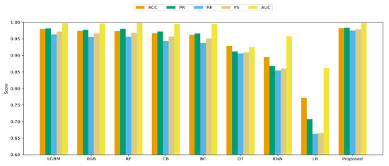
Figure 5. Multiclass results for baseline models and the proposed method.

On the binary task (Figure 6), the Extra Trees Classifier again delivers the highest performance across all metrics, confirming strong generalization and discrimination. It surpasses the strongest baselines (LGBM, RF, and XGB) in accuracy, precision, recall, and F1, with consistent gains across all metrics. LGBM, RF, and XGB remain highly competitive, whereas DT and LR show marked degradation in recall, yielding higher false negative counts. Most models also show low variability in the binary task, with ETC achieving an accuracy standard deviation of 0.0046 versus 0.0047 for LGBM and 0.0064 for XGB.

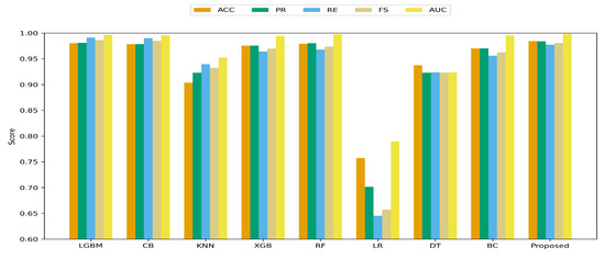
Figure 6. Binary results for baseline models and the proposed method.

In both multiclass and binary settings (Figure 7 and Figure 8), the Extra Trees Classifier exhibits the most diagonal confusion structures, confirming strong class separation and minimal misclassification. In the binary case ETC reaches only 232 FN/105 FP, with RF and LGBM similarly low (347/105 and 272/129) and XGB slightly higher (377/144), whereas LR and DT remain substantially weaker. The same pattern holds in the multiclass setting: ETC records only 241 Natural→Attack and 99 Attack→Natural errors, with RF and LGBM also compact (415/82 and 137/100), while XGB is moderately higher and LR reaches 3254 and 263 such errors. These counts confirm that ensemble models (ETC/LGBM/RF/XGB) reduce both false positives and false negatives by factors of roughly 3–15× compared to linear or shallow monolithic baselines.

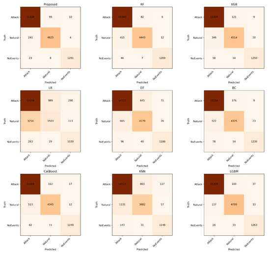
Figure 7. Multiclass confusion matrices for baselines and the proposed model.

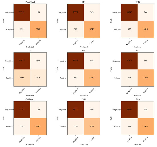
Figure 8. Binary confusion matrices for baselines and the proposed model.

3.5. Ablation Study

Given that the proposed framework leverages relation-driven feature engineering and embedded feature selection, an ablation study was conducted to systematically evaluate the contribution of each individual component. Each variant of the framework was tested by removing a single component while maintaining the rest of the pipeline unchanged, as detailed in Table 10. To validate the statistical significance of the observed performance differences, paired t-tests were applied across the 15 datasets. Effect sizes were quantified using Cohen’s d, ensuring that the differences reflect meaningful improvements rather than random variations.

Table 10. Ablation results averaged across 15 MSU–ORNL datasets.

Pipeline Variant	Multiclass		Binary
	Acc	AUC	Acc	AUC
Without FE and FS	96.83	99.49	97.10	99.46
Without FE	96.97	99.56	97.21	99.51
Without FS	97.40	99.73	97.80	99.73
Full Pipeline	98.22	99.87	98.44	99.84

FE = Feature Engineering, FS = Feature Selection.

On the binary task, the full configuration reaches 98.44% Accuracy and 99.84% AUC, outperforming FE-only (97.80%/99.73%), FS-only (97.21%/99.51%), and the configuration without FE and FS (97.10%/99.46%). Paired tests across datasets confirm that these differences are statistically reliable: Full vs. No FE and FS ($\Delta$Acc = +1.34 pp, $\Delta$AUC = +0.38 pp, $p<2\times {10}^{-8}$; $d\approx$ 3.0–3.5), Full vs. FE-only (+0.64 pp/+0.11 pp, $p\le 7\times {10}^{-6}$; $d\approx$ 1.8–2.0), and Full vs. FS-only (+1.23 pp/+0.33 pp, $p<2\times {10}^{-8}$; $d\approx$ 3.0). In practical terms, feature engineering provides most of the gain, while feature selection adds a smaller but statistically meaningful refinement, especially reflected in AUC.

For multiclass, the full pipeline reaches 98.22% Acc and 99.87% AUC, again outperforming FE-only (97.40%/99.73%), FS-only (96.97%/99.56%), and the configuration without FE and FS (96.83%/99.49%). These gaps are significant as well: Full vs. No FE and FS (+1.39 pp/+0.25 pp, $p\approx 4.5\times {10}^{-8}$; $d=$2.74–3.67), Full vs. FE-only (+0.81 pp/+0.09 pp, $p\approx {10}^{-5}$–${10}^{-6}$; $d=$1.61–2.12), and Full vs. FS-only (+1.25 pp/+0.23 pp, $p\approx {10}^{-8}$–${10}^{-9}$; d= 3.01–3.82). As in the binary case, relational feature engineering is the dominant driver of improvement, with feature selection providing statistically significant incremental gains.

The results clearly indicate that relation-based feature engineering is the most influential component of the pipeline. When this stage is omitted—either alone or together with selection—performance drops notably, underscoring how relational features drive separability between event classes.

3.6. Global Interpretation of Model Decisions Using SHAP

To enhance the interpretability of the model and provide insights into feature contributions, SHAP was used. SHAP values help elucidate how each feature impacts the model’s predictions, thereby offering a transparent view of the decision-making process. The SHAP summary plots in Figure 9, Figure 10 and Figure 11 visualize how individual features influence the model output for each class. Features are ordered by overall impact (y-axis), while each dot is a per-sample SHAP value (x-axis) colored by the corresponding feature value (blue = low, red = high), exposing both global importance and the directionality of effects, illustrated on Dataset 6.

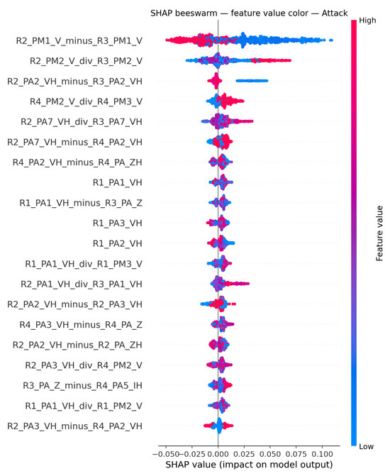
Figure 9. SHAP subplots for Attack class.

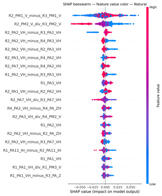
Figure 10. SHAP subplots for Natural class.

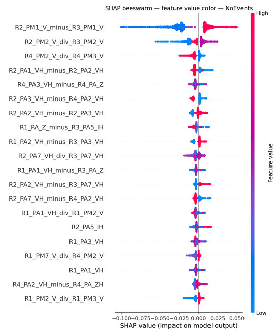
Figure 11. SHAP subplots for NoEvents class.

In Figure 9 (Attack), cross-relay voltage ratios and differences emerge as strong indicators, consistent with data-injection and remote-tripping scenarios that mimic fault signatures without physical precursors. For R2_PM1_V_minus_R3_PM1_V, large positive differences (red) cluster to the left, indicating pronounced voltage disparities between substations reduce the likelihood of an Attack prediction, whereas small or negative gaps push toward it. The ratio R2_PM2_V_div_R3_PM2_V is particularly decisive—ratios well above one lie to the right and strongly support Attack, while values near or below one oppose it. A similar directional pattern appears for the cross-relay angle gap R2_PA2_VH_minus_R3_PA2_VH, where lower or negative values nudge predictions toward Attack, and larger positive separations counteract it. By contrast, same-relay voltage ratios, such as R4_PM2_V_div_R4_PM3_V, exert little influence or act oppositely, indicating intra-relay discrepancies are less indicative of attack behavior.

In Figure 10 (Natural), cross-relay voltage ratios and cross-relay angle differences are the strongest indicators of faults, reflecting the phase imbalances that naturally arise during single-line-to-ground (SLG) faults and propagate across substations. Comparing voltage magnitudes across different relays is neither indicative of Natural nor opposed to it, as seen in R2_PM1_V_minus_R3_PM1_V. Low values of R2_PM2_V_div_R3_PM2_V align with Natural, whereas higher ratios push away. When the same phase is compared across relays, as in R2_PA2_VH_minus_R3_PA2_VH, larger gaps tend to slightly support Natural, suggesting mild phase deviations across substations are still consistent with natural events. Conversely, cross-relay differences involving different phases, such as R2_PA2_VH_minus_R4_PA3_VH and R2_PA3_VH_minus_R4_PA2_VH, exhibit opposite behaviors.

In Figure 11 (NoEvents), dense clouds near zero indicate that small inter-substation differences and ratios close to one typify normal operation. For R2_PM1_V_minus_R3_PM1_V, high values (red) form a thin rightward tail, so large positive cross-relay voltage differences push toward NoEvents, whereas small or negative gaps push away—precisely the opposite direction observed for Attack; this feature therefore separates Attack from NoEvents and is not informative for Faults. Likewise, R2_PM2_V_div_R3_PM2_V shows blue stretching left, indicating that low ratios drive the prediction away from NoEvents, while higher ratios support it; combined with the Natural figure (where low ratios are favored), this ratio cleanly separates NoEvents from Natural. Intra-relay angle and voltage contrasts (e.g., R2_PA1_VH_minus_R2_PA2_VH) stay close to zero and have little influence.

3.7. Local Interpretation of Model Decisions Using LIME

While SHAP provides global insights across the dataset, LIME complements it by explaining individual predictions. The LIME explanations in Figure 12 and Figure 13 use two-sided horizontal bars to show per-feature contributions for the predicted class: green bars on the right support the prediction; red bars on the left oppose it. Bar length encodes contribution magnitude.

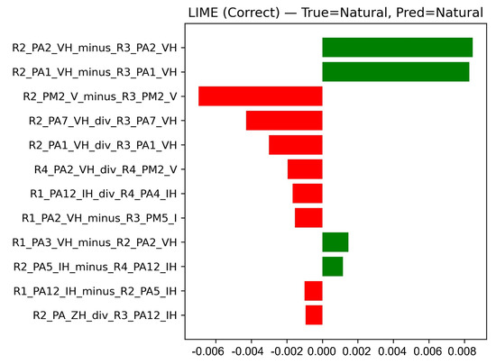
Figure 12. LIME local explanation—correct case.

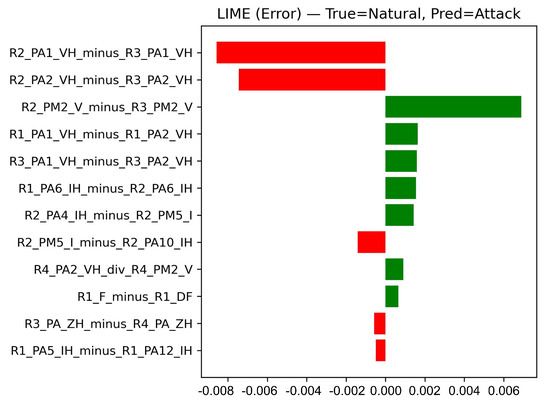
Figure 13. LIME local explanation—false alarm.

In Figure 12 (True = Natural, Pred = Natural), same voltage angle differences between different relays provide the strongest support for the prediction—most notably R2_PA2_VH_minus_R3_PA2_VH and R2_PA1_VH_minus_R3_PA1_VH. Opposing evidence includes same voltage magnitude differences such as R2_PM2_V_minus_R3_PM2_V, which SHAP confirmed do not contribute either toward or against the Natural class. Coherent same-voltage angle differences thus dominate, yielding a correct, high-confidence Natural prediction.

In Figure 13 (True = Natural, Pred = Attack), a strong supporting contribution from R2_PM2_V_minus_R3_PM2_V, together with several moderate positive features, favors the Natural class. However, R2_PA2_VH_minus_R3_PA2_VH and R2_PA1_VH_minus_R3_PA1_VH now push against predicting a natural event, contrary to what was seen with SHAP and observed in the correct prediction in Figure 12. The net effect is a false alarm caused by the limited separability between natural and attack for this specific case, particularly where data-injection attacks deliberately mimic the voltage and phase patterns of real faults.

4. Conclusions

This work introduced an ensemble framework for discriminating cyber-attacks, physical faults, and quiet operation in PMU-enabled smart grids. Relation-centered features were engineered using pairwise differences and ratios, embedded feature selection with LightGBM narrowed feature space, and a class-weighted Extra Trees classifier performed the final decision stage. Across 15 MSU–ORNL datasets, the pipeline achieved an average accuracy of 98.44% for the binary task and 98.22% for the multiclass task, with strong macro precision, recall, and F1-scores. Global and local explanations linked model decisions to the engineered features: cross-relay voltage ratios and differences provided the clearest indicators of Attack, while cross-relay voltage ratios and cross-relay angle differences characterized Natural events. The NoEvents class clustered around near-baseline differences and ratios close to one. These patterns are actionable for operators and confirm that simple relational signals, when paired with tree ensembles, can match or exceed heavier deep or graph-based models while offering superior interpretability and clearer separability between cyber attacks and faults. These conclusions reflect performance on the MSU–ORNL simulator-based benchmark. Future work will assess how the framework generalizes to additional grid configurations, field PMU telemetry, and environments with more realistic communication artifacts, and will also pursue finer-grained classification across specific cyber-attack scenarios and fault categories.

References

- Sullivan, J.E.; Kamensky, D. How cyber-attacks in Ukraine show the vulnerability of the U.S. power grid. Electr. J. 2017, 30, 30–35. [Google Scholar] [CrossRef]
- Jasiūnas, J.; Lund, P.D.; Mikkola, J. Energy system resilience—A review. Renew. Sustain. Energy Rev. 2021, 150, 111476. [Google Scholar] [CrossRef]
- Ashraf, S.; Shawon, M.H.; Khalid, H.M.; Muyeen, S.M. Denial-of-Service Attack on IEC 61850-Based Substation Automation System: A Crucial Cyber Threat towards Smart Substation Pathways. Sensors 2021, 21, 6415. [Google Scholar] [CrossRef]
- Liu, Y.; Ning, P.; Reiter, M.K. False data injection attacks against state estimation in electric power grids. In Proceedings of the 16th ACM Conference on Computer and Communications Security (CCS), Chicago, IL, USA, 9–13 November 2009; pp. 21–32. [Google Scholar] [CrossRef]
- Shereen, E.; Ramakrishna, R.; Dán, G. Detection and localization of PMU time synchronization attacks via graph signal processing. IEEE Trans. Smart Grid 2022, 13, 3627–3638. [Google Scholar] [CrossRef]
- Reeder, J.R.; Hall, T. Cybersecurity’s “Pearl Harbor” moment: Lessons from the Colonial Pipeline ransomware attack. Cyber Def. Rev. 2021, 6, 15–37. Available online: https://cyberdefensereview.army.mil/Portals/6/Documents/2021_summer_cdr/02_ReederHall_CDR_V6N3_2021.pdf (accessed on 30 September 2025).
- Tolba, A.; Al-Makhadmeh, Z. A cybersecurity user authentication approach for securing smart grid communications. Sustain. Energy Technol. Assess. 2021, 46, 101284. [Google Scholar] [CrossRef]
- Hamdi, N. A hybrid learning technique for intrusion detection system for smart grid. Sustain. Comput. Inform. Syst. 2025, 46, 101102. [Google Scholar] [CrossRef]
- Liu, W.; Ajay, P. Smart grid environment using blockchain-based key agreements. Meas. Sens. 2023, 26, 100992. [Google Scholar] [CrossRef]
- Mukherjee, D. A novel strategy for locational detection of false data injection attack. Sustain. Energy Grids Netw. 2022, 32, 100702. [Google Scholar] [CrossRef]
- Muneeswari, G.; Mabel Rose, R.A.; Balaganesh, S.; Jerald Prasath, G.; Chellam, S. Mitigation of attack detection via multi-stage cyber intelligence technique in smart grid. Meas. Sens. 2024, 25, 101077. [Google Scholar] [CrossRef]
- AlHaddad, U.; Basuhail, A.; Khemakhem, M.; Eassa, F.E.; Jambi, K. Ensemble Model Based on Hybrid Deep Learning for Intrusion Detection in Smart Grid Networks. Sensors 2023, 23, 7464. [Google Scholar] [CrossRef] [PubMed]
- Shrestha, R.; Mohammadi, M.; Sinaei, S.; Salcines, A.; Pampliega, D.; Clemente, R.; Sanz, A.L.; Nowroozi, E.; Lindgren, A. Anomaly detection based on LSTM and autoencoders using federated learning in smart electric grid. J. Parallel Distrib. Comput. 2024, 193, 104951. [Google Scholar] [CrossRef]
- Efatinasab, E.; Azadi, N.; Susto, G.A.; Ahmed, C.M.; Rampazzo, M. Fortifying smart grid stability: Defending against adversarial attacks and measurement anomalies. Sustain. Energy Grids Netw. 2025, 43, 101799. [Google Scholar] [CrossRef]
- Amin, B.M.R.; Hossain, M.J.; Anwar, A.; Zaman, S. Cyber Attacks and Faults Discrimination in Intelligent Electronic Device-Based Energy Management Systems. Electronics 2021, 10, 650. [Google Scholar] [CrossRef]
- Bitirgen, M.; Filik, T. A hybrid deep learning model for discrimination of physical disturbance and cyber-attack detection in smart grid. Int. J. Crit. Infrastruct. Prot. 2023, 40, 100582. [Google Scholar] [CrossRef]
- Liu, C.; Shi, Y.; Zhou, S.; Xu, L.; Li, Y. Distinguishable attack and fault detection in interconnected cyber–physical systems. Control Eng. Pract. 2025, 156, 106216. [Google Scholar] [CrossRef]
- Ramadan, M.; Abdollahi, F. A Hierarchical Approach for Isolating Sensor Faults from Un-Stealthy Attacks in Large-Scale Systems. J. Franklin Inst. 2024, 361, 106840. [Google Scholar] [CrossRef]
- Li, G.; Ren, L.; Pradhan, O.; O’Neill, Z.; Wen, J.; Yang, Z.; Fu, Y.; Chu, M.; Huang, J.; Wu, T.; et al. Emulation and Detection of Physical Faults and Cyber-Attacks on Building Energy Systems through Real-Time Hardware-in-the-Loop Experiments. Energy Build. 2024, 320, 114596. [Google Scholar] [CrossRef]
- Laythkhaleel, R.; Ibrahim, A.A.; Naseri, R.A.S.; Farhan, H.M. An Efficient Faults and Attacks Categorization Model in IoT-Based Cyber-Physical Systems Using Dilated CNN and BiLSTM with Multi-Scale Dense Attention Module. Biomed. Signal Process. Control 2024, 96(B), 106637. [Google Scholar] [CrossRef]
- Beaver, J.M.; Borges-Hink, R.C.; Buckner, M.A. An evaluation of machine learning methods to detect malicious SCADA communications. In Proceedings of the 2013 12th International Conference on Machine Learning and Applications (ICMLA), Miami, FL, USA, 4–7 December 2013; Volume 2, pp. 54–59. [Google Scholar] [CrossRef]
- Panthi, S.; Das, S. Intelligent intrusion detection scheme for smart power-grid using optimized ensemble learning on selected features. Int. J. Crit. Infrastruct. Prot. 2022, 39, 100567. [Google Scholar] [CrossRef]
- Naeem, H.; Ullah, F.; Srivastava, G. Classification of intrusion cyber-attacks in smart power grids using deep ensemble learning with metaheuristic-based optimization. Expert Syst. 2024, 42, e13556. [Google Scholar] [CrossRef]
- Wu, Y.; Zang, Z.; Zou, X.; Luo, W.; Bai, N.; Xiang, Y.; Li, W.; Dong, W. GraphKAN: A graph-driven intrusion detection framework for smart grids. Sci. Rep. 2025, 15, 8648. [Google Scholar] [CrossRef]
- Murugesan, N.; Velu, A.N.; Palaniappan, B.S.; Sukumar, B.; Hossain, M.J. Mitigating Missing Rate and Early Cyberattack Discrimination Using Optimal Statistical Approach with Machine Learning Techniques in a Smart Grid. Energies 2024, 17, 1965. [Google Scholar] [CrossRef]
- Dhinu Lal, M.; Varadarajan, R. Optimised Autoencoder-Based Ensemble Deep Learning Approaches for Cyber-Physical Event Classification Utilizing Synchrophasor PMU Data. Results Eng. 2025, 27, 105884. [Google Scholar] [CrossRef]
- Ke, G.; Meng, Q.; Finley, T.; Wang, T.; Chen, W.; Ma, W.; Ye, Q.; Liu, T.-Y. LightGBM: A highly efficient gradient boosting decision tree. Adv. Neural Inf. Process. Syst. (NeurIPS) 2017, 30, 3146–3154. Available online: https://proceedings.neurips.cc/paper_files/paper/2017/file/6449f44a102fde848669bdd9eb6b76fa-Paper.pdf (accessed on 20 August 2025).
- Geurts, P.; Ernst, D.; Wehenkel, L. Extremely randomized trees. Mach. Learn. 2006, 63, 3–42. [Google Scholar] [CrossRef]
- Breiman, L. Random forests. Mach. Learn. 2001, 45, 5–32. [Google Scholar] [CrossRef]
Disclaimer/Publisher’s Note: The statements, opinions and data contained in all publications are solely those of the individual author(s) and contributor(s) and not of MDPI and/or the editor(s). MDPI and/or the editor(s) disclaim responsibility for any injury to people or property resulting from any ideas, methods, instructions or products referred to in the content. |
© 2025 by the authors. Licensee MDPI, Basel, Switzerland. This article is an open access article distributed under the terms and conditions of the Creative Commons Attribution (CC BY) license (https://creativecommons.org/licenses/by/4.0/).