Efficiency of MPC Framework Cast to a Linear Programming Problem for a Servo Drive with Model Uncertainty

Abstract

Thepaper presents an efficient model predictive control framework formulated as a linear programming problem to control a servo drive with model uncertainty considerations from the viewpoint of the control performance. The model predictive framework is used to adopt $L_1$-type cost functions using absolute tracking errors, providing computational efficiency and enabling real-time implementation. A key contribution is the deployment of this approach on real hardware in a hardware-in-the-loop setting, supported by fully open-source code for Simulink Coder and C environments, verifying the solution scheme in real time. Experimental validation on a servo drive demonstrates the system’s tolerance for parameter uncertainties with slight performance degradation, resulting in an up to 18% increase in the considered control quality measure, between nominal parameters’ values and the worst configuration. The proposed linear programming approach enables constraint handling imposed on control signals and supports the arbitrary choice of prediction horizons and sampling intervals. The paper also includes a comprehensive derivation of the control law, controller implementation details, and stepwise experimental results showcasing the impact of uncertainties on control performance. This work and the attached code enable the authors to easily reproduce the proposed approach and extend it in their applications.

1. Introduction

Optimization-based techniques have made their way to exerting control tasks, both in the form of optimizing parameters of controllers, improving control performance, or using computational intelligence methods to pursue these tasks. Various control algorithms have been implemented, verified, and tuned using digital twins, on real hardware, or in hardware-in-the-loop contexts. Usually, a quadratic programming (QP) approach is used to obtain the optimal control solution, especially in model predictive control (MPC) contexts, as one of the most successful approaches.

Taking models into account requires consideration of model uncertainty, which might lead to tedious offline calculations related to classical or linear matrix inequality-based (LMI-based) robust control procedures, or incorporating these into the MPC framework [1,2,3,4] can be attempted to guarantee stability and performance under model uncertainties, as in [5]. However, these are computationally intensive, and the cited references do not handle the uncertainty issues, on the contrary to the solution proposed here.

Of course, the uncertainty of a model, not only its parameters but also its structural uncertainty, can be addressed through the MPC approach, usually leading to min–max optimization techniques which consider uncertainties expressed by unions of polytopes for a set of models considered. These approaches ensure not only robustness but also stability properties, despite model inaccuracies. Some MPC approaches take on worst-case scenarios [6] by solving a problem over uncertainty sets, which guarantees robust constraint satisfaction, but at the same time these are computationally heavy due to the nested optimization. The current paper’s linear programming (LP) formulation is a simpler alternative than handling uncertainty through explicit parameter grids and linear constraints.

The typical approaches are connected to algorithms that are impossible to use in time-demanding deployments, and as such, these could also be replaced by linear programming-based MPCs, offering efficient optimization with feasible global minimizers, enabling one to solve the problem with low computational burden, which is perfectly suitable for sampled-data control. As a counterexample, let us take the tube MPC, which generates a nominal trajectory and a robust invariant tube around it, containing all possible trajectories under uncertainty [7]. On the contrary, the current paper offers an online solution approach, emphasizing real-time efficiency, forming the step following our previous research [8].

Among the approaches that use partial parametrization and robust MPC, one has Youla parametrization, piece-wise affine approaches, and other robustifying approaches. The question, though, is if computational efficiency is taken into account, whether one should simply resort to simpler approaches and if they offer only slight performance degradation with those more advanced ones. With the abovementioned computational intelligence-based techniques, one can also incorporate machine learning characteristics to pre-identify a certain portion of information to diminish the impact of uncertainty on the overall performance in a rolling horizon optimization approach [9], or by using Deep Deterministic Policy Gradient reinforcement learning to reject uncertainties better [10].

The best answer as to why the LP approach is still considered an attractive solution is solely based on its computational efficiency, as well as its possibility of performing vast simulation campaigns, as in [8], to validate the effectiveness and robustness of the proposed control strategies, especially in Matlab–Simulink pairings in the context of hardware-in-the-loop procedures [11,12,13].

In the selected application, the rotational velocity control of a servo drive is exercised, and uncertainty is inherently interconnected even with such an application, not only from a parametric uncertainty perspective but also in time-varying disturbances [14]. One of these could be friction forces, which might affect the performance of high-precision servo systems [9] and lead to deterioration of the control quality under a predictive framework [15,16].

In the paper, the cost function under the MPC framework is replaced by sums of absolute errors instead of using sum-of-squares representation of the performance for the selected horizon [17]. This might be surprising, but the $L_1$ penalty function puts penalties proportional to absolute values of amplitudes of its arguments, on the contrary to $L_2$ representation, where “small” errors when squared produce a neglectful penalty. The same holds for the normalized control signal, which does not exceed a unity value. Initial research on this topic has been carried out in [8], in a fully simulated environment; thus, the current paper builds the new results upon the previous work of the authors.

Casting the model predictive control to an optimization problem has already been considered in [18]. The authors have obtained an explicit solution formulated on the basis of an $L_{\infty }$ norm, replaced eventually by an $L_1$ norm. Though a stability proof is given there, the procedure of obtaining the solution requires offline calculations using the affine piecewise systems technique to divide the state space into subregions, where appropriate actions need to take place. The identification of these regions along with the connected control laws uses multiparametric linear programming. Eventually, the authors decided to avoid direct calculations of the LP problem solution, rather to obtain the set of control policies in critical regions, connected to various sets of active constraints. The procedure should be approached with caution as the polyhedra related to the same linear gains need to be connected only when a convex set is obtained. However, the following question arises: what happens when the system description is uncertain and the corresponding polyhedral partitioning of the state space is inaccurate. In the current paper, we directly investigate the impact of parametric uncertainty from the viewpoint of performance, test the approach on the hardware, and present three performance indices related to various quality measures.

Another approach to reformulating the MPC problem can be found in [19], where the authors make an interesting attempt to connect hybrid modelling and the predictive control framework using a random forest approach. The main point is using the random forest method as the optimization solver. The reduction in the objective function is tackled using a random forest approach, and the overall problem is formulated as a mixed-integer linear program (or rather a set of problems). Obviously, powerful mixed-integer linear problem-solvers are available, but their use is limited by time constraints.

The novelty of the current paper is based on the deployment of an LP approach to obtain a real-time control system, with an MPC-based solution with the analysis of uncertainties taken into account and verified by means of experiments. It is not only prediction horizons which are taken as the starting point for the analysis but also uncertainties of the model’s parameters. What is more, as the main contribution, the paper also enables researchers to easily reproduce the results of the optimization routine and extend and add new features, as per full code of all the procedures given, to be used both under Simulink in hardware-in-the-loop experiments and also in C for alternative approaches, such as ROS nodes. As a Supplementary Material, all the necessary files are shared.

The key contributions of this paper are summarized as follows:

• Uncertainty vs. performance interplay analysis in various scenarios;
• Three types of performance indices considered;
• Availability of the open code for reproduction of further results;
• Hardware verification of the proposed methodology.

The question is why publish an open-source solution and describe the framework to use LPs to deploy model predictive control? The basic answer is to fully streamline the generation for open-source code, which can be directly deployed directly to a wide range of embedded control systems, which is a contribution of this paper. It is to be stated that recent papers have identified the following obstacles, which hinder the widespread adoption of MPC. These are challenges associated with deploying complex controllers on physical systems, as well as the scarcity of rapid prototyping tools for advanced methods, along with a limited reproducibility and reusability of model predictive controllers, which we fully align with [20]. The authors align to FAIR principles (findable, accessible, interoperable, reusable) for scientific data management and research software, and this is followed in this paper. At this cost, the theoretical contribution of this paper is limited, but the availability of the code is the added value. A similar approach can be found, e.g., in [21], where the authors use a much more demanding solver to obtain the optimal control, as in the case of the Newton method in [22]. The approach from the side of a linear program is definitely more appealing.

The structure of this paper is as follows: In Section 2, a short description of the adopted control strategy is given, along with information about the experimental setup. Section 3 provides information about the cost functions/performance indices considered in the paper. Section 4 presents the reformulation of the basic optimization task to the linear programming format, along with sample derivations. The controller implementation is given in Section 5, and Section 6 presents the results, in a step-by-step fashion, ending on the core of the paper, in the form of the results for the uncertain model. Finally, the last Section provides the discussion and outlines further research directions. The Appendix A, Appendix B, Appendix C, Appendix D and Appendix E which follow the paper present the code with appropriate comments, flowcharts of the algorithm, and a discussion of the sample stability proposition for the considered model.

2. Referred Control Strategy and Hardware

The predictive control task considered in the paper is mainly concerned with minimizing the performance index expressed by the absolute values of the error signal, and the implemented control signal,

$$\begin{array}{c}\hfill J(N_y,N_u)=\sum _{i=1}^{N_y}|r_{t+i}-{\widehat{y}}_{t+i}|+\sum _{i=1}^{N_u}{q}_u\left|u_{t+i-1}\right|,\end{array}$$

(1)

where $N_u$ and $N_y$ are prediction horizons of the input and output signals, respectively, and $q_u\ge 0$ is the weight put on the control signal component.

The reference $r_t$ is $N_y$ steps in advance, and ${\widehat{y}}_t$ is the prediction of the output signal usually calculated on the basis of the iterative equations, related to the linear model identified in the previous paper of the authors [8,23]. The absolute values result from casting the optimization task here to a linear program.

This performance index will eventually give rise to possible solutions of three types of predictive control-related optimization tasks, where $r_{t+i}-{\widehat{y}}_{t+i}$ is replaced by the error $e_{t+i}$ calculated on the basis of a state-space description in a tracking task, and the optimized control signals $u_{t+i-1}$ are obtained as the elements of the optimal decision variables vector, i.e., the optimal control vector subject to imposed constraints. For this reason, the explicit equations defining the prediction of the output signal are not necessary here and just serve the purpose of mirroring the traditional view of the performance index as the link to the classical MPC framework.

The concept of the control is presented in Figure 1, where decision variables define control actions in the horizon of $N_u$ samples and the evaluation of the tracking/regulation performance in $N_y$ samples. Since $N_y\ge N_u$, whenever $N_y-N_u>0$, the $N_y-N_u$ last samples of the control signal in the horizon $N_y$ are kept constant with the value taken from the $N_u$-th sample.

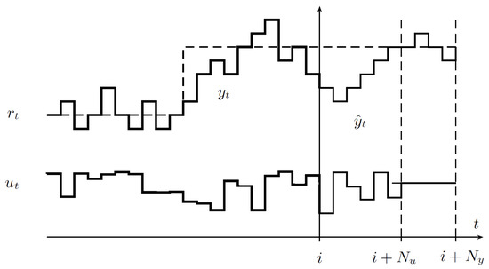
Figure 1. The concept of predictive control.

The information connected to the predicted output is calculated on the basis of the assumed model of the plant (here in the considered MPC with absolute values under the cost criterion, and it has a form of a linear input–output equation), possibly also taking uncertain knowledge concerning the model parameters into account.

The following controlled-ARMA model is considered

$$\begin{array}{c}\hfill A\left(q^{-1}\right)y_t=B\left(q^{-1}\right)u_{t-d},\end{array}$$

(2)

where $d>0$ is the the delay in the control channel value, and $A\left(q^{-1}\right)$ and $B\left(q^{-1}\right)$ are polynomials to be presented in the further part of the paper describing the linear model of the servo system.

At all times, the control signal $u_t$ is calculated on the basis of the optimization routine, where it is assumed that the error samples are known in horizon up to $N_y$, and as per the LP solved, it is constrained either in amplitude or amplitude and rate fashion.

The discrete time linearized model of the servo system with $u_t$ as its voltage input and $y_t$ as the rotational velocity can be put into a simple form

$${\displaystyle \frac{B\left(z^{-1}\right)z^{-d}}{A\left(z^{-1}\right)}}={\displaystyle \frac{b{z}^{-1}}{1-a{z}^{-1}}}$$

(3)

or alternatively in the state-space form

$$x_{t+1}=A{x}_t+b{u}_t.$$

(4)

The $(A,b)$ pair results from discretization of a continuous-time model of the servo drive (first-order inertia type, single-input, single-output system):

$$\begin{array}{ccc}\hfill A& =& {exp}^{-{\displaystyle \frac{T_s}{T}}},\hfill \\ \hfill b& =& k(1-A),\hfill \end{array}$$

where k and T denote gain and time constants of the continuous-time model, respectively, and $T_s$ denotes the sampling interval. The real values of the continuous-time model are $k=225\mathrm{rad}/\sec /\mathrm{V}$ and $T=1\sec$ and have been identified in [8].

The experimental setup of Inteco MSS is shown in Figure 2, and the parameters of the linear model of the servo system are cited after [23] and outlined in Table 1.

Figure 2. The modular servo system (MSS) of Inteco.

Table 1. Selected parameters of the Inteco MSS components.

Component	Parameters
DC motor	Buehler Motor GmbH, 1.12.044.236 model
	voltage 12 V, power 77 W,
	torque 250 mNm, maximum rotational velocity 3000 rpm, rated current 4.7 A
Load	Brass cylinder, weight 2.03 kg,
	diameter 66 mm, length 68 mm

The modular servo system has a nonlinear static characteristics which has been compensated by using a look-up table with the data related to the measurements to build its inverse. In addition, the potentiometer allowing for manual gain change in the power module visible as a yellow box in Figure 2 enables one to fix the amplification ratio of the tachogenerator manually, which resulted in performing all the experiments for the same gain of the linearized model without any drift from its nominal parameters [23]. During the experiments, all the reference velocities were chosen in such a way as to fully show the dynamics of the closed-loop system, avoiding overlong saturation of the normalized control input, resulting in an agile velocity change in the considered range of its values. The sampling interval $T_s$, to ensure proper balance between the need to recalculate control inputs, and the dynamics of the servo system, has been chosen as roughly 10% of the dominating time constant T of the linear model of the system.

The major challenge involved with the deployment of this control strategy on the real hardware has been to keep the calculations simple and with low computational burden. Thus, the quadratic cost functions related to model predictive control [24] have been replaced by absolute values (1). Secondly, the absolute values have been replaced by pairs of linear constraints imposed on the arguments of the absolute values, which enabled the authors to not only cast the problem to a linear programming one but also consider a number of performance indices presented in Section 3, while keeping the solution of the constrained linear programming problem simple to obtain a proper adaptation of MOSEK routines.

After initial trial-and-error attempts, MOSEK was the selected solver, as it allowed for the operation to be performed in a real-time regime on Inteco MSS, offered a reliable solution procedure, and used the controller code written in C to streamline the compilation by the Simulink Coder to the final code.

3. Considered Performance Measures and Experimental Setup

In order to conduct various experiments, the following performance indices have been taken into account:

• $J_1={\sum }_{i=1}^{N_y}\left|e_i\right|$;
• $J_2={\sum }_{i=1}^{N_y}\left|e_i\right|w_i$, with weights $w_i$ changing across the samples;
• $J_3={\sum }_{i=1}^{N_y}|e_i|+{\sum }_{i=1}^{N_u}{q}_u\left|u_i\right|$, with weight q for the control component.

In the case of the first performance index, with $e_i=r_i-y_i=r_i-(A{x}_{t+i-1}+b{u}_i)$, the problem ($\underline{u}={[u_1,u_2,\dots ,u_{N_u}]}^T$)

$$\underset{\underline{u}}{min}\sum _{i=1}^{N_y}\left|e_i\right|,$$

(5)

is brought to its linear form by the use of the dummy variable $\underline{t}={[t_1,t_2,\dots ,t_{N_y}]}^T$, with 

$$\begin{array}{ccc}\hfill \underset{\underline{u},\underline{t}}{min}& {\sum }_{i=1}^{N_y}{t}_i& \end{array}$$

(6)

$$\begin{array}{ccc}\hfill \mathit{s}.\mathit{t}.& -t_i\le e_i\le t_i& (i=1,\cdots ,N_y),\hfill \end{array}$$

(7)

$$\begin{array}{cc}& \underline{t}\ge \underline{0},\end{array}$$

(8)

where $N_y$ is an integer number of sampling intervals to give the observation horizon.

In the case of the second performance index, consecutive errors are taken with appropriate weights, increasing either linearly or exponentially. In the linear case,

$$w_i=a_{i}i,$$

(9)

where the i–th step falls within the considered horizon, and the directional coefficient is subject to change, e.g., as $a_i=(1+(i-1)0.1)$. In the case of exponentially changed weights,

$$w_i=i^{a_i}.$$

(10)

The final optimization problem becomes

$$\begin{array}{ccc}\hfill \underset{\underline{u},\underline{t}}{min}& {\sum }_{i=1}^{N_y}{t}_i{w}_i& \end{array}$$

(11)

$$\begin{array}{ccc}\hfill \mathit{s}.\mathit{t}.& -t_i\le e_i\le t_i& (i=1,\cdots ,N_y),\hfill \end{array}$$

(12)

$$\begin{array}{cc}& \underline{t}\ge \underline{0}.\end{array}$$

(13)

In the case of the last performance index, the optimization problem is formulated as

$$\underset{e_i,u_i}{min}\sum _{i=1}^{N_y}|e_i|+\sum _{i=1}^{N_u}{q}_u\left|u_i\right|.$$

(14)

Now, introducing dummy variables $\underline{t}={[t_1,t_2,\dots ,t_{N_y}]}^T$ and $\underline{k}={[k_1,k_2,\dots ,k_{N_u}]}^T$, one gets

$$\begin{array}{ccc}\hfill \underset{\underline{u},\underline{t},\underline{k}}{min}& {\sum }_{i=1}^{N_y}{t}_i+{\sum }_{i=1}^{N_u}{q}_u{k}_i.& \end{array}$$

(15)

$$\begin{array}{ccc}\hfill \mathit{s}.\mathit{t}.& -t_i\le e_i\le t_i& (i=1,\cdots ,N_y),\hfill \end{array}$$

(16)

$$\begin{array}{ccc}& -k_i\le u_i\le k_i& (i=1,\cdots ,N_u),\hfill \end{array}$$

(17)

$$\begin{array}{ccc}& \underline{t}\ge \underline{0},& \end{array}$$

(18)

$$\begin{array}{cc}& \underline{k}\ge \underline{0}.\end{array}$$

(19)

When the LP programs are solved, one could consider typical constraints easily, such as the symmetrical amplitude constraint with $\alpha \ge 0$ as the cut-off level

$$-\alpha \le u_i\le \alpha ,$$

(20)

or rate constraint with admissible rate $\beta \ge 0$

$$\beta \le u_i-u_{i-1}\le \beta .$$

(21)

4. Sample Derivation of the Control Law

Since the considered cost functions require the prediction of the output in $N_y$ horizon, and the following equation governs the model of the servo system (where A and b are the parameters resulting from the input–output equation, eventually replaced by their estimates),

$$x_{i+1}=A{x}_i+b{u}_i.$$

(22)

Thus, for every sampling interval, $T_s$ the future states can be given as

$$\begin{array}{ccc}\hfill x_i& =& A^i{x}_0+\sum _{j=0}^{i-1}{A}^{i-j-1}b{u}_j=\hfill \\ & =& A^i{x}_0+A^{i-1}b{u}_0+A^{i-2}b{u}_1+\cdots +Ab{u}_{i-2}+b{u}_{i-1},\hfill \end{array}$$

(23)

or in the other form

$$\begin{array}{ccc}\hfill x_i& =& \Phi x_0+{\underline{\Gamma }}^T\underline{U},,\hfill \end{array}$$

(24)

$$\begin{array}{ccc}\hfill e_i& =& r_i-x_i,\hfill \end{array}$$

(25)

with

• $\Phi =A^i$;
• ${\underline{\Gamma }}^T=\left[A^{i-1},A^{i-2},\cdots ,A^1,A^0\right]b$;
• $\underline{U}={\left[u_0,u_1,\cdots ,u_{i-2},u_{i-1}\right]}^T.$

Now, let $J_3$ be considered with $N_y=3$, $N_u=3$, $\alpha =0.8$, $\beta =0.3$, $q_u=30$, along with the assumption that the future reference signal samples and the current state measurement $x_0$ in the receding horizon are known at all times, which leads to

$$\begin{array}{cc}\hfill \underset{\underline{u},\underline{t},\underline{k}}{min}& {\sum }_{i=1}^{N_y}{t}_i+{\sum }_{i=1}^{N_u}30k_i\\ \hfill \mathit{s}.\mathit{t}.& {\forall }_{i\in \{1,2,3\}}-t_i\le e_i\le t_i,\\ & {\forall }_{i\in \{1,2,3\}}-k_i\le u_i\le k_i,\\ & {\forall }_{i\in \{1,2,3\}}-0.8\le u_i\le 0.8,\\ & {\forall }_{i\in \{1,2,3\}}-0.3\le u_{i-1}-u_i\le 0.3,\\ & \underline{t}\ge 0,\\ & \underline{k}\ge 0.\end{array}$$

(26)

In the above expression, variables $t_i$ replace border absolute values of the future tracking errors; thus, when $t_i\ge 0$ is minimized, it actually minimizes the $|e_{t+i}|$ value denoted here for the sake of brevity as the sequence $e_1$, $e_2$, …. The same holds in the case of $k_i\ge 0$ replacing $|u_{t+i-1}|$, referred to here as the $u_1$, $u_2$, …sequence.

The optimization task becomes

$$\begin{array}{cc}\hfill \underset{\underline{u},\underline{t},\underline{k}}{min}& {\sum }_{i=1}^3(t_i+30k_i)\\ \hfill \mathit{s}.\mathit{t}.& -t_1\le r_1-A{x}_0-b{u}_1\le t_1,\\ & -t_2\le r_2-A^2{x}_0-Ab{u}_1-b{u}_2\le t_2,\\ & -t_3\le r_3-A^3{x}_0-A^{2}b{u}_1-Ab{u}_2-b{u}_3\le t_3,\\ & {\forall }_{i\in \{1,2,3\}}-k_i\le u_i\le k_i,\\ & {\forall }_{i\in \{1,2,3\}}-0.8\le u_i\le 0.8,\\ & {\forall }_{i\in \{1,2,3\}}-0.3\le u_{i-1}-u_i\le 0.3,\\ & \underline{t}\ge 0,\\ & \underline{k}\ge 0.\end{array}$$

(27)

Moving the decision variables to the LHS, and the constants to the RHS

$$\begin{array}{cc}\hfill \underset{\underline{u},\underline{t},\underline{k}}{min}& t_1+t_2+t_3+30k_1+30k_2+30k_3\\ \hfill \mathit{s}.\mathit{t}.& -t_1\pm b{u}_1\le \pm r_1\mp A{x}_0,\\ & -t_2\pm Ab{u}_1\pm b{u}_2\le \pm r_2\mp A^2{x}_0,\\ & -t_3\pm A^{2}b{u}_1\pm Ab{u}_2\pm b{u}_3\le \pm r_3\mp A^3{x}_0,\\ & {\forall }_{i\in \{1,2,3\}}-k_i\pm u_i\le 0,\\ & {\forall }_{i\in \{0,1,2\}}\pm u_i\le 0.8,\\ & {\forall }_{i\in \{1,2,3\}}\pm u_i\le 0.3\pm u_{i-1},\\ & \underline{t}\ge 0,\\ & \underline{k}\ge 0.\end{array}$$

(28)

Whenever $N_u<N_y$, the last $N_y-N_u$ actions do not change the one calculated for $N_u$ step. This reformulation of a classical MPC problem enables one to use efficient LP solvers in real time, taking constraints into consideration, and it allows for a similar formulation for the remaining two performance indices.

5. Controller Implementation Issues Under LP Framework

In order to deploy the LP task on the hardware, specific C code was written, as a C-MEX S-function, and compiled as .mex64, Matlab Executable, and finally used in Simulink to perform hardware-in-the-loop experiments. The template used is presented in Appendix A.

The implementation of an LP problem under MOSEK [25], along with the comments, takes the form given in Appendix B.

The complete controller code is placed within mdlOutputs routine in the S-function. For the considered sample optimization problem

$$\begin{array}{ccc}\hfill \underset{\underline{x}}{max}& 3x_1+x_2+5x_3+x_4& \\ \hfill \mathit{s}.\mathit{t}.& 3x_1+x_2+2x_3& =30,\hfill \\ & 2x_1+x_2+3x_3+x_4& \ge 15,\hfill \\ & 2x_2+3x_4& \le 25,\hfill \\ & 0\le x_1\le \infty & ,\hfill \\ & 0\le x_2\le 10& ,\hfill \\ & 0\le x_3\le \infty & ,\hfill \\ & 0\le x_4\le \infty & ,\hfill \end{array}$$

it takes the form presented in Appendix B again. Obviously, the controller code for MPC is much more complicated, as it has, e.g., 33 constraints binding states, 88 constraints binding controls, and 250 non-zero entries in A. In order to streamline the comparison of the platforms for the readers of this paper, the authors have attached the C-code of the LP MOSEK routine, along with the .slx file, as a Supplementary Material.

Once the MPC is casted to an LP program, the final routine becomes the part of handling the S-function (mdlOutputs).

The remaining code includes solver-specific functions with the end of the loop when complete A matrix is created. Finally, the optimal value is calculated by calling MOSEK.

The reason for selecting the linear programming framework is that MOSEK is recognized for providing solvers with great performance both for linear and quadratic problems, though quadratic problems are more computationally demanding. Based on the benchmarks, e.g., [26], the solution time for QP under MOSEK is longer than for LP, potentially several times the computational cost depending on problem size and structure.

Despite the use of interior-point methods, the linear problems are naturally simpler, up to twice in comparison with the baseline time. LP solvers under MOSEK use interior-point or barrier methods, whereas in the case of QP problems, interior-point or active-set methods.

To reduce the computational burden, when there is no reason to take constraints into account while providing the optimal solution, the explicit solution of the predictive control problem using quadratic terms is used, as in [27], and to saturate the control signal at the specified level afterwards. This obviously does not take advantage over solving the exact constrained QP problem, but it does avoid potential bottlenecks when the sampling interval should be kept short.

6. Results

The presented experimental results have been carried out in a grid of $11\times 11$ configuration points, and averaged between 10 experiments each. The overall number of experiments in a grid was thus 10 times and 121 experiments.

To follow a step-by-step procedure, and to test the impact of the uncertainty of the parameters of the servo drive model, a series of experimental runs has been carried out to identify the configuration of the final experiment. At first, the impact of $N_y$ and $\alpha$ has been tested, with the amplitude cut-off constraint at the level

$$0.4\le \alpha \le 1,$$

(29)

and sampling intervals

• $T_s=0.05\sec (20\mathrm{per}\mathrm{time}\mathrm{constant}\mathrm{estimate});$
• $T_s=0.1\sec (10\mathrm{per}\mathrm{time}\mathrm{constant}\mathrm{estimate});$
• $T_s=0.2\sec (5\mathrm{per}\mathrm{time}\mathrm{constant}\mathrm{estimate})$

to test the impact of the cut-off level on the performance and raise the problem of sampling frequency.

In Figure 3, the performance index surface is presented, with three test points selected: blue (the worst case), green (medium case), and red (the best case). The parameter configurations for these points as a pair ($N_y$, $\alpha$) are given as (2, 0.47), (6, 0.70), (10, 0.95), respectively. It can be seen that even in the case of harder constraints, the increase in the prediction horizon $N_y$ can improve the behaviour of the system, which takes place especially in the case when the reference signal changes its value (bottom row).

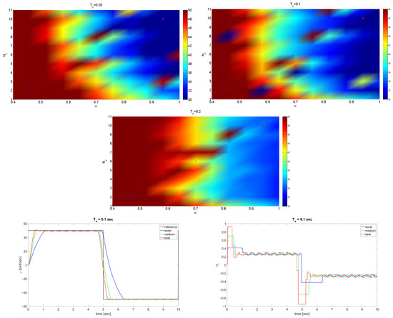
Figure 3. Surface of $J_1(N_y,\alpha )$ for three sampling intervals and the time plots.

Putting penalties on the future errors, as in the case of the $J_2$ index, resulted in the adverse result, as Figure 4 clearly presents the case that an increase in weights along time puts greater control attention to future errors, not to the nearest error samples, when there is no integral term in the open-loop system, leading to steady-state-like errors along the way.

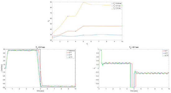
Figure 4. Plot of $J_2$ and corresponding time plots.

The final step of the experimental pre-study revolved around the impact of the control weights $q_u$ on the performance for different $(N_y,N_u)$ pairs, as shown in Figure 5. Again, as per no integral term action in the open-loop, the penalty on the control effort should be applied with caution (consult the bottom row), as severe penalties result in loss of tracking performance. Clearly, increasing prediction horizons results in better control performance, especially during the change in the reference signal.

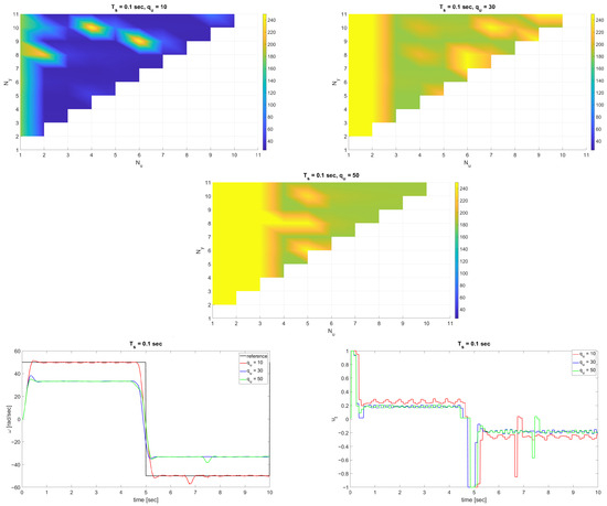
Figure 5. Surface of $J_3(N_u,N_y)$ for three $q_u$s and corresponding time plots.

The core of this paper is the analysis of the impact of the parametric uncertainty on the performance of the closed-loop system under the MPC framework, and to present broad experimental results. In order to conduct the experiments, parameters $(A,b)$ in (24) have been replaced with $(\widehat{A},\widehat{b})$ being functions of

$$\begin{array}{ccc}\hfill \widehat{k}& =& k{\delta }_k,\hfill \\ \hfill \widehat{T}& =& T{\delta }_T,\hfill \end{array}$$

with ${\delta }_k$ and ${\delta }_T$ introduced to mimic the uncertainty. All the experiments have been conducted with the intermediate sampling interval, $T_s=0.1\sec$ and $q_u=10$ with the following uncertainty ranges:

$$\begin{array}{ccc}\hfill 0.5\le & {\delta }_k& \le 1.5,\hfill \\ \hfill 0.5\le & {\delta }_T& \le 1.5.\hfill \end{array}$$

The reference profile has been taken as in the prior experiments, and the performance has been evaluated on the basis of the standard continuous-time IAE index calculated over the experiment horizon of 10 sec.

Since a vast experimental campaign has been conducted on the servo system, it has been observed that the nominal parameters, k and T, have a slight drift, resulting from the mechanical wear of the parts, gripping of the clutches holding the elements on the rail, replaced when needed, changes in the amplification ratio in the power stabilizer box, but most predominantly, the temperature of the components. The change in the gain as a thermal flow of the parameter has given the border values between 168 and 250, which had to be manually altered via the amplification potentiometer of the tachogenerator, so that eventually 225 was kept at all times.

Figure 6 presents a sample drift in parameters estimated by fitting the step response of a linear first-order model of the servo system to the step response of the Inteco MSS, and taking least-squares measure in the residuals of the fitting between the measured data, and the step response of the MSS model. Eventually, the rough estimate of the mean time constant across the experiments in an almost 30-min horizon was 100 experiments conducted one after another, which gave $\widehat{T}\approx 1\sec$, and $\widehat{k}\approx 225$, as considered in the paper.

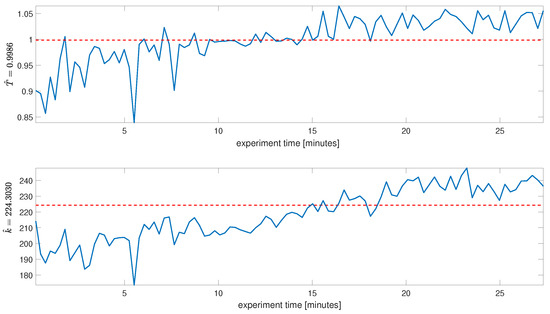
Figure 6. Experimental verification of the drift in nominal parameters of the fitted first-order inertia linear model.

In all the experiments conducted in this paper, the amplification ratio in the power box has been periodically verified to result in the gain of the best fitted model as 225.

Since the change in the time constant is 20% at maximum, and the change in the gain is almost the same, the authors have decided to introduce the uncertainties $({\delta }_k,{\delta }_T)$ in an even greater range to verify the performance degradation on the real hardware. Potential support for the uncertainty range in the time constant could be the variation in the moment of inertia of a servo system, when the load on the shaft changes, over a broad range of values.

Figure 7 presents the surfaces of IAE performance indices (left column) along with their zoomed-in versions (right column). In the bottom row, time plots for three selected configurations of uncertainties are given as a pair (${\delta }_k$, ${\delta }_T$) as (0.6, 0.6), (1, 1), and (1.4, 1.4), respectively (worst, best, and medium).

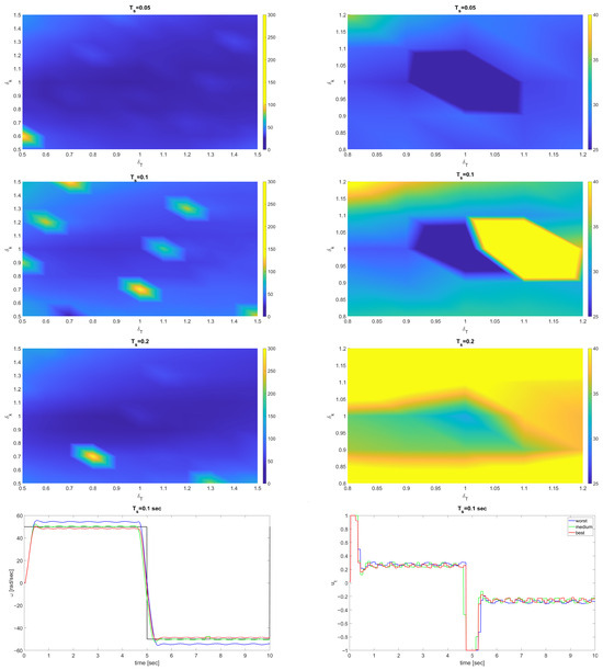
Figure 7. Surface of IAE for three sampling periods (zoomed in version in the right column), and time plots are below.

Regarding the comparison between the increase in performance indices for two configurations—the nominal one (${\delta }_k={\delta }_T=1$) and the worst one—between the configurations represented by the blue/red dots in the initial figures, the results concerning performance degradation are outlined in Table 2.

Table 2. Performance degradation in terms of $J_3$ index vs. $T_s$.

${\mathit{T}}_{\mathit{s}}\left[\mathbf{sec}\right]$	Nominal Parameters	Worst Configuration	Noted Increase
0.05	26.05	29.19	12.0%
0.1	27.83	32.77	17.7%
0.2	45.82	53.40	16.5%

It has turned out that the increase between nominal and worst configurations resembling parameter uncertainty resulted in an up to 18% increase in the performance indices, mainly connected to the slower dynamics of the closed-loop system, which is typically connected to robust control approaches.

7. Discussion and Conclusions

The presented results, concerning performance with uncertain data, clearly reveal that there is a great margin of uncertainty which is tolerated by the MPC framework to obtain a closed-loop system with a slight degradation in control quality.

The reason for this is that the prediction of the output takes into consideration not only the values of the signals from previous samples (i.e., signals not generated solely on the basis of the model) but also because of the optimization task solved, which basically enables one to obtain the best performance subject to the information available in a receding horizon framework.

This margin is narrowed when the sampling interval violates the rules of thumb of falling at least 10 sampling intervals in a dominating time constant, which has been shown in the conducted experiments.

Nevertheless, by extending the capabilities of a pure feedback with predictive features, one can expect slight performance degradation over a wide range of uncertainty. When the uncertainty is connected to the gain, steady-state errors appear and cannot be removed once there is no integral term in the open-loop system. This could potentially be easily removed once the MPC-like control law generates rates of changes in the control signal, not the control signal itself.

A similar behaviour has been observed in one of the prior stages of this research, using the same servo system, for which the IAE performance index has been calculated alike, and the green areas in Figure 8 are connected to a 30% increase in the performance index in comparison to the case when full knowledge concerning k and T are considered (dashed lines) in pole-placement control, and rotational velocity control [23].

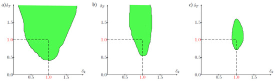
Figure 8. Areas of 30% performance degradation in pole-placement control with sampling intervals (a) $T_s=0.05\sec$, (b) $T_s=0.1\sec$, (c) $T_s=0.2\sec$.

This possibly leads the way to the further exploitation of adaptive control setups on the same platform since it tolerates uncertain knowledge concerning the nominal parameters of the plant, as it is not directly pushed to its limits, by imposing requirements connected to the dynamics of the closed-loop system, resulting in the control action saturating only when dynamic changes in the reference velocity take place. The other reason might be that the system is a relatively basic setup, with the dynamics described as a first-order system, resulting from [23].

Since in the configuration considered in this paper the model predictive control has been used, a natural question arises: what are the limitations of the method? Since the absolute value formulation is used, the non-smooth cost function impedes the theoretical analyses, especially related to stability proofs. The dynamics of the system might not be captured properly, as a linear programming problem; thus, potential extension to nonlinear systems is limited, unlike with nonlinear model predictive control approaches. Next, on a large scale, the linear programming might become problematic as per the number of slack variables introduced.

As future directions of the research, the authors clearly see the integration of integral action to mitigate steady-state errors observed under gain uncertainty, as well as extension of the LP MPC framework to nonlinear or time-varying models with uncertainty. This could also include the combination of LP MPC with machine learning for improved prediction or uncertainty modelling, as in [28], where the machine learning-enhanced control strategies are coupled with the MPC framework, for real-time optimization and control.

References

- Smith, R.S. Robust model predictive control of constrained linear systems. In Proceedings of the American Control Conference, Boston, MA, USA, 30 June–2 July 2004; Volume 1, pp. 245–250. [Google Scholar] [CrossRef]
- Recasens, J.; Chu, Q.; Mulder, J. Robust model predictive control of a feedback linearized system for a lifting-body re-entry vehicle. In Proceedings of the Collection of Technical Papers-AIAA Guidance, Navigation, and Control Conference, San Francisco, CA, USA, 15–18 August 2005; Volume 4, pp. 2952–2984. [Google Scholar] [CrossRef]
- Mousavi, H.; Ali Nekoui, M.; Derakhshan, G.; Hakimi, S.M.; Imani, H. A novel robust MPC scheme established on LMI formulation for surge instability of uncertain compressor system with actuator constraint and piping acoustic. Automatika 2024, 65, 1259–1270. [Google Scholar] [CrossRef]
- Pirouzmand, F.; Ghahramani, N.O. Robust model predictive control based on MRAS for satellite attitude control system. In Proceedings of the 3rd International Conference on Control, Instrumentation, and Automation, ICCIA, Tehran, Iran, 28–30 December 2013; pp. 53–58. [Google Scholar] [CrossRef]
- Chen, S.; Preciado, V.M.; Morari, M.; Matni, N. Robust model predictive control with polytopic model uncertainty through System Level Synthesis. Automatica 2024, 162, 111431. [Google Scholar] [CrossRef]
- Scokaert, P.; Mayne, D. Min-max feedback model predictive control for constrained linear systems. IEEE Trans. Autom. Control 1998, 43, 1136–1142. [Google Scholar] [CrossRef]
- Mayne, D.Q.; Kerrigan, E.C. Tube-based robust nonlinear model predictive control. IFAC Proc. Vol. 2007, 40, 36–41. [Google Scholar] [CrossRef]
- Horla, D.; Pinczewski, P. Deployment of a predictive-like optimal control law on a servo drive system using linear programming approach. Arch. Electr. Eng. 2023, 72, 1005–1016. [Google Scholar] [CrossRef]
- Yang, H.; Xi, D.; Weng, X.; Qian, F.; Tan, B. A Numerical Algorithm for Self-Learning Model Predictive Control in Servo Systems. Mathematics 2022, 10, 3152. [Google Scholar] [CrossRef]
- Wu, L.; Qu, J. Precision Cylinder Gluing with Uncertainty-Aware MPC-Enhanced DDPG. IEEE Open J. Control Syst. 2025, 4, 130–143. [Google Scholar] [CrossRef]
- Phuong, T.H.; Belov, M.P.; Van Thuy, D. Adaptive model predictive control for nonlinear elastic electrical transmission servo drives. In Proceedings of the 2019 IEEE Conference of Russian Young Researchers in Electrical and Electronic Engineering, ElConRus, Moscow, Russia, 8–31 January 2019. [Google Scholar] [CrossRef]
- Andrade, R.; Normey-Rico, J.E.; Raffo, G.V. Fast embedded tube-based MPC with scaled-symmetric ADMM for high-order systems: Application to load transportation tasks with UAVs. ISA Trans. 2025, 156, 70–86. [Google Scholar] [CrossRef] [PubMed]
- Gao, Y.; Huang, J.; Chen, L. Constrained Model Predictive Contour Error Control for Feed Drive Systems with Uncertainties. Int. J. Control Autom. Syst. 2021, 19, 209–220. [Google Scholar] [CrossRef]
- Yao, J. Model-based nonlinear control of hydraulic servo systems: Challenges, developments and perspectives. Front. Mech. Eng. 2018, 13, 179–210. [Google Scholar] [CrossRef]
- Pipino, H.A.; Adam, E.J. MPC for linear systems with parametric uncertainty. In Proceedings of the 2019 18th Workshop on Information Processing and Control, RPIC, Salvador, Brazil, 8–20 September 2019; pp. 42–47. [Google Scholar] [CrossRef]
- Fallahi, M.; Zareinejad, M.; Baghestan, K.; Tivay, A.; Rezaei, S.; Abdullah, A. Precise position control of an electro-hydraulic servo system via robust linear approximation. ISA Trans. 2018, 80, 503–512. [Google Scholar] [CrossRef] [PubMed]
- Sun, Y.B.; Guo, Q.D. Sliding mode robust tracking control for linear servo system based on RBF neural networks compensation. Kongzhi Lilun Yu Yingyong/Control Theory Appl. 2004, 21, 252–256. [Google Scholar]
- Bemporad, A.; Borelli, F.; Morari, M. Model predictive control based on linear programming: The explicit solution. IEEE Trans. Autom. Control 2002, 47, 1974–1985. [Google Scholar] [CrossRef]
- Biggs, M.; Hariss, R.; Perakis, G. Constrained optimization of objective functions determined from random forests. Prod. Oper. Manag. 2023, 32, 397–415. [Google Scholar] [CrossRef]
- Fiedler, F.; Karg, B.; Lüken, L.; Brandner, D.; Heinlein, M.; Brabender, F.; Lucia, S. do-mpc: Towards FAIR nonlinear and robust model predictive control. Control Eng. Pract. 2023, 140, 105676. [Google Scholar] [CrossRef]
- Rubagotti, M.; Patrinos, P.; Bemporad, A. Stabilizing linear model predictive control under inexact numerical optimization. IEEE Trans. Autom. Control 2014, 59, 1660–1666. [Google Scholar] [CrossRef]
- Britzelmeier, A.; Gerdts, M. A Nonsmooth Newton Method for Linear Model-Predictive Control in Tracking Tasks for a Mobile Robot with Obstacle Avoidance. IEEE Control Syst. Lett. 2020, 4, 886–891. [Google Scholar] [CrossRef]
- Horla, D. Robust Performance of Sampled-Data Adaptive Control of a Servo Drive. From Simulation to Experimental Results. J. Autom. Mob. Robot. Intell. Syst.-JAMRIS 2015, 9, 3–8. [Google Scholar]
- Maciejowski, J. Predictive Control with Constraints; Prentice Hall: London, UK, 2002. [Google Scholar]
- MOSEK Documentation. 2025. Available online: https://www.mosek.com/documentation/ (accessed on 1 October 2025).
- Gurobi 8 Performance Benchmarks. 2019. Available online: https://assets.gurobi.com/pdfs/benchmarks.pdf (accessed on 16 November 2025).
- Horla, D. C-code implementation of an adaptive real-time GPC velocity controller for a servo drive. In Proceedings of the 2016 17th International Conference on Mechatronics-Mechatronika (ME), Prague, Czech Republic, 7–9 December 2016; pp. 1–7. [Google Scholar]
- Jia, X.; Xia, Y.; Yan, Z.; Gao, H.; Qiu, D.; Guerrero, J.M.; Li, Z. Coordinated operation of multi-energy microgrids considering green hydrogen and congestion management via a safe policy learning approach. Appl. Energy 2025, 401, 126611. [Google Scholar] [CrossRef]
- Bitmead, R.; Gevers, M.; Wertz, V. Adative Optimal Control: The Thinking Man’s GPC; Prentice-Hall: Englewood Hills, OH, USA, 1990. [Google Scholar]
Disclaimer/Publisher’s Note: The statements, opinions and data contained in all publications are solely those of the individual author(s) and contributor(s) and not of MDPI and/or the editor(s). MDPI and/or the editor(s) disclaim responsibility for any injury to people or property resulting from any ideas, methods, instructions or products referred to in the content. |
© 2025 by the authors. Licensee MDPI, Basel, Switzerland. This article is an open access article distributed under the terms and conditions of the Creative Commons Attribution (CC BY) license (https://creativecommons.org/licenses/by/4.0/).