


Abstract
The Modular Multilevel Converter (MMC) has gained significant popularity over the past decade due to its versatility. The MMC features have been leveraged in numerous fields, including high-voltage DC transmission, electric vehicle power trains, motor drives, and wind energy conversion. In controlling the MMC, the circulating current (i.e., the current flowing through both the upper and lower converter arms without delivering power to the load) has consistently been the most critical variable. In early applications, it was perceived as a source of losses, but more recently, it has become evident that injecting a specific current could reduce voltage and energy ripples. This paper presents a theoretical framework, based on time-scale analysis, useful for modeling and controlling MMCs. The new approach is adopted for generating the circulating current reference, which is expressed as a linear combination of orthogonal functions. The goals are to decouple the control of the voltages of the upper and lower converter arms and manage additional harmonic components of the circulating current for voltage ripple reduction on module capacitors. The simulations and experimental results demonstrate the effectiveness of the proposed control strategy.
1. Introduction
The Modular Multilevel Converter (MMC) was proposed by Prof. Rainer Marquardt in the early 2000s and has since emerged as one of the most intriguing Voltage Source Converter (VSC) topologies [1,2]. Its versatility and scalability to different power levels have made it a significant player in various application fields, including high-voltage DC transmission [3,4], motor drives [5,6], electric vehicle power trains [7], photovoltaic generation [8,9], wind energy conversion [10], and fast charging stations [11,12]. Since its inception, the MMC has sparked global interest in the power electronics community. Many research threads have been initiated surrounding the MMC, including the investigation of alternative converter configurations, theoretical models for the construction of control architectures, the analysis of numerous potential modulation techniques, the study of fault management, and the optimization of hardware [13,14].
In multilevel inverters, capacitors are usually adopted to create the different voltage levels needed for the converter operation, but keeping the voltages across them balanced may be challenging. In contrast to other multilevel converter topologies, the MMC provides a simpler approach to balancing capacitor voltages.
A three-stage control structure, comprising internal capacitor voltage balancing, current regulation, and voltage or energy control, and based on proportional-integral (PI) or proportional-resonant (PR) regulators, is widely adopted [15,16,17]. This approach works properly in case of applications with a fixed ac frequency, such as HVDC systems.
Alternative control methods, which are particularly effective for applications where the ac frequency is variable (motor drives), are based on sliding mode [18,19] and model predictive control [20,21,22]. Recently, a different control method, based on linear quadratic regulators, was proposed in [23].
The behavior of the capacitor voltage strongly depends on the current circulating between the arms and the voltage sources. This circulating current, also known as differential current, has been studied since the beginning of the MMC history, owing to its impact on the voltage balancing and the overall losses of the converter [14,24,25]. Furthermore, since this circulating current flows in both arms of a leg of the converter, the two arms are coupled from a control system point of view. Usually, the efforts are directed towards suppressing this current [26]. However, studies have demonstrated that a circulating current with specific harmonic content can benefit the MMC. This approach reduces the voltage ripple on the capacitors, together with the ripple and the rms value of the capacitor currents, and then the cost of the converter, enabling the use of smaller capacitors [27]. However, the increased rms value of the arm currents results in increased power losses.
The strategies employed to generate the circulating current reference rely on controlling the total and differential energies. However, this approach maintains the arms in a state of interdependence, thus precluding the possibility of controlling one arm independently of the other.
This paper presents a new theoretical framework useful for modeling and controlling MMCs that allows the energy management of the two arms to be decoupled. The approach is different from the standard one based on the control of the total and differential energies, although the performance is similar. By exploiting the concepts of different time scales and orthogonal functions, already proposed in [28,29], it is possible to detach the circulating current into two different components so that each component affects only one arm. In addition, in this paper, the new theoretical approach is adopted to explain how a second-order harmonic component in the circulating current helps decrease the total energy ripple, reducing the oscillations of the capacitor voltages [27]. A similar approach, based on general averaging techniques, has been applied to three-phase MMCs for drive applications [30].
The main contributions of the paper are listed hereafter:
- Definition of a coherent mathematical framework for the analysis and control of MMCs, which is based on the concepts of different time scales and orthogonal functions;
- Definition of an alternative approach for describing the circulating current, potentially enabling new ways to design and understand control strategies for MMCs;
- Proposal for a new control scheme capable of decoupling the control of the upper and lower arms, by inherently separating the variables with slow dynamics, such as the arm energies, from those with fast dynamics, such as the output voltages and currents;
- Demonstrating the ability of the proposed approach to manage properly additional oscillating components of the circulating current.
A simulation model was developed to demonstrate the efficacy of the proposed strategy. Additionally, experimental tests were conducted on an MMC prototype. The simulation and experimental results are aligned, thereby substantiating this approach as a viable alternative to the prevailing energy control methodology. This approach effectively decouples the control of the arms and reduces the total energy ripple and the voltage ripple on the capacitors.
In this paper, the proposed approach is applied to a single-leg MMC for the sake of clarity and to highlight the fundamental principles of the framework. However, since the formulation of the circulating current is performed independently for each leg, the method can be directly extended to three-phase and multi-phase MMCs (number of phases greater than three, for propulsion systems) without requiring special modifications.
This paper is structured as follows: after the introduction, Section 2 introduces the time-continuous model of an MMC, presenting the fundamental concepts. Section 3 shows the fundamental equations of the converter, while Section 4 focuses on the control, the mathematical model, and the new proposed strategy. Finally, Section 5 presents the control logic for implementing the developed strategy. Section 6 is dedicated to the simulation model built to prove the effectiveness of the decoupling control based on the concept of orthogonal functions. Section 7 presents the experimental results of an MMC prototype controlled through the proposed solution, and Section 8 presents the conclusions of this work.
2. Continuous-Time Model of an MMC
There are numerous MMC topologies [31,32], yet they all share several fundamental characteristics. Each topology comprises a series of identical cells called submodules (SM). A linear arrangement of these submodules constitutes an arm. Each arm of the converter contains an equal number of submodules. The connection of two arms (commonly referred to as the upper and lower arm) forms a leg. An MMC may consist of one or multiple legs.
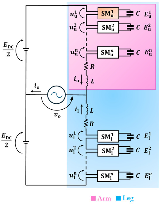
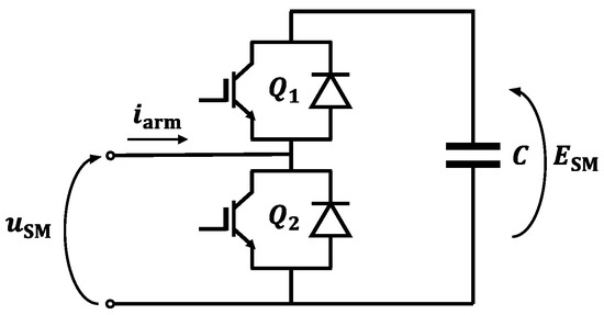
The basic topology of an MMC (depicted in Figure 1) is constituted by a single leg. The input voltage source is the DC-link voltage , the output current is , and is the output voltage. As shown in Figure 2, the submodules (SMs) consist of a half-bridge leg made up of two IGBTs and two antiparallel diodes, along with a capacitor connected in parallel.
Figure 1.
MMC basic topology.
Figure 2.
Submodule architecture comprising a half-bridge connected in parallel to a capacitor.
An inductor is placed before the connection point with the other SMs to address the voltage imbalance that arises from switching operations between the two arms.
The voltage generated by each leg results from the combination of its SM voltages. Accordingly, the proper switching configuration enables synthesis of the desired output voltage. However, it is essential to maintain the voltage balance of the SM capacitors. A sorting algorithm embedded in the control architecture determines which SMs are inserted or bypassed in each sampling interval to ensure a balanced voltage across all SMs [33].
Specific assumptions must be made to develop a mathematical model of the converter that is both simplified and accurate. The first assumption for a single-phase half-bridge MMC topology is that the SMs belonging to the same arm are perfectly synchronized in their charge/discharge operations and have a perfect voltage balance at any instant. This assumption allows all the SMs of an arm to be replaced by a single equivalent SM. Consequently, the model can correctly describe the behavior of the converter regardless of the number of arm submodules. The other two assumptions are that at least two orders of magnitude separate the fundamental output frequency and the switching frequency, and due to the large number of SMs, the resolution of the output voltage is much smaller than the voltage amplitude.
3. MMC Equations
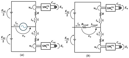
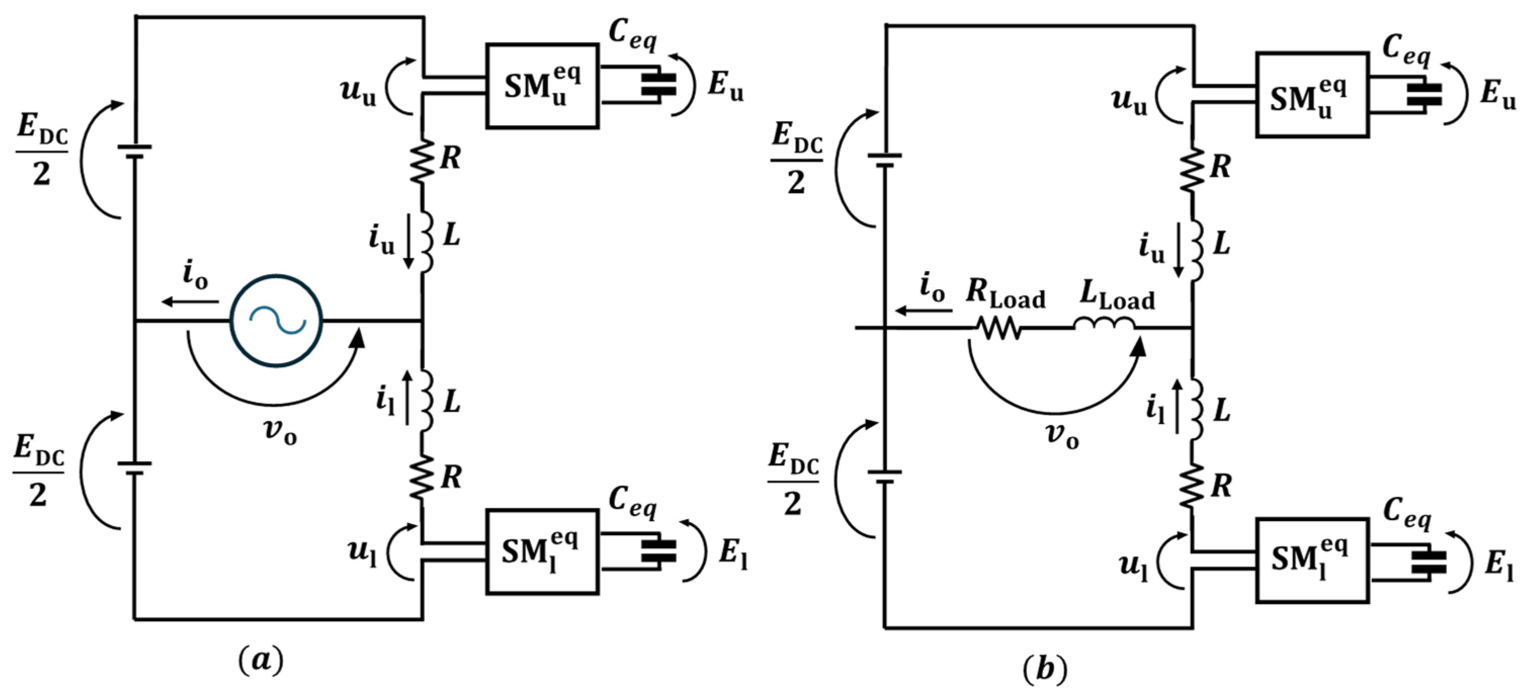
The schematics depicted in Figure 3 can be used as a starting point to derive the equations of the two arms of the MMC:
where and denote the inductance and resistance of the converter arm, respectively, and are the currents of the two arms (the subscript “u” stands for “upper” and “l” for “lower”), and are the capacitor voltages of the two equivalent submodules and , and are the modulation indexes produced by the control logic to operate the SMs, is the DC voltage, and is the output voltage. If the converter is connected to the grid, the output voltage can be a given quantity, such as in Figure 3a. Otherwise, it may depend on the load, such as in Figure 3b.
Figure 3.
Simplified schemes of an MMC: (a) The converter is interfaced with a sinusoidal voltage source; (b) The converter supplies a passive load.
For the upper and lower equivalent SMs, the equations relating the capacitor currents ( and , respectively) to the capacitor voltages ( and , respectively) are as follows:
where denotes the equivalent capacitance of each arm obtained as the series of all the arm capacitances.
The output current, denoted by , is obtained by summing the current contributions of the two arms. It can be expressed as follows:
Another fundamental current that must be considered in an MMC is the circulating current , which is defined as the differential current between the two arms within the same converter leg.
The circulating current flows through its corresponding leg and the DC source. Therefore, it does not affect the output quantities. Equations (5) and (6) can be manipulated to express the currents and as functions of the currents and , resulting in the following equations:
The dynamic equations for and are derived by adding and subtracting (1) and (2), while taking (5) and (6) into account:
where
The voltages and are formulated as functions of the SM duty cycles in (11) and (12), thereby demonstrating the correlation between these variables.
Upon determining the expressions for and , the modulating signals are obtained through the inversion of (11) and (12).
Assuming a passive load scenario, as shown in Figure 3b, it is necessary to include the equation of the load in the system model:
where and represent the load resistance and inductance, respectively.
The control equation for the load current, dependent on both load and converter parameters, results from the combination of (9) and (15):
Load current control may be formulated using (9) or (16) depending on whether is an impressed voltage or not. In the latter case, can be estimated by means of (15).
4. MMC Control and Proposed Solution
MMC control strategies are typically developed to fulfill two primary objectives. The first is to ensure the prescribed output quantities for and , and the second is to stabilize submodule voltages within safe operating bounds, minimizing ripple amplitude. These two goals necessitate the control of three variables: , , and .
Given that the only control variables of the system are the two modulation indexes and , the control strategy is not straightforward. As previously stated in (9) and (10), it can be seen that and can be controlled by the voltages and , defined in (11) and (12), respectively. It is worth highlighting that a significant distinction exists between the two currents, and . This distinction pertains to the generation of their respective references because is a known quantity, while must be selected. Subsequent sections will detail the influence of the circulating current on the total energy stored in the SM capacitors and its role in mitigating their voltage imbalance.
4.1. Control of the Capacitor Voltages
The total electromagnetic energy in each arm, for the upper and for the lower, can be formulated as the sum of the magnetic energy stored in the arm inductors and the electrostatic energy of the equivalent capacitors:
It should be noted that, for a properly designed MMC, the energy stored in the arm inductors is negligible compared to that stored in the arm capacitors.
The time derivatives of and , assuming negligible the inherent resistances of the arm inductors, can be formulated as follows:
Replacing and using the expressions found in (7) and (8), it yields:
where
Equations (21) and (22) describe the time derivatives of the energy stored in the upper and lower arms as the sum of two components: one proportional to the output current , and the other to the circulating current . The key difference is that the former term cannot be controlled, being inherently tied to , which follows a prescribed reference, whereas the latter is controllable via using the expression shown in (10); thus, becomes the control variable for managing the capacitor voltages.
4.2. Two Time-Scale Analysis
The arm energies and exhibit harmonic components at frequencies that are integer multiples of the output frequency , as illustrated in (19) and (20). This results from their dependence on and , which vary sinusoidally. Moreover, the arm energies exhibit a long-term, non-periodic trend, commonly referred to as a secular variation. To distinguish between periodic variations and secular terms, the technique of multiple time-scale analysis, commonly used in perturbation theory, can be adopted.
For the sake of simplicity, only is considered in what follows because the same reasoning can be repeated for . Using the multiple-scale analysis approach, is represented as a function of two angular variables, and , which evolve on distinct time scales and are considered independent:
with representing the slow variable and the fast one.
Assuming the slow-varying component has a frequency band [0, ], where << , and defining as the small number defined as the ratio of and , the variables and are related to time as follows:
Furthermore, is periodic with respect to :
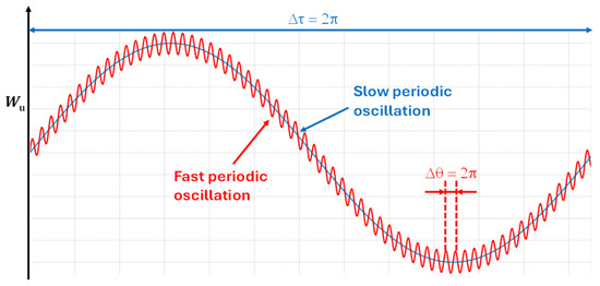
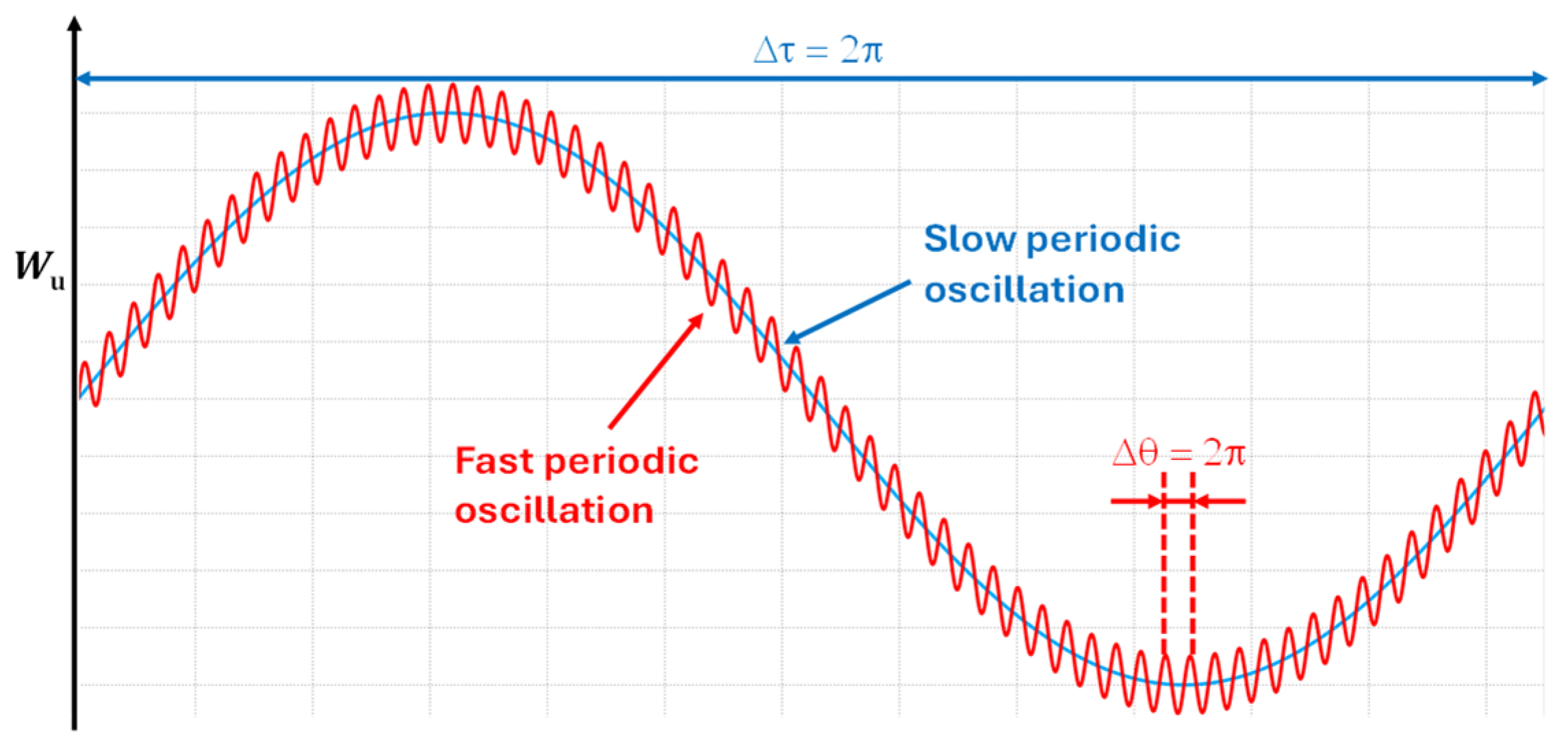
Figure 4 shows the meaning of and .
Figure 4.
Fast and slow time scales.
Considering the chain rule, the time derivative of becomes:
By substituting , multiplying both sides of (21) by ε and taking (29) into account, yields:
For small values of , can be expanded in powers of following standard perturbation theory [34,35], with the underlying assumption that the th term becomes vanishingly small compared to the nth term as :
Since is a periodic function of , and must be periodic functions too.
Substituting (31) into (30) and matching terms of equal powers of yields the following equations for the first two orders:
Equation (32) indicates that is independent of the fast variable , thereby characterizing the slow-varying component of the arm energy, also known as the secular term. Due to its significantly shorter period compared to the slow transients, the contribution from the fast oscillation may be considered negligible. Consequently, the derivative of with respect to time is given by:
The right-hand side of (34) is obtained by integrating both sides of (33) with respect to over the interval [, ]. Since is a periodic function of , the integral of is zero, and (34) becomes as follows:
A similar expression can be found for by repeating the same steps:
Equations (35) and (36) can ultimately be reformulated using time as the integration variable, by taking (27) into account:
where is .
Equations (37) and (38) provide explicit expressions for the time derivatives of the slowly varying components of the arm energies, highlighting their dependence on the average power exchanged by the SMs over the period . Equations (37) and (38) can be used instead of (21)–(22) to synthesize a stable control system.
4.3. Orthogonal Functions
In a vector space with inner product , two functions, and , are orthogonal when their inner product equals zero.
The integral operator defined in (39) possesses the properties of linearity, symmetry, and positive definiteness. Hence, it defines an inner product on the space of real periodic functions over the interval [],
Equations (35) and (36) can be rewritten using (39) as follows:
Among the variables in (40) and (41), is the sole independent variable available for controlling the arm energies. This implies that the two arm energies are interdependent and cannot be regulated independently.
To enable independent control of the two arms, may be represented as a linear combination of two distinct functions, and . While exerts influence on the arm energy of the upper arm, affects only the arm energy of the lower arm:
where the quantities and are parameters depending on the slow time variable . The unit measure for and is [V], while and are measured in [W−1].
It is helpful to choose and , which can be arbitrarily selected, mutually orthogonal to the voltage functions and , as follows:
where is an arbitrary non-zero constant with the dimension of power [W].
Combining (40)–(42) yields a system of two decoupled equations:
Equations (44) and (45) indicate that and may be considered independent variables, each governing the arm energies with slow dynamic behavior.
4.4. Reciprocal Functions
Equation (42) indicates that, to achieve decoupled control of the arm energies, must lie within the linear span of and . The basis is said to be reciprocal to the basis ( ) since (43) ensures and are orthogonal to and , respectively.
In (42), the functions and represent the so-called covariant components of .
The explicit forms of and can be derived under the assumption that both can be expressed as linear combinations of and :
The coefficients and in (46) are usually referred to as contravariant components of .
To determine the explicit values of the coefficients , one must solve the matrix equation resulting from the combination of (46) and (43) for :
The solution of (47) is as follows:
Given that is constant and exhibits sinusoidal behavior in steady-state, the values of the coefficients can be determined by substituting (23) and (24) in (48):
where is the root mean square value of the output voltage.
Then, and can be rewritten by combining (23), (24), (49), (50), and (46) as follows:
In summary, the reference value for can be determined using (42), where and are independent functions selected to regulate the arm energies as prescribed by (44) and (45), and and are given by (51) and (52).
It should be noted that the definition of the orthogonal functions and , able to ensure decoupling, is not unique. The simplest solution is adopted in this paper, where a linear combination of and is assumed in (46).
4.5. Circulating Current and Total Energy Ripple
Equation (42) does not provide all the expressions of the current but only those that affect the arm energies. Such a consideration gives rise to the question of the potential integration of other components of the current that do not interfere with the control of the arm energies but may somehow improve the converter performance.
In a more general form, in (42) can be redefined as follows:
where is introduced as a current component that should not influence the evolution of and . For this reason, must be chosen orthogonal to and .
The fast-varying component of the arm energy can be derived by combining (33) and (34) as follows:
Assuming the slow-varying component of the arm energy is constant, its time derivative vanishes. Accordingly, the expression for the fast-varying component of takes the following form:
The same considerations that lead to (55) can be repeated for the energy of the lower arm.
By adding (55) and (56), the derivative of the fast-varying part of the leg total energy can be expressed as follows:
The term in (53) can be employed to attenuate the fluctuations in , resulting from the oscillating component of output power . Incorporating a suitable second-order harmonic into the circulating current is acknowledged as an effective approach that ensures a very significant reduction in total energy fluctuation and near minimal fluctuation in arm energies and [27].
Assuming sinusoidal output voltage and current, the resulting output power includes a harmonic component at frequency .
where is the output phase angle and is the rms value of the output current.
Replacing (53) and (58) in (57) leads to the following equation:
The quantities and are slow-varying functions of , whose steady-state values can be obtained from (44)–(45).
Taking into account (23)–(24) and (60)–(61), (59) simplifies under the steady-state condition of the slow-time leg energy component as follows:
Hence, to reduce the fluctuation of the total energy, the current must be equal to the following quantity:
The expression for in (63) is orthogonal to and , and thus does not influence the slow-time components of the arm energies.
The injection of has a positive effect on the cost of the converter, as it reduces the capacitor voltage oscillations, alongside the ripple and the rms value of the capacitor currents, making it possible the use of smaller capacitors. However, it must be recognized that the additional current component has the negative effect of increasing the power losses in the MMC. The opportunity to inject the current , in a cost/benefit analysis, depends on many factors and is beyond the scope of this paper.
5. Control Scheme
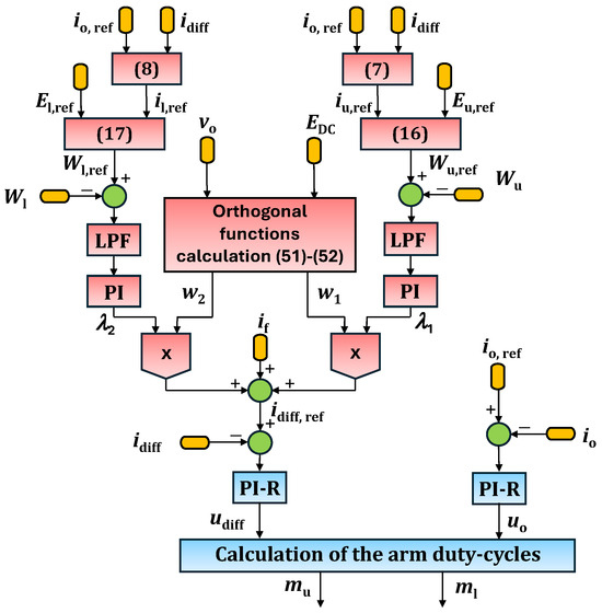
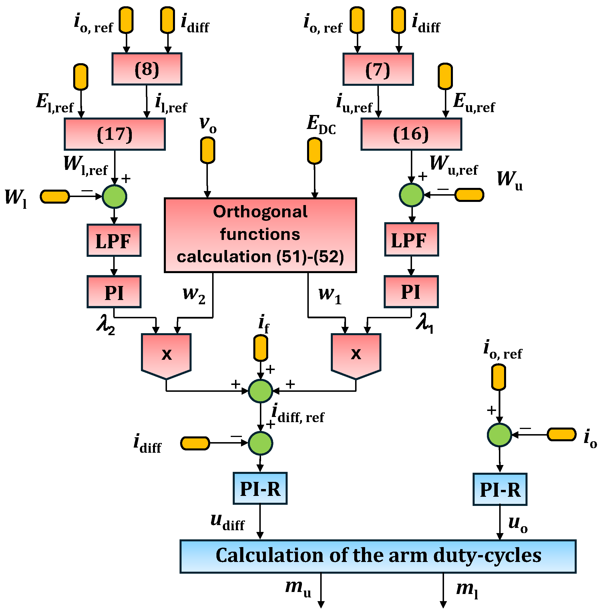
Figure 5 depicts the control logic architecture resulting from the analysis in the preceding section. The reference signals of the arm energies , are compared with the actual values , . The reference signals are evaluated by (17) and (18), whose inputs are the reference signals of the capacitor voltages , and of the arm currents , . The reference values of the arm currents can in turn be obtained by using (7) and (8), starting from the reference value of the output current and the actual value of circulating current, and , respectively. With a similar procedure it is possible to determine the actual values of the arm energies , starting from the measured values of voltages and currents.
Figure 5.
MMC control block diagram.
The slow-varying components of the tracking errors of the arm energies are evaluated by two low-pass filters (LPF blocks) and used as input of two PI regulators (PI blocks), which define the signals and . As shown in (53), and together with the orthogonal functions and , can be used to calculate two of the three terms of the reference signal of the circulating current . The orthogonal functions and can be evaluated starting from the measurements of and and implementing (51) and (52).
After computing the third term of the circulating current using (63), or by extracting the output power oscillating component divided by , the reference value of the circulating current can be determined according to (53).
Subsequently, the current setpoints and are compared to and and tracked by two multi-resonant PI regulators (PI-R blocks), which provide the voltages and used to generate the modulation indexes and by means of (13)–(14), taking the measured values of and into account. The multi-resonant PI controllers, specifically designed with resonant frequencies and , are necessary to ensure perfect current tracking in a steady-state because the reference signals contain harmonics at these frequencies.
The computational complexity required by the presented control scheme is commensurate with that demanded by conventional control algorithms, as the number of filters and regulators (PI/PI-R) that need to be implemented is similar. However, it should be noted that thanks to the use of multi-Resonant PI regulators, the proposed control scheme does not require the implementation of time-consuming reference frame transformations, which are necessary in other cases.
The control scheme is readily adaptable to a three-phase MMC configuration and is intrinsically robust against unbalanced three-phase grids as the focus is the definition of the circulating current independently in each leg. Furthermore, it should be noted that a low-level balancing algorithm, essential to maintain the balance of the voltages of the SM capacitors, is embedded in the control architecture [33].
6. Simulation Outcomes
A MATLAB Simulink (version R2024b) simulation model has been developed to demonstrate the effectiveness of the control strategy and verify that the use of orthogonal functions for generating the circulating current reference enables decoupled control of the two arms. This model emulates the operation of an MMC comprising a single leg and three SMs per arm; the SMs are constructed from a half-bridge leg with a capacitor in parallel. The converter feeds an L-R load. The main parameters utilized in the simulation model are listed in Table 1.
Table 1.
Main Parameters of the System.
The simulation starts in balanced conditions (i.e., ) without the contribution of (i.e., ). The injection of is enabled once the system reaches the steady-state. Furthermore, a step variation is applied to the voltage reference of the upper arm capacitors after the end of the transient.
Figure 6, Figure 7, Figure 8, Figure 9 and Figure 10 show the main outcomes of the simulations. As detailed in Section 4.5, introducing a component at twice the fundamental frequency with an appropriate phase angle into the circulating current helps mitigate total energy oscillations. Figure 6 shows that the injection of reduces the ripple of the total energy by 64%.
Figure 6.
Mitigation of total energy ripple resulting from component injection.
Figure 7.
Effect of component injection on arm currents and voltages.
Figure 8.
Converter response to a 10% step reduction in the setpoint . Waveforms of , (upper traces). Waveforms of , (lower traces).
Figure 9.
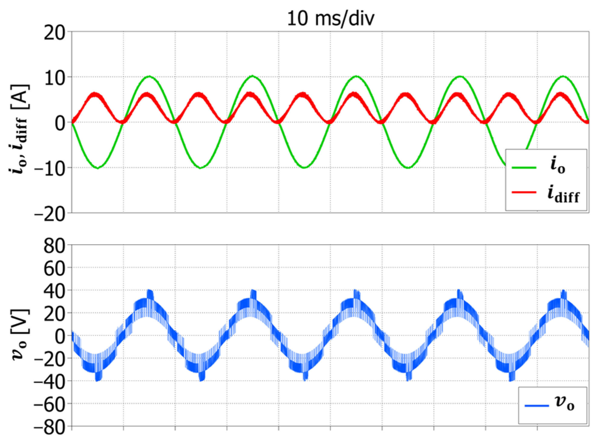
Converter behavior at steady-state. Waveforms of , (upper traces) and (lower trace).
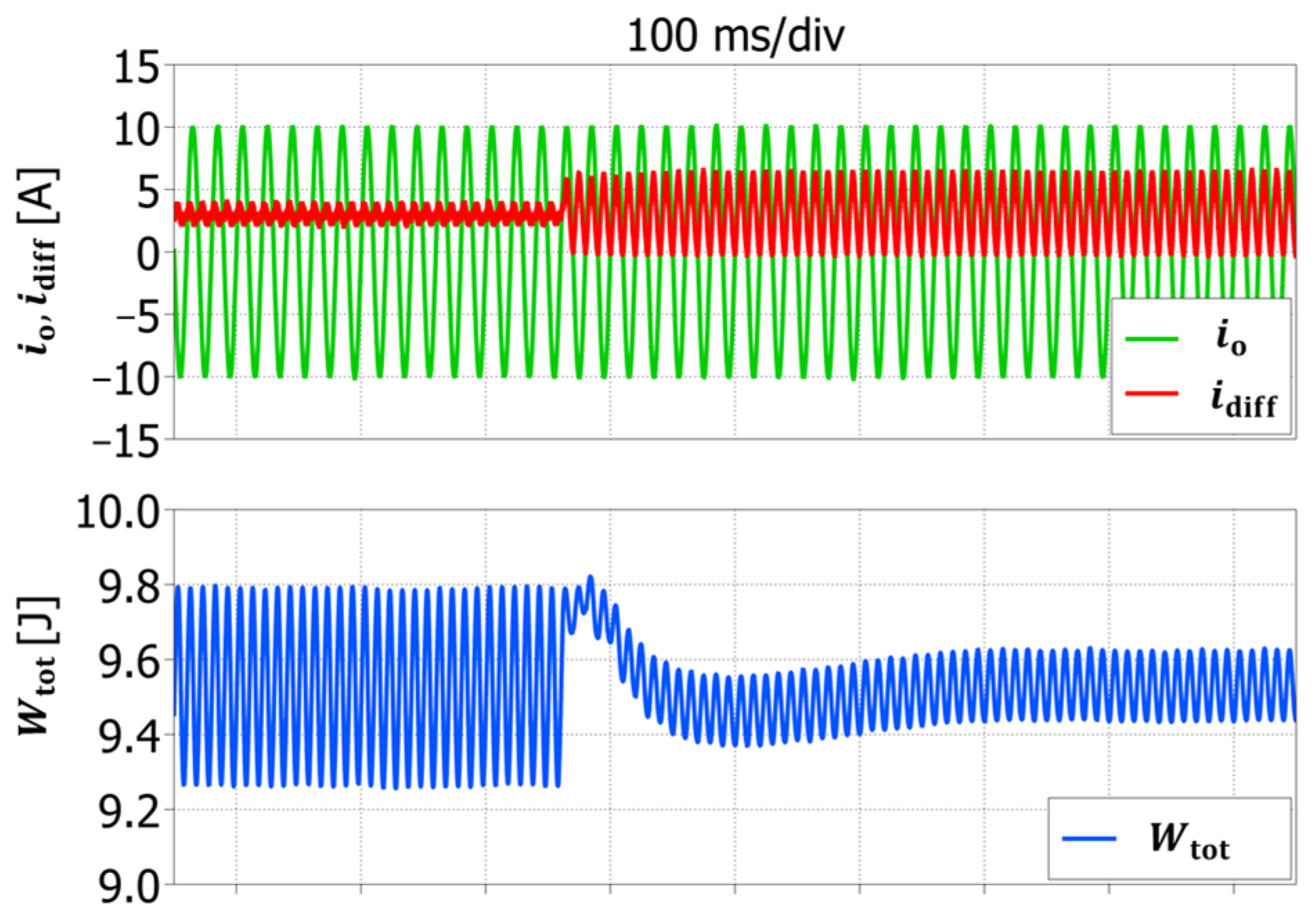
Figure 10.
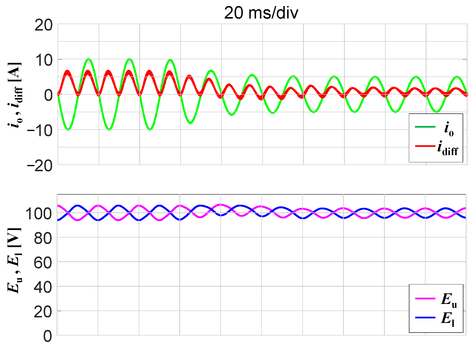
Waveforms of , (upper traces) and , (lower traces) during a step variation in the output current.
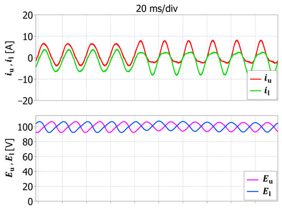
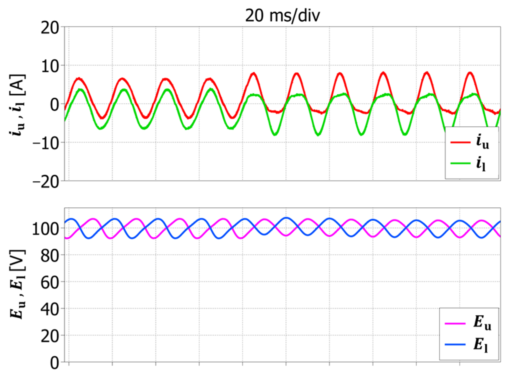
The impact on the arm capacitor voltages, shown in Figure 7, is less significant but still appreciable. The reduction in the peak-to-peak capacitor voltages is 13%, from 14.4 V to 12.9 V.
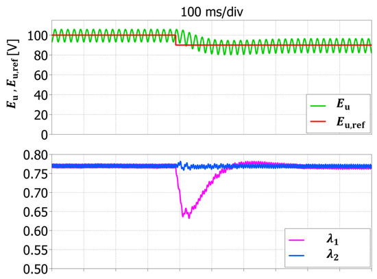
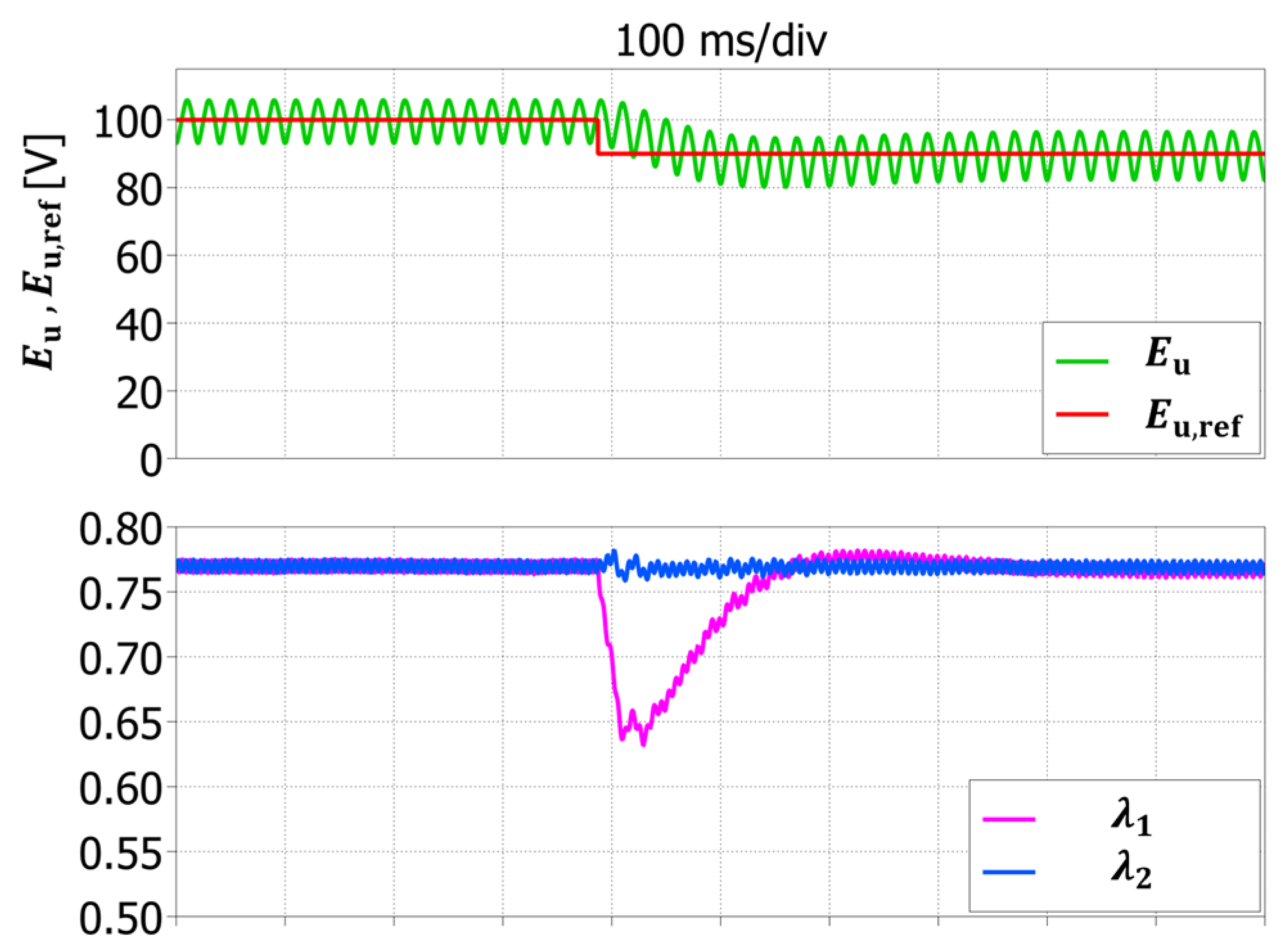
Figure 8 shows the converter behavior when the DC upper arm voltage reference is decreased by 10% of its nominal value, i.e., from 100 V to 90 V.
This variation affects only the parameter , which is related to the upper arm and exhibits a significative variation, while the parameter , linked with the lower arm, remains stable. The effectiveness of the proposed strategy in decoupling the control of the two arms is confirmed by this result.
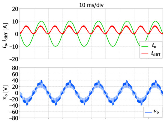
Figure 9 shows the output quantities in steady-state balanced conditions, with = 100 V, a reference output current with amplitude of 10 A and frequency 50 Hz, when the injection of is enabled. Expectedly, analysis confirms that the circulating current comprises a dc component and an oscillatory component at twice the output frequency. The output current is practically sinusoidal, whereas the output voltage has the typical multilevel waveform.
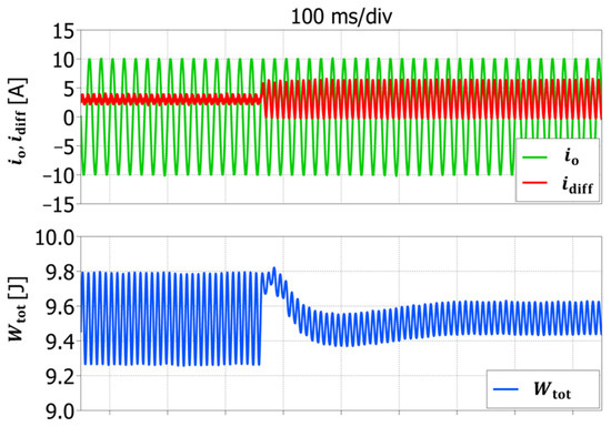
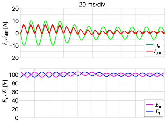
To better assess the behavior of the presented control system under transient conditions, the results of a numerical simulation carried out during a step change in the amplitude of the output current (from 10 A to 5 A), with a constant reference value of the arm capacitor voltages (100 V), are illustrated in Figure 10.
As expected, the output current amplitude decreases rapidly, whereas the waveform of the circulating current varies both in terms of average value and in terms of amplitude of the second harmonic, in agreement with (63).
Furthermore, the arm capacitor voltages maintain a stable behavior, with small oscillations around the reference value.
7. Experimental Results
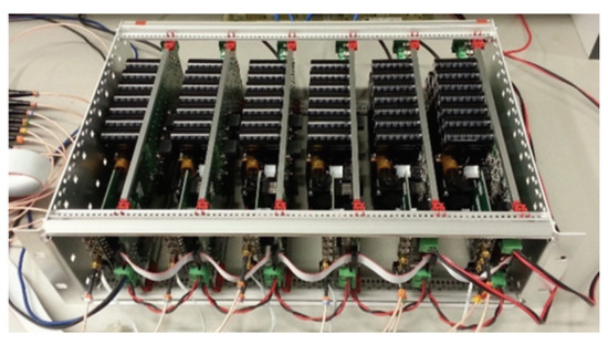
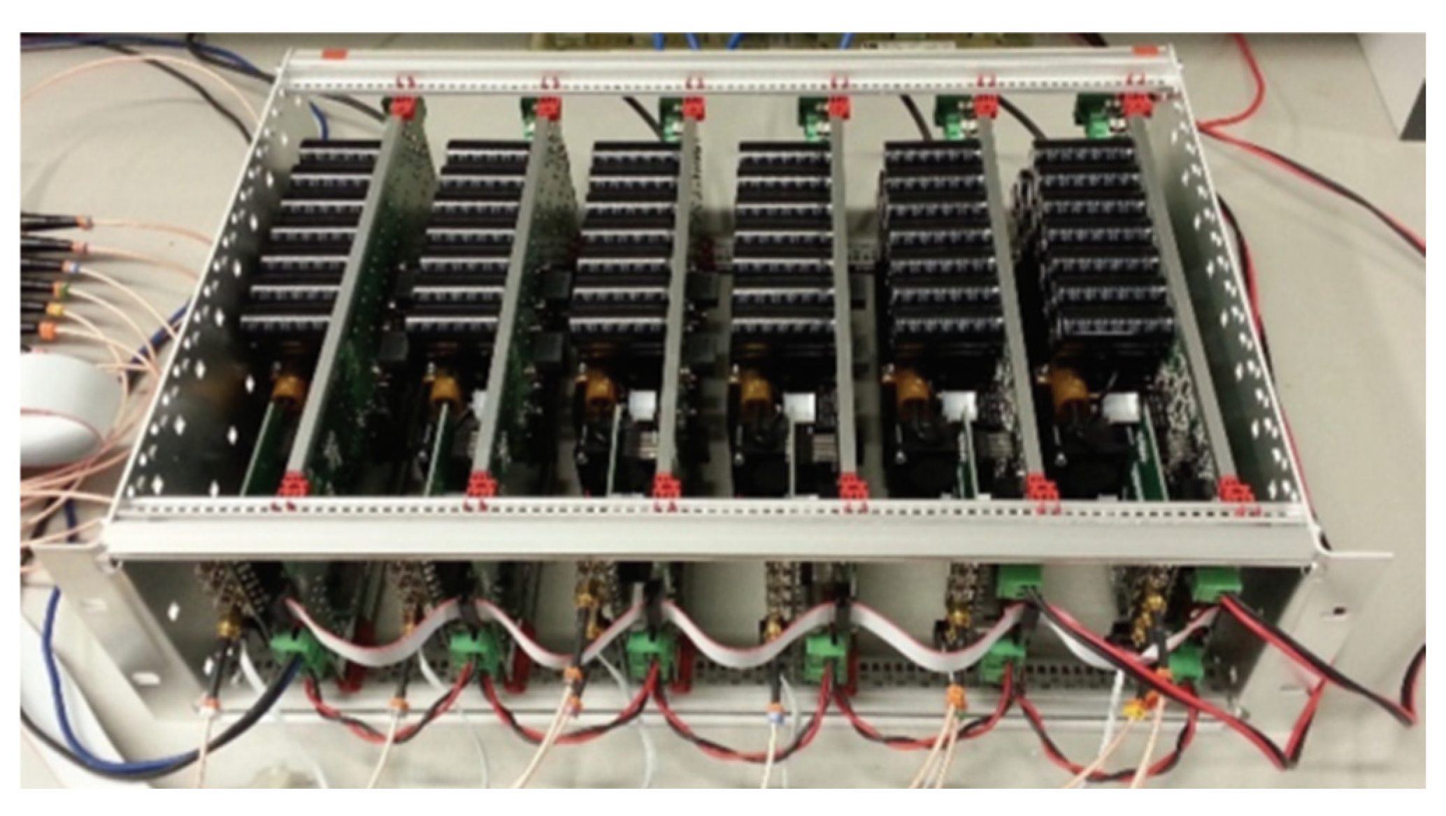
To validate the developed control strategy, a single-leg MMC prototype, depicted in Figure 11, has been built. The experimental tests replicate the simulations. The SM capacitances, arm inductances, and arm resistances have been sized to match the values listed in Table 1, and the control parameters and references have been set to the same values as the corresponding values used in the simulation model. In particular, each submodule uses 600 V, 30 A IGBTs (STMicroelectronics STGW30H60DFB) and 19 electrolytic capacitors connected in parallel (150 µF, 450 V). The PWM signals of each module and the voltage and current feedback are exchanged with a centralized control platform based on a Texas Instruments TMS320F28335 DSC. The control algorithm is implemented in C language, the control cycle and switching frequency are synchronized and executed at a frequency of 10 kHz.
Figure 11.
MMC prototype comprising six submodules employed for experimental testing.
The small-scale converter prototype available in our laboratory is based on Si IGBTs, but new wide bandgap semiconductors for medium voltage applications are available nowadays. The substitution of Si IGBTs with SiC MOSFETs would certainly improve the converter performance in terms of much higher switching frequency available, lower conduction and switching losses, and better heat dissipation. Note that the adoption of SiC MOSFET would not affect the validity of the presented theoretical framework or the proposed control scheme.
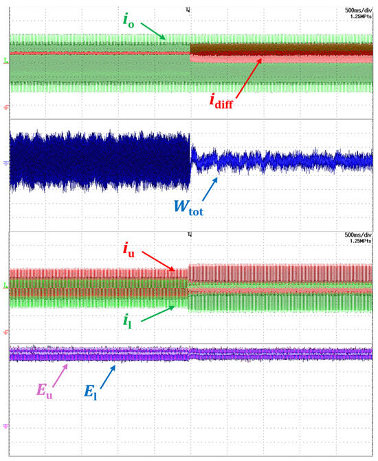
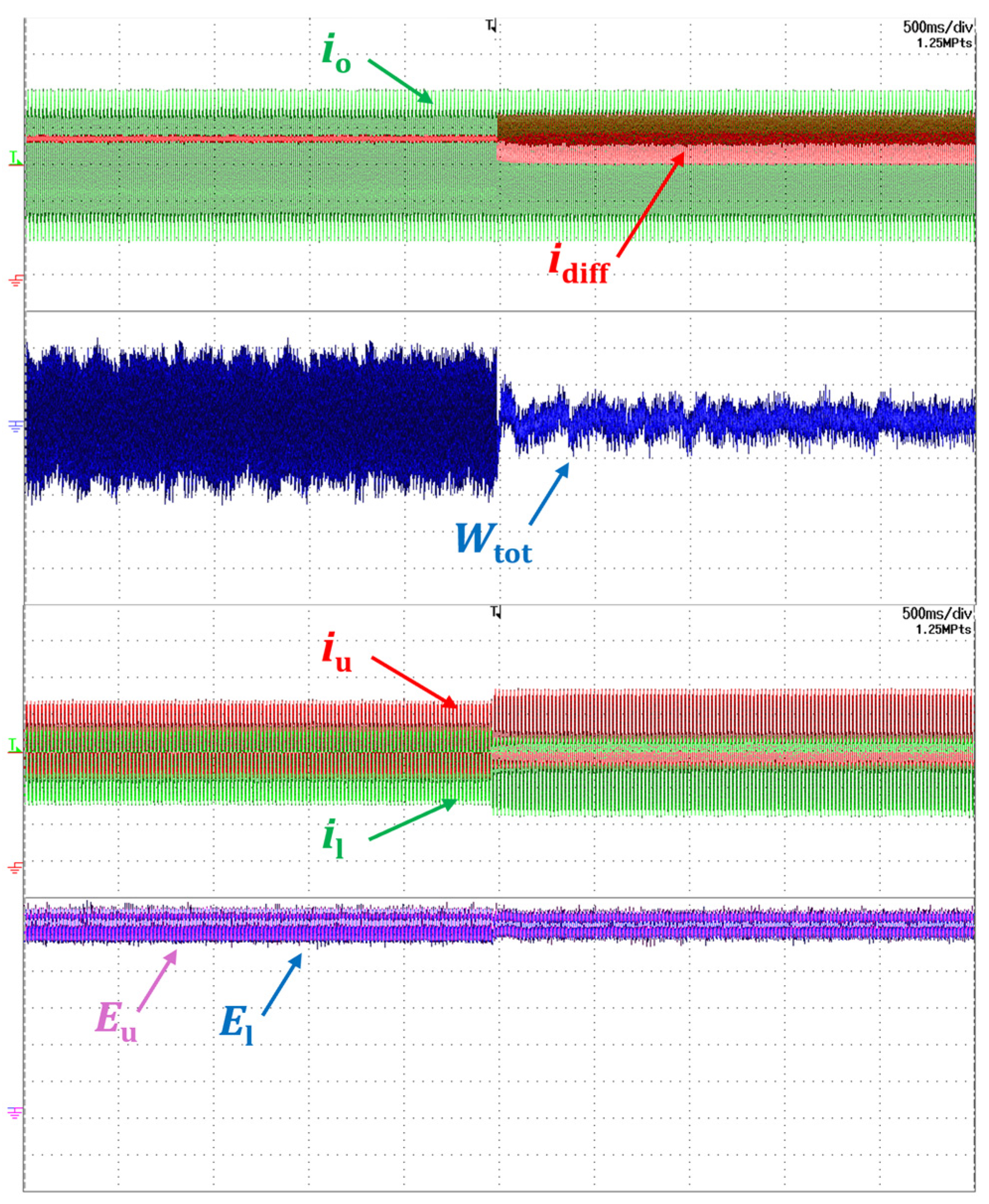
Figure 12 shows what happens when the converter operates in steady-state balanced conditions ( = 100 V), and passes from zero to the value given by (63) at the midpoint of the time interval displayed. The effects of the injection are clearly recognizable. The circulating current oscillates at twice the fundamental frequency, the mean value of the total energy remains unaltered, whereas its ripple significantly reduces. Furthermore, the rms value of the arm currents increases, and the ripple of the capacitor voltages and , as expected, decreases slightly.
Figure 12.
Converter response to injection. From top to bottom: output current (5 A/div, in green); circulating current (5 A/div, in red); total energy (200 mJ/div, in blue, AC coupling); upper arm current (5 A/div, in red); lower arm current (5 A/div, in green); upper arm voltage (20 V/div, in purple); lower arm voltage (20 V/div, in blue).
The waveform of the total energy after the injection in Figure 12 can be compared with the equivalent waveform obtained by numerical simulations in Figure 6. The amplitude of the peak-to-peak ripple is nearly identical (0.19 J in Figure 6, 0.2 J in Figure 12).
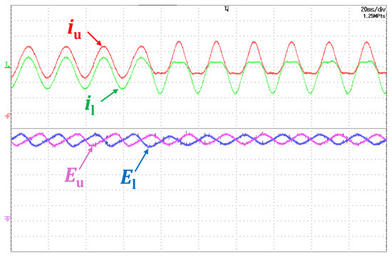
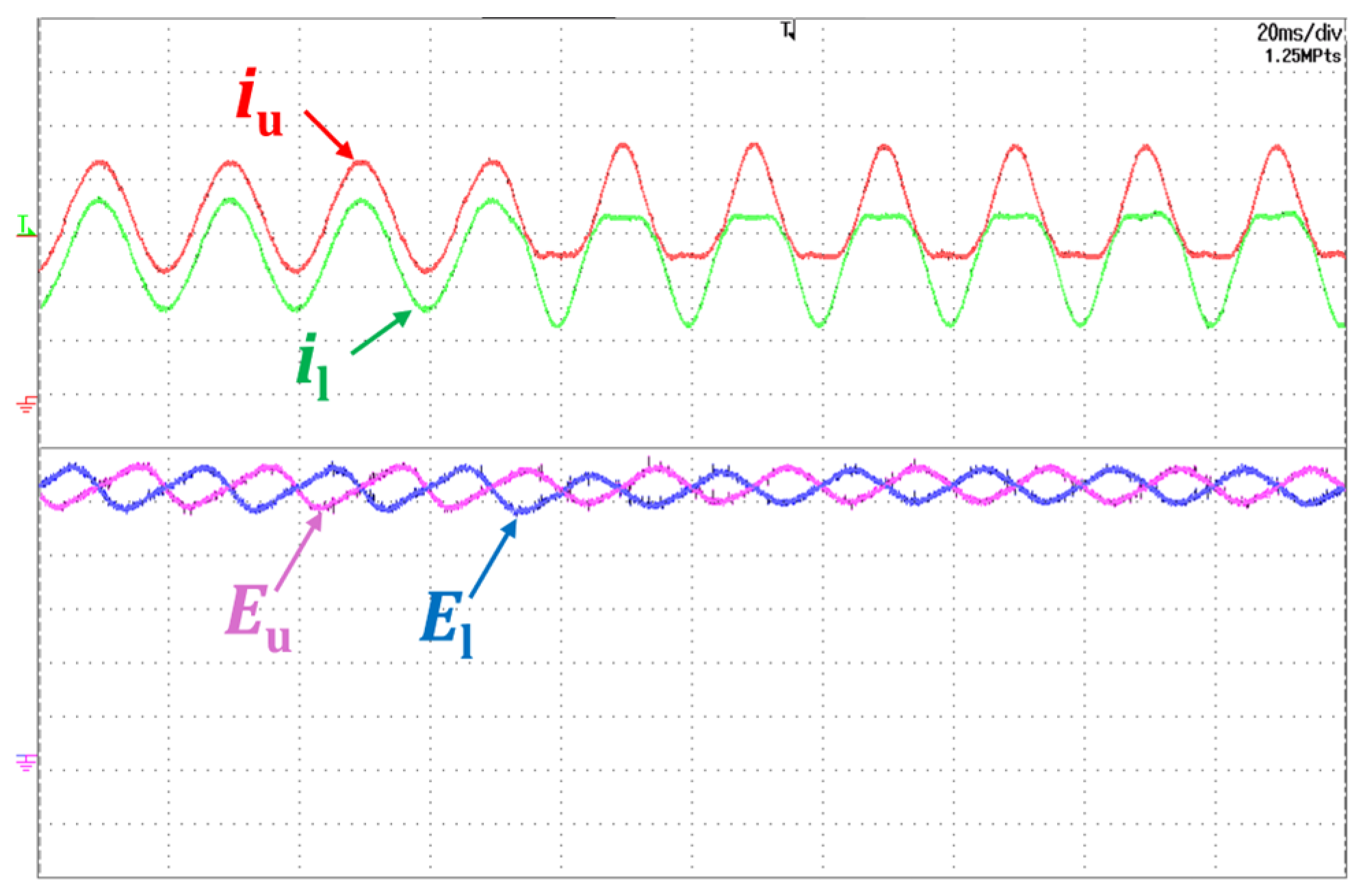
The tests shown in Figure 13 replicate those in Figure 12, with the time scale adjusted to 20 ms/div from 500 ms/div for improved clarity. Substantially, Figure 13 matches the results of Figure 7, confirming the results obtained by numerical simulations. Introducing a second-order harmonic into alters the waveforms of the arm currents and , and contributes to a reduction in capacitor voltage ripple.
Figure 13.
Detail of converter response to injection, from top to bottom: upper arm current (5 A/div, in red); lower arm current (5 A/div, in green); upper arm voltage (20 V/div, in purple); lower arm voltage (20 V/div, in blue).
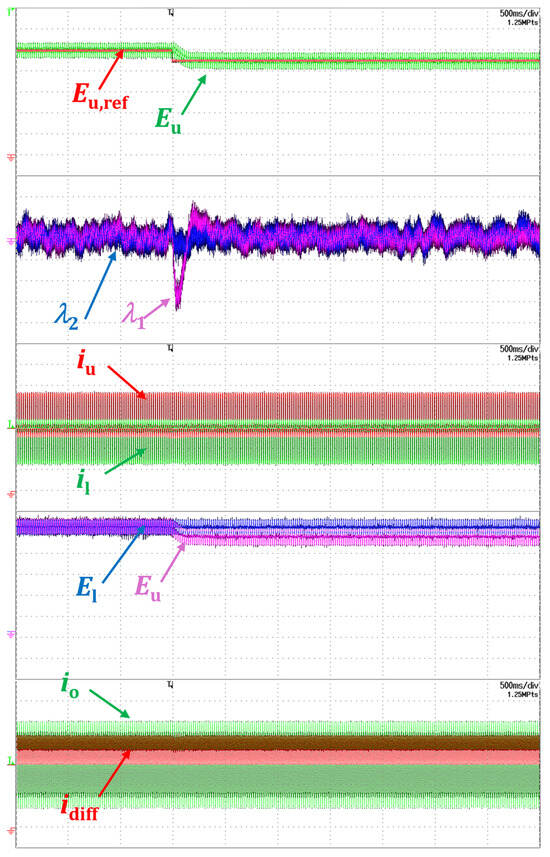
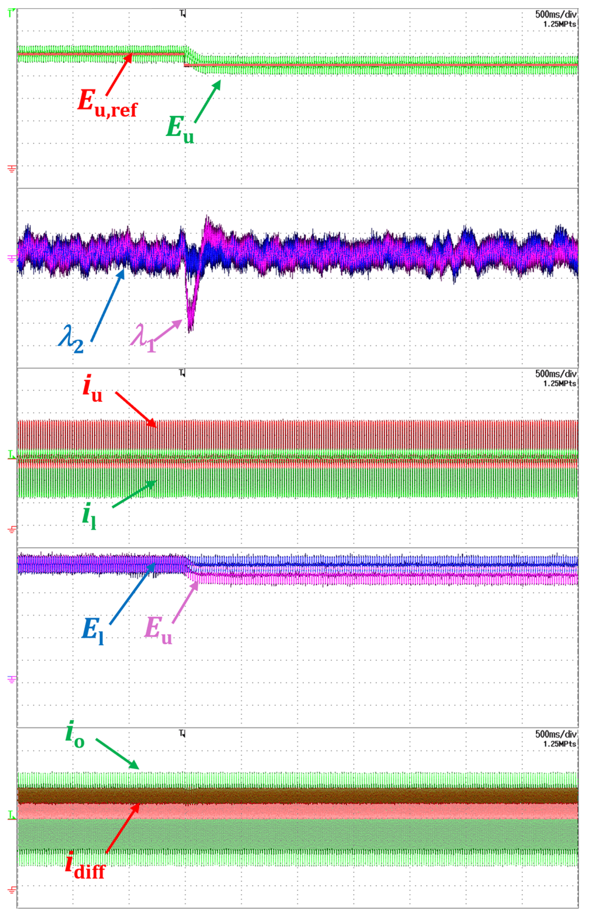
In Figure 14 the results of an experimental test conducted under the same conditions as in Figure 8 are shown. Once the system has reached a steady-state condition, a 10% decrease has been imposed to the reference value of the upper arm voltage, corresponding to a reduction from 100 V to 90 V, whereas the reference value has been maintained constant (100 V). The value of rapidly drops to track the new reference voltage, while the behavior of is unaffected. As can be seen, the actual values of and rapidly track the corresponding reference values, whereas the output current maintain the expected sinusoidal waveform. These results are very similar to those obtained with computer simulations and confirm that the proposed strategy successfully achieves decoupled control of the two arms.
Figure 14.
Converter response to a step reduction in the setpoint from top to bottom: upper arm voltage reference (20 V/div, in red); upper arm voltage (20 V/div, in purple); (0.05/div, in purple, AC coupling); (0.05/div, in blue, AC coupling); upper arm current (5 A/div, in red); lower arm current (5 A/div, in green); upper arm voltage (20 V/div, in purple); lower arm voltage (20 V/div, in blue); output current (5 A/div, in green); circulating current (5 A/div, in red).
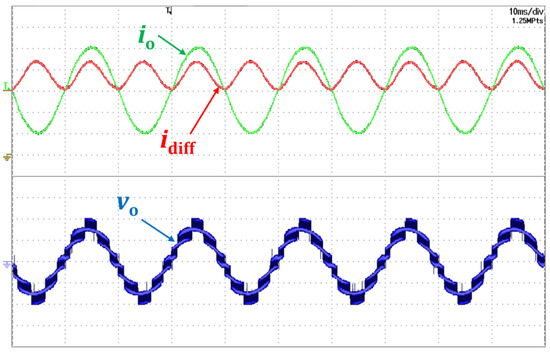
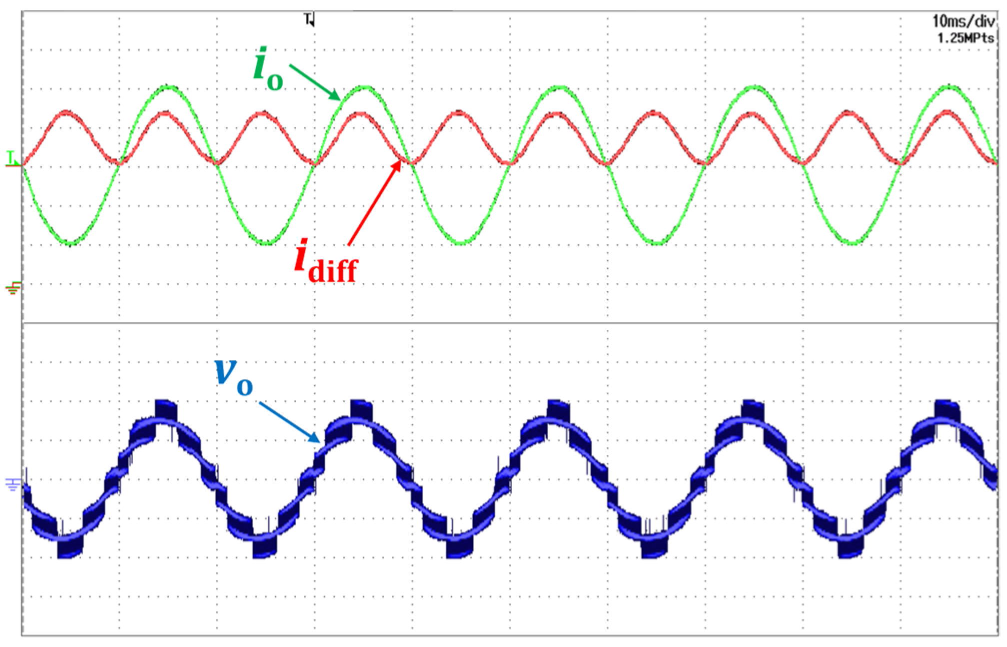
Finally, Figure 15 illustrates the steady-state waveforms of the MMC, including the output current, the circulating current and the output voltage, when the system is balanced ( and at 100% of the rated value) and the injection of the current is enabled.
Figure 15.
Converter behavior at steady-state, from top to bottom: output current (5 A/div, in green); circulating current (5 A/div, in red); output voltage (20 V/div, in blue).
The waveform of the circulating current in Figure 15 can be compared with the equivalent waveform obtained by numerical simulations in Figure 9. The peak-to-peak amplitude of the differential current is very similar (6.7 A in Figure 9, 6.9 A in Figure 15). These results confirm the consistency of simulation and experimental results and the effectiveness of the presented control scheme.
8. Conclusions
The theoretical framework proposed in this paper represents an effective alternative to that commonly used, based on the definition of the total and differential arm energies. According to the developed technique, exploiting the concept of orthogonal functions, it is possible to generate a set point for the circulating current and directly control the energy of each arm of the MMC. The experimental results, consistent with the simulation outcomes, confirm the reliability and stability of the proposed methodology. When controlled using the proposed innovative strategy, the MMC demonstrates performance comparable to that of established control methods. However, the presented theoretical framework offers a different perspective that can stimulate new ideas and suggest original approaches for the design of innovative control techniques.
This study investigates and evaluates the operational characteristics of a single-leg MMC. While the primary emphasis lies in the formulation of the leg circulating current, the proposed analytical framework is equally applicable to three-phase MMC configurations.
Author Contributions
Conceptualization, R.A.T., G.R. and L.Z.; methodology, R.A.T., L.V., G.R., M.M. and L.Z.; validation, R.A.T., A.F., L.V., G.R. and M.M.; formal analysis, R.A.T., A.F., L.V., G.R. and M.M.; investigation, R.A.T. and G.R.; writing—original draft preparation, R.A.T., M.Q.A., G.R., L.Z. and A.T.; writing—review and editing, M.Q.A., A.F., L.V., G.R., M.M., L.Z. and A.T.; supervision, L.Z. and A.T.; project administration, L.Z. and A.T. All authors have read and agreed to the published version of the manuscript.
Funding
This work was supported in part by the National Recovery and Resilience Plan (NRRP), Mission 4 Component 2 Investment 1.3- Call for tender No. 1561 of 11.10.2022 of Ministero dell’Università e della Ricerca (MUR), funded by the European Union–NextGenerationEU. Award Number: Project code PE0000021, Concession Decree No. 1561 of 11.10.2022 adopted by Ministero dell’Università e della Ricerca (MUR), CUP “J33C22002890007”. Project title “Network 4 Energy Sustainable Transition–NEST”.
Data Availability Statement
The original contributions presented in this study are included in the article. Further inquiries can be directed to the corresponding author(s).
Conflicts of Interest
The authors declare that the research was conducted in the absence of any commercial or financial relationships that could be construed as a potential conflict of interest.
References
- Marquardt, R. Stromrichterschaltungen Mit Verteilten Energiespeichern. German Patent DE 201 22 923 U1, 21 November 2001. [Google Scholar]
- Li, G.; Liang, J. Modular Multilevel Converters: Recent Applications [History]. IEEE Electrif. Mag. 2022, 10, 85–92. [Google Scholar] [CrossRef] [Scilit]
- Akagi, H. Classification, terminology, application of the modular multilevel cascade converter (MMCC). IEEE Trans. Power Electron. 2011, 26, 3119–3130. [Google Scholar] [CrossRef] [Scilit]
- Saeedifard, M.; Iravani, R. Dynamic Performance of a Modular Multilevel Back-to-Back HVDC System. IEEE Trans. Power Deliv. 2010, 25, 2903–2912. [Google Scholar] [CrossRef] [Scilit]
- Du, S.; Wu, B.; Tian, K.; Zargari, N.R.; Cheng, Z. An Active Cross-Connected Modular Multilevel Converter (AC-MMC) for a Medium-Voltage Motor Drive. IEEE Trans. Ind. Electron. 2016, 63, 4707–4717. [Google Scholar] [CrossRef] [Scilit]
- Lee, J.W.; Kim, J.W.; Lee, C.W.; Park, B.G. Common-Mode Voltage Reduction of Modular Multilevel Converter Using Adaptive High-Frequency Injection Method for Medium-Voltage Motor Drives. Energies 2024, 17, 1367. [Google Scholar] [CrossRef] [Scilit]
- Hariri, R.; Sebaaly, F.; Kanaan, H.Y. A Review on Modular Multilevel Converters in Electric Vehicles. In Proceedings of the 46th Annual Conference of the IEEE Industrial Electronics Society (IECON), Singapore, 18–21 October 2020. [Google Scholar] [CrossRef] [Scilit]
- Mei, J.; Xiao, B.; Shen, K.; Tolbert, L.M.; Zheng, J.Y. Modular multilevel inverter with new modulation method and its application to photovoltaic grid-connected generator. IEEE Trans. Power Electron. 2013, 28, 5063–5073. [Google Scholar] [CrossRef] [Scilit]
- Bakir, Y.N.; de Pablo, S.; Martinez-Rodrigo, F.; Aljawary, Z.A.; Herrero-de Lucas, L.C. Nearest Vector Control Method Applied to an MMC for PV Generation. Energies 2024, 17, 1795. [Google Scholar] [CrossRef] [Scilit]
- Lyu, J.; Cai, X.; Molinas, M. Optimal Design of Controller Parameters for Improving the Stability of MMC-HVDC for Wind Farm Integration. IEEE J. Emerg. Sel. Top. Power Electron. 2018, 6, 40–53. [Google Scholar] [CrossRef] [Scilit]
- Barresi, M.; Ferri, E.; Piegari, L. An MV-Connected Ultra-Fast Charging Station Based on MMC and Dual Active Bridge with Multiple dc Buses. Energies 2023, 16, 3960. [Google Scholar] [CrossRef] [Scilit]
- Camurca, L.; Pereira, T.; Hoffmann, F.; Liserre, M. Analysis, Limitations, and Opportunities of Modular Multilevel Converter-Based Architectures in Fast Charging Stations Infrastructures. IEEE Trans. Power Electron. 2022, 37, 10747–10760. [Google Scholar] [CrossRef] [Scilit]
- Dekka, A.; Wu, B.; Fuentes, R.L.; Perez, M.; Zargari, N.R. Evolution of Topologies, Modeling, Control Schemes, and Applications of Modular Multilevel Converters. IEEE J. Emerg. Sel. Top. Power Electron. 2017, 5, 1631–1656. [Google Scholar] [CrossRef] [Scilit]
- Perez, M.A.; Ceballos, S.; Konstantinou, G.; Pou, J.; Aguilera, R.P. Modular Multilevel Converters: Recent Achievements and Challenges. IEEE Open J. Ind. Electron. Soc. 2021, 2, 224–239. [Google Scholar] [CrossRef] [Scilit]
- Hagiwara, M.; Akagi, H. Control and Experiment of Pulse Width Modulated Modular Multilevel Converters. IEEE Trans. Power Electron. 2009, 24, 1737–1746. [Google Scholar] [CrossRef] [Scilit]
- Lizana, R.; Perez, M.A.; Arancibia, D.; Espinoza, J.R.; Rodriguez, J. Decoupled Current Model and Control of Modular Multilevel Converters. IEEE Trans. Ind. Electron. 2015, 62, 5382–5392. [Google Scholar] [CrossRef] [Scilit]
- Isik, S.; Alharbi, M.; Bhattacharya, S. An Optimized Circulating Current Control Method Based on PR and PI Controller for MMC Applications. IEEE Trans. Ind. Appl. 2021, 57, 5074–5085. [Google Scholar] [CrossRef] [Scilit]
- Yang, Q.; Saeedifard, M.; Perez, M.A. Sliding Mode Control of the Modular Multilevel Converter. IEEE Trans. Ind. Electron. 2019, 66, 887–897. [Google Scholar] [CrossRef] [Scilit]
- Yang, X.; Li, Z.; Zheng, T.Q.; You, X.; Kobrle, P. Virtual Impedance Sliding Mode Control-Based MMC Circulating Current Suppressing Strategy. IEEE Access 2019, 7, 26229–26240. [Google Scholar] [CrossRef] [Scilit]
- Perez, M.A.; Rodriguez, J.; Fuentes, E.J.; Kammerer, F. Predictive Control of AC-AC Modular Multilevel Converters. IEEE Trans. Ind. Electron. 2012, 59, 2832–2839. [Google Scholar] [CrossRef] [Scilit]
- Kadhum, H.; Watson, A.J.; Rivera, M.; Zanchetta, P.; Wheeler, P. Model Predictive Control of a Modular Multilevel Converter with Reduced Computational Burden. Energies 2024, 17, 2519. [Google Scholar] [CrossRef] [Scilit]
- Rivero, S.; Mora, A.; Correa, M.; Pereda, J. Long-Horizon MPC Reference Generator for Circulating Currents in Modular Multilevel Converter-Based Variable-Speed Drives. IEEE Trans. Ind. Electron. 2025, 72, 7785–7794. [Google Scholar] [CrossRef] [Scilit]
- Jouybary, H.S.; Mpanda Mabwe, A.; Arab Khaburi, D.; El Hajjaji, A. An LMI-Based Linear Quadratic Regulator (LQR) Control for Modular Multilevel Converters (MMCs) Considering Parameters Uncertainty. IEEE Access 2024, 12, 111888–111898. [Google Scholar] [CrossRef] [Scilit]
- She, X.; Huang, A.; Ni, X.; Burgos, R. AC circulating currents suppression in modular multilevel converter. In Proceedings of the 38th Annual Conference on IEEE Industrial Electronics Society (IECON), Montreal, QC, Canada, 25–28 October 2012. [Google Scholar] [CrossRef] [Scilit]
- Li, B.; Zhou, S.; Xu, D.; Yang, R.; Xu, D.; Buccella, C.; Cecati, C. An Improved Circulating Current Injection Method for Modular Multilevel Converters in Variable-Speed Drives. IEEE Trans. Ind. Electron. 2016, 63, 7215–7225. [Google Scholar] [CrossRef] [Scilit]
- Reddy, G.A.; Shukla, A. Arm-Current-Sensorless Circulating Current Control of MMC. IEEE Trans. Ind. Appl. 2022, 58, 444–456. [Google Scholar] [CrossRef] [Scilit]
- Pou, J.; Ceballos, S.; Konstantinou, G.; Agelidis, V.G.; Picas, R.; Zaragoza, J. Circulating Current Injection Methods Based on Instantaneous Information for the Modular Multilevel Converter. IEEE Trans. Ind. Electron. 2015, 62, 777–788. [Google Scholar] [CrossRef] [Scilit]
- Zarri, L.; Tani, A.; Mengoni, M.; Bonavoglia, M.; Serra, G.; Casadei, D.; Teodorescu, R. Control of modular multilevel converters based on time-scale analysis and orthogonal functions. In Proceedings of the 40th Annual Conference of the IEEE Industrial Electronics Society (IECON), Dallas, TX, USA, 29 October–1 November 2014. [Google Scholar] [CrossRef] [Scilit]
- Rizzoli, G.; Mengoni, M.; Mantellini, M.; Sala, G.; Zarri, L.; Tani, A.; Casadei, D. Decoupled Control of the Arms of a Modular Multilevel Converter with Orthogonal Reference Signals. In Proceedings of the 21st European Conference on Power Electronics and Applications (EPE ‘19 ECCE Europe), Genova, Italy, 3–5 September 2019. [Google Scholar] [CrossRef] [Scilit]
- Gui, Q.; Fehr, H.; Gensior, A. Energy Control of Modular Multilevel Converters for Drive Applications at Low Frequency Using General Averaging. IEEE Trans. Power Electron. 2024, 39, 5239–5256. [Google Scholar] [CrossRef] [Scilit]
- Sun, P.; Tian, Y.; Pou, J.; Konstantinou, G. Beyond the MMC: Extended Modular Multilevel Converter Topologies and Applications. IEEE Open J. Power Electron. 2022, 3, 317–333. [Google Scholar] [CrossRef] [Scilit]
- Barros, L.A.M.; Martins, A.P.; Pinto, J.G. A Comprehensive Review on Modular Multilevel Converters, Submodule Topologies, and Modulation Techniques. Energies 2022, 15, 1078. [Google Scholar] [CrossRef] [Scilit]
- Fan, B.; Wang, J.; Yu, J.; Mocevic, S.; Rong, Y.; Burgos, R.; Boroyevich, D. Cell Capacitor Voltage Switching-Cycle Balancing Control for Modular Multilevel Converters. IEEE Trans. Power Electron. 2022, 37, 2525–2530. [Google Scholar] [CrossRef] [Scilit]
- Holmes, M.H. Introduction to Perturbation Methods, 2nd ed.; Springer: London, UK, 2013. [Google Scholar] [CrossRef] [Scilit]
- Jazar, R.N. Perturbation Methods in Science and Engineering; Springer: Cham, Switzerland, 2021. [Google Scholar] [CrossRef] [Scilit]

Disclaimer/Publisher’s Note: The statements, opinions and data contained in all publications are solely those of the individual author(s) and contributor(s) and not of MDPI and/or the editor(s). MDPI and/or the editor(s) disclaim responsibility for any injury to people or property resulting from any ideas, methods, instructions or products referred to in the content. |
© 2025 by the authors. Licensee MDPI, Basel, Switzerland. This article is an open access article distributed under the terms and conditions of the Creative Commons Attribution (CC BY) license (https://creativecommons.org/licenses/by/4.0/).