Near Real-Time Photovoltaic Power Forecasting Through Recurrent Neural Network Using Timely Open-Access Data

Abstract

This paper addresses the implementation of an algorithm to compute day-ahead forecasts of photovoltaic power production with hourly updates as time progresses. Input data includes meteorological variables and real measurements of the power produced in the previous 24 h. A key aspect of the proposed methodology is that meteorological data are accessible from open sources to ensure the model’s reproducibility. Furthermore, inputs are available with a timeliness consistent with the hourly update, hence being suitable for real applications. Leveraging recent advances in the machine learning field, a Recurrent Neural Network is implemented. Different network architectures are compared to identify the best-performing one. Operatively, the model is trained and tested using six years of data referring to a real photovoltaic plant. Subsequently, to assess the flexibility of the model, the algorithm is used in near real-time to forecast the production of a different real plant. Again, inputs are obtained from an open platform that provides hourly updated values of meteorological variables in the preceding hours with adequate timeliness for preprocessing and computations to be performed by the algorithm. Both the performance on the test set and for the near real-time application confirm the ability of the algorithm to accurately predict photovoltaic generation. In particular, on the test set, a mean absolute error of 4.5% is obtained, and for the near real-time application, a value of 2.5% is reached.

1. Introduction

In the last decades, the effects of climate change have been affecting operations in many engineering fields. In this context, the reduction of greenhouse gas emissions related to human activities has a primary importance role in international political agendas. Within this framework, the energy sector is responsible for around 85% of total global CO₂ emissions, experiencing a steadily growing trend [1]. The expanding deployment of clean energy technologies of recent years is reducing three times the effect the emissions of 2019 would have been and, in line with the European directives [2], photovoltaic (PV) power generation is expected to play a pivotal role in achieving the goal of limiting the impact of the energy sector. Nevertheless, the ever-increasing introduction of PV plants within power systems poses significant challenges [1]. Precisely, the complexity that production plants and grids are encountering is shaped by the critical need to mitigate the effects of possible power imbalance introduced by the intrinsic intermittent generation of PVs. As a consequence, flexible dispatch methodologies are required to enable a proper integration of PV generation into the existing framework [3,4]. In this regard, in recent years, many research works have focused efforts on the definition of suitable control schemes to be integrated into Energy Management Systems (EMSs) aimed at optimally managing the power dispatch of polygenerative plants and Microgrids (MGs) [5,6]. This facilitates the penetration of PV by compensating for the volatility of their output with the effective operation planning of dispatchable units and deferrable loads [7]. However, even if the EMS relies on effective tools for the solution of a constrained optimization problem, whenever input with inaccurate data (PV forecast hardly ever coincides with the actual production), it outputs a solution that is not optimal. Therefore, an important research line in this field is the implementation of effective forecasting algorithms able to accurately estimate PV power production [8]. Further, typically, EMSs provide continuous updates of the dispatching programs based on the latest available measurements and inputs, such as those of PV production [9]. As a result, the availability of accurate and timely updated forecasts can significantly improve the reliability of the program updates generated by the EMS. In this context, numerous studies conducted over the past decades have investigated methods for forecasting PV power generation, with the objective of improving prediction accuracy. Nevertheless, to the best of the authors’ knowledge, the practical implementation of these forecasting models has received comparatively little attention. While a wide range of approaches, e.g., statistically based, machine learning, and hybrid algorithms, have been proposed and validated in research settings, their deployment under actual operational conditions has rarely been explored. The reason could be the fact that, to enable an effective update of PV production forecasts, the variables on which such forecasts depend, i.e., meteorological variables and/or weather forecasts, must be timely available to be input into the models/algorithms that estimate the future PV production. A review of the existing literature suggests that this crucial aspect has rarely been considered in the development of available forecasting algorithms.

In this context, in the last decades, some approaches have been proposed to address the challenge of estimating PV generation. Different forecasting models can be distinguished based on various criteria, since there is no universal classification in the literature. The methodology used to compute PV production is currently one of the key factors differentiating them [10]. The two main groups in which PV forecasting models can be split are physically based and statistical methods. Each method comes with its specific strengths and limitations. Physically based methods are mathematical representations of physical processes, grounded in the laws of physics. Their accuracy is heavily dependent on the availability and quality of input data, as well as on the simplifying assumptions required to make computations feasible [11]. Furthermore, the computational burden due to the complexity of the equations implemented has often been identified as a key limitation. Differently, statistical methods make assumptions about the possible future PV generation. Among them, for instance, Moving Average models incorporate past error terms in predictions, positing that future values are influenced by prior errors in the model’s predictions. A critical aspect of the performance of these models is the hypothesis of stationarity of the data. To address this issue, AutoRegressive Integrated Moving Average (ARIMA) models have been proposed. Nevertheless, also in this case, the computational burden may become a limiting factor, especially for short- and medium-term time horizons [12]. To overcome the identified limitations, in recent years, some research works in this field have started introducing models based on machine learning techniques with promising results [13,14]. These methods can infer relationships among inputs directly from observations. For this reason, one fundamental aspect of machine learning algorithms is the possibility of accessing reliable historical data to properly train the model. Several algorithms have been proposed in recent years to forecast PV generation. Nevertheless, the ease and the way in which input data can operatively be retrieved for practical application has hardly ever been addressed. For instance, a day-ahead PV power forecasting model for big and medium-sized plants was implemented through the application of a Long Short-Term Memory (LSTM) Recurrent Neural Network (RNN) in [15]. However, the need for more than 40 variables coming from Numerical Weather Prediction (NWP) models’ outcomes makes the near real-time application and use hard to handle. Authors of [14] compared the performance of transformer models and Convolutional Neural Networks (CNNs) to forecast the production of PV plants. However, the input data used are available every six hours, hence limiting the updates of the models depending on the latency of inputs. The authors of the study in [16] used a model consisting of combining transformers and an LSTM network to forecast the production of residential PV plants. The training data consisted of meteorological variables obtained from on-site measurements and of outputs of an NWP model. As a result, the reproducibility of the model is limited by the requirement for access to proprietary data from PV system owners and is further constrained by the dependence on forecasts produced by the NWP model. Researchers of [17] utilized an LSTM network to forecast PV power production one day ahead and up to 27 days ahead. Training and testing were performed utilizing meteorological variables retrieved from historical data, and the possibility of accessing the features needed by the network to compute the desired output for realistic applications was not addressed. In [18], a CNN-LSTM model was employed. Again, training and testing were performed on historical data, and the way these inputs can be accessed for actual applications was not described. Researchers of [19,20] conducted a performance comparison between tree-based algorithms and neural network models developed to forecast one hour ahead the power output of a PV plant using meteorological variables from previous time steps. The results indicated that RNNs achieved superior predictive performance compared with traditional neural networks and tree-based methods. In [21] a model combining Neural Prophet (NP), CNN, and an LSTM network was presented to forecast PV power production one day ahead at hourly resolution. The algorithm in [21] was implemented so that the NP model, i.e., an open-source time-series prediction package, is used to fit the trend characteristics, seasonal characteristics, and regressive terms of PV power data, and make preliminary predictions. Then, the characteristics of the NP fitted data and historical meteorological data are further extracted through a CNN to capture the dependence between adjacent hours. Subsequently, these features are fed into the LSTM RNN to extract long-term information. The proposed algorithm was tested on real plants, for which historical data are freely available at [22]. Historical data refer to power generation, wind speed, wind direction, surface temperature, relative humidity, global horizontal radiation, diffuse horizontal radiation, global tilted irradiance, diffuse tilted irradiance, and accumulated daily rainfall. The results obtained on the case study showed that the model achieved higher accuracy than the ordinary single prediction models, and the hybrid model outperformed other typical techniques. However, the practical applicability of the algorithm was not addressed, as the dataset used contains only historical data that are not updated in a timely manner.

Within this framework, this paper addresses the implementation of an effective algorithm to compute day-ahead forecasts of PV power production and its hourly update. Every hour, the algorithm receives as input meteorological data and the measurement of the plant power production in the previous 24 h. Leveraging recent advancements in the machine learning field and considering the outcomes of recent research works on the topic, an RNN is employed. Specifically, the training phase of the algorithm is developed using historical data related to a real PV plant and meteorological variables available from an open-access platform. Subsequently, the robustness of the algorithm is tested in near real-time by combining measured power production data of a different PV plant with respect to the one used to train the model with the required meteorological inputs, retrieved from open-access sources with timeliness consistent with the temporal limitations for hourly updates. Operatively, the algorithm is trained and tested using data from one PV plant of the Smart Polygeneration Microgrid (SPM) located in the University of Genoa Savona Campus [23]. Subsequently, to assess flexibility, the algorithm is used in a near real-time application to forecast the power production of a different PV plant of the SPM.

The two key aspects of the proposed algorithm are the following:

• Both input data for the training phase and for the near real-time application can be freely accessed as they come from open repositories, and this guarantees the complete reproducibility of the model. Hence, the algorithm can be trained for other PV plants and, after proper re-training, can be used to effectively forecast PV power production also on other plants. Further, this aspect makes it possible to avoid relying on forecasts of meteorological variables whose availability is limited (e.g., NWP models);
• Input data are available with a timeliness adequate to allow for hourly forecast updates. Consequently, the proposed algorithm is suitable for practical deployment, since it can be used in near real-time, for instance, to input reliable and updated power production forecasts into EMSs.

To the best of the authors’ knowledge, what sets the proposed methodology apart from existing approaches in the literature is the combination of the possibility to train the algorithm using open-access data and, at the same time, the possibility of accessing the required input data for near real-time applications with a frequency suitable for hourly forecast updates.

The paper is organized as follows: Section 2 details the methodology used to develop the algorithm. Section 3 presents the case study, and Section 4 shows the related results. Finally, Section 5 concludes the contribution.

2. Methodology

2.1. Input Data

The proposed model employs an RNN to forecast PV power generation, utilizing as inputs meteorological data, temporal indication, and PV production of previous time steps. In detail, at time step $t$, the target of the model is to predict the PV power production for the following $(t+T)$ time steps, where $T$ indicates the forecast horizon. The feature vector includes values of PV power and weather variables corresponding to the $T$ time steps preceding $t$, i.e., from time steps $(t-T)$ to $(t-1)$, together with the related temporal indication referred to the month, day, and hour. These variables, referred to as features in the machine learning field, are selected based on well-established correlations with PV power output. Specifically, the considered meteorological data are the height of the sun, the solar radiation, the temperature, and wind speed, since their influence on PV production has been largely demonstrated [24]. The samples of the target variable are retrieved from historical data of PV generation collected over several years from a real PV plant. Additionally, to account for daily periodicity and seasonal patterns typical of PV generation [25], the Seasonal-Trend decomposition combined with LOcally wEighted Scatterplot Smoothing (LOESS) (STL) is applied to all meteorological variables, resulting in the inclusion of trend, seasonal, and residual components amongst the features. The adoption of STL decomposition is motivated by its capacity to handle seasonality of any frequency and by its robustness to outliers [26,27,28,29]. Furthermore, the inclusion of the STL decomposition is supported by the findings of previous analyses presented in [19], which demonstrated that incorporating the STL decomposition of meteorological variables as inputs to the algorithm leads to better performance compared to using the meteorological variables alone. Hence, in this work, for each time step of a time series, the LOESS smoother fits a weighted polynomial regression, and the process continues until trend and seasonality stabilize. At the end of the STL process, the seasonal and trend components are extracted from the time series, and the residuals are collected in a separated component.

An introduction to the STL decomposition procedure follows.

Time series data can exhibit a variety of patterns, and it is often helpful to split them into several components, each representing an underlying pattern category [29]. STL is one of the methods for decomposing time series [26]. Assuming an additive decomposition, one can write:

$$z_t=z_t^{tr}+z_t^{se}+z_t^{re}$$

(1)

where $z_t$ is the time series data in its original form, referred to time step $t$, $z_t^{tr}$ is the trend component, $z_t^{se}$ is the seasonal component, and $z_t^{re}$ is the residual component. In detail, the trend component reflects the long-term progression of the data; the seasonal component identifies recurrent patterns that repeat over a fixed period; the residual term captures random fluctuations or irregularities in the data. The STL algorithm operates through two recursive procedures to decompose the original data into the three components: an inner loop nested inside an outer loop.

• During each iteration of the inner loop, both the seasonal and trend components are updated once. First, seasonal smoothing is applied to update the seasonal term, subsequently the trend smoothing updates the trend component. Smoothing is performed utilizing the LOESS regression, i.e., a methodology to estimate a smooth function $\hat{g}(z)$ that captures the underlying relationship between a variable $z$ and a response variable $u$, given a set of noisy observations $\left(z_i,u_i\right)$. The core idea is that, for each point $z_0$, LOESS fits a weighted least squares regression using nearby points. Therefore, points closer to $z_0$ receive higher weights, and distant points receive lower weights. To compute $\widehat{g}\left(z\right)$ a positive integer $q$, representing the bandwidth, i.e., the maximum distance for which points are included in the local regression, is first chosen. The $q$ values of $z_i$ that are closest to $z_0$ are selected, and each is given a weight ${\omega }_i(z_0)$ based on its distance from $z_0$, assigned using the tricube function. Then a polynomial of degree $d$ is fitted to the data, with ${\omega }_i(z_0)$. The estimated value at $z_0$ is $\widehat{g}(z_0)$.
• By applying this procedure to every data point, the resulting output is the smoothed curve $\widehat{g}(z)$.
• Each iteration of the outer loop includes a complete execution of the inner loop, followed by the computation of robustness weights. These weights are then utilized in the inner-loop run to lessen the impact of irregularities on the trend and seasonal components. Such weights indicate how extreme the residual term is.

2.2. Algorithm

In this work, the problem of forecasting PV production is addressed as a regression problem utilizing an RNN. The reason for the choice lies in the fact that, in this field, several research works demonstrated that RNNs show excellent short and medium-term forecasting performances [15,19,20], thus resulting in being suitable for the application presented. Precisely, since PV power forecasting is a time-series problem where future time steps depend sequentially on past time steps in a non-linear manner, RNNs are particularly well-suited to address the desired task [19,20,30]. Among RNNs, recent research works [19,20,31,32] have emphasized the effectiveness of LSTM RNNs, since their specific structure enables both short- and long-term dependencies and mitigates issues associated with vanishing gradients to be captured. Consequently, in this work, an LSTM RNN is used. To avoid making a priori assumptions on the structure of the network, the performance obtained using different architectures is compared. Several parameters defining the network structure are considered. In detail, initially, a simple LSTM RNN consisting of a single hidden layer is implemented. This configuration is often sufficient to capture relationships in simple problems. However, for more complex problems, a single layer may not be enough to fully model the correlations between inputs and outputs. Hence, subsequently, deep LSTM RNNs, i.e., RNNs with more than one layer, are developed. The adoption of multiple layers results in a more sophisticated architecture that may increase training and computational times. To assess whether performance improvements can be achieved while maintaining a comparable computational effort, the performance of RNNs with different numbers of layers is compared. Moreover, for all the networks created, the best combination of additional parameters defining the structure is sought.

A brief introduction to LSTM networks follows, further details can be found in [33,34]. From now on, bold letters indicate matrices, and non-bold letters denote scalars.

Let us consider $N_A$, representing the number of time samples in the dataset. Additionally, let us formalize the dataset as $\mathit{X}$, that is a matrix ${\mathit{M}}_{N_A\times C}(\mathbb{R})$, where $C$ is the number of features, i.e., the input variables used to forecast the desired target. Indicating with $T<N_A$ the chosen length of a time series, at each time step $t>T$, the matrix ${\mathit{x}}_t\in {\mathit{M}}_{T\times C}(\mathbb{R})$ is obtained by extracting from $\mathit{X}$ the rows from $t-T$ to $t-1$ and all the associated $C$ columns. At time step $t$, the objective of the problem is to predict the PV power production for the next $T$ time steps, i.e., to generate an output sample ${\mathit{y}}_t\in {\mathbb{R}}^T$. From a machine learning point of view, it is a spatiotemporal forecasting regression problem where, at time step $t$, the aim is to predict the most likely ${\widehat{\mathit{y}}}_t\in {\mathbb{R}}^T$, given previous observations:

$${\widehat{\mathit{y}}}_t=\underset{{\mathit{y}}_t}{\mathrm{argmax}} P\left({\mathit{y}}_t|{\mathit{x}}_t\right)$$

(2)

where $P({\mathit{y}}_t|{\mathit{x}}_t)$ represents the conditioned probability of ${\mathit{y}}_t$ given ${\mathit{x}}_t$, and $\underset{{\mathit{y}}_t}{\mathrm{argmax}}\left(∎\right)$ indicates the maximization of its argument $\left(∎\right)$ in the variable ${\mathit{y}}_t$. It should be noted that ${\mathit{x}}_t$ includes, amongst the features, the values referred to the involved meteorological variables, the temporal indication referred to the month, day, and hour, and the measure of the target variable at $t-T,\dots ,t-1$. In principle, RNNs with enough hidden units can remember inputs from long in the past. However, in practice, the vanishing gradient problem may arise, limiting the ability to capture long-term dependencies. Consequently, the possibility of regulating the flow of information through the network, allowing retaining relevant information for extended time spans, and the possibility of learning when to update the hidden state, could be useful to map relationships for which only a portion of the sequence may influence future estimates. This feature can be used to selectively remember important pieces of information when they are first seen or to learn when to forget information that no longer has an influence on the outputs. The selection of information is performed due to a gating unit that simultaneously controls the forgetting factor and the decision to update the state unit. The resulting architecture is referred to as a gated RNN, whose units are also known as gated recurrent units [33]. Among gated RNNs, LSTMs are networks in which self-loops to produce paths where the gradient can flow for long durations are introduced. By making the weight of this self-loop gated (controlled by another hidden unit), the time scale of integration can be changed dynamically. Referring to time step $t$, this is performed by augmenting the hidden state ${\mathit{h}}_t$ of a traditional RNN with a memory cell. Three gates are needed to control this cell: the output gate ${\mathit{o}}_t$, which determines what is read out, the input gate ${\mathit{i}}_t$, which determines what is read in, and the forget gate ${\mathit{f}}_t$, which determines when the cell should be reset. The actual update to the candidate cell is either the candidate cell (if the input gate is on) or the old cell (if the not-forget gate is on). Finally, the hidden state is computed as a transformed version of the cell, provided the output gate is on. (3)–(7) show the related equations [34]:

$${\mathit{f}}_t=\sigma \left({\mathit{W}}_{xf}{\mathit{x}}_t+{\mathit{W}}_{hf}{\mathit{h}}_{t-1}+{\mathit{b}}_f\right)$$

(3)

$${\mathit{i}}_t=\sigma \left({\mathit{W}}_{xi}{\mathit{x}}_t+{\mathit{W}}_{hi}{\mathit{h}}_{t-1}+{\mathit{b}}_i\right)$$

(4)

$${\mathit{o}}_t=\sigma \left({\mathit{W}}_{xo}{\mathit{x}}_t+{\mathit{W}}_{ho}{\mathit{h}}_{t-1}+{\mathit{b}}_o\right)$$

(5)

$${\mathit{c}}_t={\mathit{f}}_t\circ {\mathit{c}}_{t-1}+{\mathit{i}}_t\circ tanh\left({\mathit{W}}_{xc}{\mathit{x}}_t+{\mathit{W}}_{hc}{\mathit{h}}_{t-1}+{\mathit{b}}_c\right)$$

(6)

$${\mathit{h}}_t={\mathit{o}}_t\circ tanh\left({\mathit{c}}_t\right)$$

(7)

In (3)–(6), ${\mathit{W}}_{xf},{\mathit{W}}_{xi},{\mathit{W}}_{xo},{\mathit{W}}_{xc}$ denote, respectively, the weight matrix ${\mathit{M}}_{F\times C}(\mathbb{R})$, associated with the forget gate, input gate, output gate and the cell candidate, and $F$ indicates the dimension of the hidden state. Differently, in (3)–(6) ${\mathit{W}}_{hf},{\mathit{W}}_{hi},{\mathit{W}}_{ho},{\mathit{W}}_{hc}$ indicate the recurrent weight matrix ${\mathit{M}}_{F\times F}(\mathbb{R})$, respectively, associated with the forget gate, input gate, output gate, and with the cell candidate. Finally, in (3)–(6), the bias vectors used, respectively, for the forget gate, input gate, output gate, and for the cell candidate, are indicated with ${\mathit{b}}_f,{\mathit{b}}_i,{\mathit{b}}_o,{\mathit{b}}_c\in {\mathbb{R}}^F$. The sigmoid function $\sigma \left(z\right)=1/(1+e^{-z})$ and the hyperbolic tangent are used as activation functions in the various gates; when written with vector arguments, they are meant to be evaluated element by element. Operator $\circ$ denotes the Hadamard product, i.e., the element-wise multiplication.

In a deep LSTM network, multiple hidden layers form the network structure. Referring to the general formulation for calculating the hidden state (7), and considering the stacking of multiple hidden layers, identified by the index $l=1,\dots ,L$, the hidden state of the $l^{th}$ layer at time step $t$ is ${\mathit{h}}_t^l\in {\mathbb{R}}^F$ and is computed by (8):

$${\mathit{h}}_t^l={\mathit{o}}_t^l\circ tanh\left({\mathit{c}}_t^l\right)$$

(8)

where ${\mathit{c}}_t^l\in {\mathbb{R}}^F$ and ${\mathit{o}}_t^l\in {\mathbb{R}}^F$ are the candidate cell and the output of the $l^{th}$ layer. In regression problems, the output of the neural network is typically obtained by applying a linear transformation to the outputs of the last hidden layer in the output layer. Hence, the final estimate for time step $t$ can be computed as (9):

$${\widehat{\mathit{y}}}_t={\mathit{W}}_{ho}^L{\mathit{h}}_t^L+{\mathit{b}}_o^L$$

(9)

In (9) ${\widehat{\mathit{y}}}_t$ represents the estimate produced by the network for time step $t$, while ${\mathit{W}}_{ho}^L$ and ${\mathit{b}}_o^L\in {\mathbb{R}}^T$ denotes the weight matrix ${\mathit{M}}_{T\times F}(\mathbb{R})$ and the bias vector of the $L^{th}$ output layer, respectively.

Together with the number of layers, additional parameters defining the structure of the network are considered in the implemented methodology. Precisely, the best combination of the number of neurons, the batch size, the number of epochs, and the learning rate is searched for [34]. More in detail, the number of neurons determines the model’s capacity to learn complex patterns from the input sequences. Increasing the number of neurons can enhance the capacity of the model to learn complex patterns, but can also raise the risk of overfitting if not properly regularized. Differently, the batch size, defined as the number of samples processed before parameters are updated, and the number of epochs, which defines the number of times the algorithm will work through the entire training dataset, can influence convergence and generalization capability. Finally, the learning rate controls how much the model changes in response to the estimated error each time the weights are updated and can influence convergence and stability of the model.

To identify the best-performing network architecture, performance obtained using combinations of the aforementioned parameters is compared. The optimal set of such parameters is sought using a grid search approach, which systematically explores different combinations [34].

Operatively, the implementation of the algorithm consists of two phases. In detail, initially, the training phase of the algorithm is implemented utilizing a portion of the available data in $\mathit{X}$, collected in the so-referred training set. Subsequently, the remaining portion of the data is collected in the so-called test set and is used to evaluate the model’s performance. To assess the performance, the estimates computed by the RNN for the samples in the test set are compared with the real target values. The evaluation metrics used are those commonly employed in regression tasks, i.e., the Mean Absolute Error (MAE), the Root Mean Square Error (RMSE), and the coefficient of determination ($R^2$). Specifically, for a test set composed of $n$ samples, the MAE, RMSE, and $R^2$ can be computed as shown in (10)–(12).

$$MAE={\displaystyle \frac{1}{n}}\sum _{i=1}^n\left|{\widehat{\mathit{y}}}_i-{\mathit{y}}_i\right|$$

(10)

$$RMSE=\sqrt{{\displaystyle \frac{1}{n}}\sum _{i=1}^n{\left({\widehat{\mathit{y}}}_i-{\mathit{y}}_i\right)}^2}$$

(11)

$$R^2=1-{\displaystyle \frac{\sum _{i=1}^n{\left({\widehat{\mathit{y}}}_i-{\mathit{y}}_i\right)}^2}{\sum _{i=1}^n{\left({\widehat{\mathit{y}}}_i-\overline{\mathit{y}}\right)}^2}}$$

(12)

In (10)–(12) ${\mathit{y}}_i$ is the actual target value of the $i$-th test sample, ${\widehat{\mathit{y}}}_i$ is the estimated value and $\overline{\mathit{y}}$ is the mean of the actual data.

As anticipated, this work also includes a near real-time application of the algorithm. Hence, the metrics in (10)–(12) are also used to evaluate the near real-time performance of the model.

3. Case Study

3.1. Input Data

The dataset ($\mathit{X}$) created to train and test the algorithm includes PV and meteorological data related to 2015–2020, together with the related temporal indication (month, day, and hour). These latter variables are respectively indicated with ${\mathit{m}}_t,{\mathit{d}}_t,{\mathit{k}}_t$.

PV data are retrieved from the 81 kW_p PV plant of the SPM. PV power production data [W] come with a 5 min resolution. Regarding meteorological data, the repository used is the Photovoltaic Geographical Information System on the Joint Research Centre (JRC) website (PVGIS©) (https://re.jrc.ec.europa.eu/pvg_tools/en/, accessed on 24 March 2025), in which data are available at a spatial resolution of ~5 km and a temporal resolution of 1 h. The downloaded data from PVGIS are the solar radiation [W/m²], indicated with the variable ${\mathit{s}}_t$, the height of the sun [°], represented by the variable ${\mathit{b}}_t$, the temperature at 2 m ASL [°C], designated by the variable ${\mathit{z}}_t$, and wind speed at 10 m ASL [m/s], denoted by the variable ${\mathit{e}}_t$. PV data are re-sampled at the hourly level to match the resolution of weather data, and the related variable is ${\mathit{p}}_t$. Additionally, these data are merged with the related STL components, computed as in [26], hence the dataset $\mathit{X}$ also includes the STL components of each meteorological variable, allowing for the consideration of daily and seasonal variations in wind speed and temperature trends characteristic of the studied region, as well as the seasonal cycles of solar radiation. The trend component of the variable referred to the solar radiation, the height of the sun, the temperature, and the wind speed are represented, respectively, by ${\mathit{s}}_t^{tr}$,${\mathit{b}}_t^{tr},{\mathit{z}}_t^{tr},{\mathit{e}}_t^{tr}$. The seasonal component of the variable referred to solar radiation, the height of the sun, the temperature, and the wind speed are denoted, respectively, by ${\mathit{s}}_t^{se}$,${\mathit{b}}_t^{se},{\mathit{z}}_t^{se},{\mathit{e}}_t^{se}$. The residual component of the variable referred to solar radiation, the height of the sun, the temperature, and the wind speed are indicated, respectively, with ${\mathit{s}}_t^{re}$,${\mathit{b}}_t^{re},{\mathit{z}}_t^{re},{\mathit{e}}_t^{re}$. The resulting dataset $\mathit{X}$ is composed of $N_A$ = 52,560 h (samples), and the number of features for each sample is $C$ = 20. The feature vector for each time step $t$ is structured so that it contains the values of inputs relating to the previous $(t-T)$ time steps, with $T=24$. The algorithm outputs a time series of the PV production forecasts referring to $\left(t+1\right),\dots ,(t+T)$, collected in ${\mathit{p}}_{t+1,\dots ,t+24}$. A graphic explanation of the structure of the feature vector and of the output is provided in Figure 1, where $t$ represents the hour under consideration. The features and the target of the model are collected in Table 1.

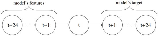
Figure 1. Temporal structure of the feature vector and of the output computed by the algorithm.

Table 1. Features and targets of the model, collected in the dataset $\mathit{X}$. The time step index appears as a subscript on each variable.

$\mathbf{Dataset}\mathit{X}$
	Variable Description	Variable
Target	PV power production	${\mathit{p}}_{t+1,\dots ,t+24}$
Features	PV power production	${\mathit{p}}_{t-24,\dots ,t-1}$
	Solar radiation	${\mathit{s}}_{t-24,\dots ,t-1}$
	Height of the sun	${\mathit{b}}_{t-24,\dots ,t-1}$
	Temperature	${\mathit{z}}_{t-24,\dots ,t-1}$
	Wind speed	${\mathit{e}}_{t-24,\dots ,t-1}$
	Month	${\mathit{m}}_{t-24,\dots ,t-1}$
	Day	${\mathit{d}}_{t-24,\dots ,t-1}$
	Hour	${\mathit{k}}_{t-24,\dots ,t-1}$
	Solar radiation trend component	${\mathit{s}}_{t-24,\dots t-1}^{tr}$
	Height of the sun trend component	${\mathit{b}}_{t-24,\dots t-1}^{tr}$
	Temperature trend component	${\mathit{z}}_{t-24,\dots t-1}^{tr}$
	Wind speed trend component	${\mathit{e}}_{t-24,\dots t-1}^{tr}$
	Solar radiation seasonal component	${\mathit{s}}_{t-24,\dots t-1}^{se}$
	Height of the sun seasonal component	${\mathit{b}}_{t-24,\dots t-1}^{se}$
	Temperature seasonal component	${\mathit{z}}_{t-24,\dots t-1}^{se}$
	Wind speed seasonal component	${\mathit{e}}_{t-24,\dots t-1}^{se}$
	Solar radiation residual component	${\mathit{s}}_{t-24,\dots t-1}^{re}$
	Height of the sun residual component	${\mathit{b}}_{t-24,\dots t-1}^{re}$
	Temperature residual component	${\mathit{z}}_{t-24,\dots t-1}^{re}$
	Wind speed residual component	${\mathit{e}}_{t-24,\dots t-1}^{re}$

As anticipated, after evaluating the model’s forecasting capability on historical data, the near real-time operational performance is assessed. The selected PV plant is located again in the SPM and has a power production of 21 kW_p. For this near real-time test, meteorological data are retrieved from the open-access platform Open-Meteo (https://open-meteo.com/, accessed on 1 December 2024). Open-Meteo data are updated every hour, ensuring the latest changes in conditions are captured. The available data are obtained due to measurements from various sources such as airplanes, buoys, radar systems, and satellites, and refer to air temperature [°C], wind speed [m/s], and solar radiation [W/m²]. Data come with a spatial resolution of 2.5 km and a temporal resolution of one hour. These data are made available in less than 30 min, allowing enough time for their retrieval and processing, and enabling the algorithm to generate 24-h PV production forecasts using the latest available measurements. In addition, the solar elevation angle [°] is computed using the PVlib library (https://pvlib-python.readthedocs.io/en/stable/, accessed on 1 December 2024). The actual PV power production data are retrieved from measurements of the PV plant inverter, which records measurements every 5 min. These values are averaged over each hour to match the hourly resolution of the meteorological variables.

3.2. Model Selection

The parameters considered to compare the performances of RNN with different architectures are summarized in Table 2. More in detail, as far as the number of layers, the batch size, and the number of neurons are concerned, the considered values are chosen because of previous analyses, reported in [20]. Furthermore, regarding the number of epochs, it should be noted that low values (typically fewer than 50) may result in underfitting, whereas an excessively high number (typically greater than 500) may increase the risk of overfitting [34]. To prevent this issue, an early stopping mechanism is employed. This approach halts training when no improvement in the validation loss is observed after a predetermined number of epochs, effectively reducing unnecessary computations and mitigating overfitting. Finally, the learning rate is set to 0.01 because of previous analyses addressing the topic (not reported for brevity and exposed in [20]). Dropout is also used, since in an LSTM network helps prevent overfitting by randomly disabling a portion of neurons during training, encouraging the model to develop more robust and generalizable features [33].

Table 2. Sets of the parameters considered to seek the best-performing RNN architecture.

Parameter	Values
Layers	1, 2, 3, 4
Batch Size	256, 512
Neurons	100, 150, 200
Epochs	100, 150, 200, 500
Learning Rate	0.01

The training, validation, and test sets for each generated RNN are produced by extracting, respectively, 64%, 16%, and 20% of the available (consecutive) days, respectively.

Since the core idea of this work is to ensure the reproducibility of the implemented models, the code related to the implementation of the different neural network architectures is publicly available on GitHub (https://github.com/alicelafata, accessed on 19 October 2025).

4. Results

4.1. Algorithm Performance on the Test Set

Initially, the performance of the LSTM networks is evaluated on the test set. Accordingly, Table 3 reports the MAE, RMSE, and coefficient of determination achieved by the best-performing models on the test set, categorized by the number of layers.

Table 3. MAE, RMSE, and $R^2$ on the test set obtained for the best-performing models. The parameters defining the RNN architecture are specified in the related column.

RNN	$\mathit{M}\mathit{A}\mathit{E}$ [kW]	$\mathit{R}\mathit{M}\mathit{S}\mathit{E}$ [kW]	${\mathit{R}}^2$	Neurons	Batch Size	Epochs
1-layer LSTM	3.83	6.99	0.85	200	512	<100
2-layer LSTM	3.63	7.17	0.85	150	512	<100
3-layer LSTM	3.68	7.12	0.86	100	512	<100
4-layer LSTM	3.71	7.10	0.85	200	512	<100

All training phases stopped before reaching 100 epochs. This indicates that the loss function stabilizes in fewer than 100 iterations, highlighting the model’s ability to quickly learn and capture the interactions between different data features, without the need for excessive training that could lead to overfitting. Furthermore, it is worth noting that the number of epochs required for each model decreases as the model’s structure becomes more complex. For instance, all the 1-layer LSTM models stopped training between 70 to 90 epochs, while the more complex 4-layer LSTM models halted the training process around 50 epochs. This observation is consistent with the analysis in Section 2, stating that more complex models tend to learn faster. Table 3 also highlights that the 3-layer LSTM model provides the highest $R^2$ value, along with one of the lowest RMSE and MAE values. This configuration resulted in an RMSE of 7.12 kW, and an $R^2$ coefficient of 0.86 when 100 neurons are used and the batch size is set to 512. The MAE is 3.68 kW, corresponding to ~4.5%.

As far as the RNN architecture is concerned, all the networks in Table 3 achieved their best performance with a batch size of 512. Since such a dimension for the batch size allows to include a wider variety of samples from the dataset with respect to the ones included when a batch size of 256 is considered, this outcome indicates that a batch size of 512 helps the model generalize better the addressed problem and reduces the risk of overfitting to specific patterns present in smaller batches. Moreover, in Table 3, it is shown that the 1-layer network required a higher number of neurons (200) to capture the complexity of the problem with respect to the 2- and 3-layer networks. This outcome indicates that adding more layers allows the model to learn more distributed and hierarchical representations, hence the number of neurons needed per layer to attain a satisfactory representation can be reduced. However, deeper models drive to more complex architectures, with an increased number of parameters to be learnt and optimized. This is because each additional layer processes transformed versions of the input, and if these transformations are too constrained (because of too few neurons), the network may underfit even with increased depth. This could be the reason why the network with four layers may benefit from having 200 neurons to compensate for the architectural depth.

Figure 2 shows an example of the outcomes obtained by the best-performing algorithm. Precisely, the difference between the forecasts produced by the RNN and the real measured values referred to 9 May 2020 is shown. Focusing on $t=12$ (red bar), it is possible to observe the difference ${(\mathsf{\Delta }}_t={\widehat{y}}_t-y_t)$. As the prediction time approaches the target interval, the difference between the forecasted value for $t=12$ and the measured one decreases. Specifically, as depicted in the upper panel of Figure 2, the prediction made at 09 A.M. referring to the interval between $t=10$ A.M. on 9 May and $t=09$ A.M. on the following day, results in an error of 8.78 kw. As shown in the second row of Figure 2, the forecast made at 10 A.M., covering the interval from $t=11$ A.M. on 9 May to $t=10$ A.M. on 10 May, yields an error of 6.9 kw. Finally, the prediction made at the following hour, in the lowest panel of Figure 2, shows an error of 4.24 kw. These results show that, as the forecasted time approaches, the predictions become increasingly accurate.

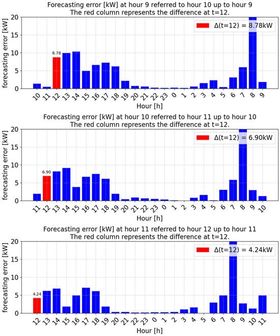
Figure 2. Difference between forecasted and observed PV power production on 9 May 2020.

Conclusively, it can be assessed that the results obtained demonstrate that having access to hourly updated data (of the PV production and of meteorological variables) enables continuous updates of PV production forecasts, significantly reducing prediction errors as the target time approaches. This is one of the key findings of this work, which, as previously highlighted, aims to show that to enable such updates, and thus improve forecast accuracy, it is essential to have timely access to data that are readily available.

As far as the computational time is concerned, the training time for each network architecture is approximately 10 h, using a medium-performance computer equipped with an Intel^® Iris^® Xe Graphics integrated GPU.

4.2. Algorithm Performance in near Real-Time

The assessment of the near real-time performance of the algorithm is conducted from December 2024 to April 2025. The RNNs utilized are the ones resulting in the best performance on the test set, presented in Table 3. The related outcomes are reported in Table 4. Results show that, with the exception of the 1-layer LSTM model, all architectures exhibit comparable performance. The RMSE values for the 2-3-4-layer LSTM models are below 5%, indicating a satisfactory generalization capability of the RNN when applied to a different PV installation with respect to the one used for the training phase. Among the evaluated models, the 3-layer LSTM achieved the best performance, reaching an RMSE of 1.13 kw, and an $R^2$ of 0.86. The MAE is 0.53 kw, corresponding to ~2.5%.

Table 4. MAE, RMSE, and $R^2$ for the near real-time application of the algorithms.

RNN	$\mathit{M}\mathit{A}\mathit{E}$ [kW]	$\mathit{R}\mathit{M}\mathit{S}\mathit{E}$ [kw]	${\mathit{R}}^2$
1-layer LSTM	1.11	1.58	0.74
2-layer LSTM	0.55	1.13	0.85
3-layer LSTM	0.53	1.13	0.86
4-layer LSTM	0.58	1.19	0.85

Figure 3 presents an example extracted from the control system of the SPM, in which the real-time acquisition of the forecasts computed by the RNN is visible. Panel (a) shows real measurements with a 5 min resolution on 1 April, and Panel (b) displays the same data aggregated on an hourly basis. In the lower panels, Panel (c) shows the forecasts acquired at 10:00 A.M., and Panel (d) shows the forecasts acquired at 11:00 A.M. The prediction error at 10:00 A.M. is ${\mathsf{\Delta }}_t=$ 1.27 kw. The error of the forecast acquired at 10:00 A.M. (computed at 09:00 A.M.), referred to 11:00 A.M., is 2.57 kw. The forecast acquired at 11:00 A.M. (computed at 10:00 A.M.), referred to 11:00 A.M., has an error of 1.85 kw. Once again, it becomes evident that the closer the forecasted time is, the smaller the prediction error becomes.

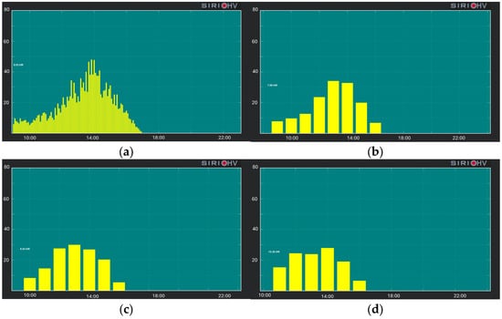
Figure 3. Near real-time PV production acquired by the SPM control system (a), hourly aggregated production (b), acquisition of the forecasts at h. 10:00 A.M. (c), acquisition of the forecasts at h. 11:00 A.M. (d).

It is important to highlight that these results are made possible by the ability to download updated meteorological measurements on an hourly basis, thus avoiding the need to rely on outdated forecasts made well in advance of the target time. Precisely, the time required to download meteorological data, receive measurements of the PV plant inverter, and process them so that they can be used as input for the model is, on average across the time samples considered, 58.4 s. Subsequently, the model itself takes an average of 2.8 s to provide predictions.

The results obtained for the near real-time application of the algorithm further confirm that the proposed methodology is capable of providing accurate estimates of PV plant production based on the considered meteorological data. Moreover, the low values of the MAE and RMSE demonstrate that the possibility to actually access hourly updated meteorological variables enables the neural network to update its forecasts, thereby improving overall accuracy. This aspect represents the second key finding of this research work, since near real-time application is made possible due to the chance to retrieve input data with adequate timeliness, and given that the corresponding results proved to be accurate. Further, the fact that data to be input into the RNN to produce accurate estimates are freely accessible avoids the need to rely on meteorological data from complex weather prediction models or other sources that are often difficult to access or unsuitable for practical, real-world applications.

5. Conclusions

This paper presented an hourly-updating forecasting model based on a Recurrent Neural Network to forecast photovoltaic power production, utilizing open-access data. Input data refer to meteorological variables, the related temporal indication, and the measured power production in the preceding 24 h. Additionally, to address seasonal and daily variations of photovoltaic generation, seasonal trend decomposition was applied to the meteorological data; hence, the values referring to the seasonal, trend, and residual components of these variables are included amongst the features. Different network architectures were implemented to compare the related performance. Operatively, the models were trained with data referring to a real photovoltaic plant and with meteorological data downloaded from an open-access platform.

The best-performing architecture was identified as the 3-layer network, with 100 neurons and a batch size of 512. On the test set, this model achieved a mean absolute error of 3.68 kw (~4.5%). Furthermore, to assess the robustness of the model, the network architectures resulting in the best performance on the test set were used in near real-time to forecast the power production of a different photovoltaic plant. In this case, meteorological data were downloaded from an open platform providing hourly updates of the input data required, available with consistent timeliness. The 3-layer network drove to the most accurate results, with a mean absolute error of 0.53 kw (~2.5%). Both outcomes on the test set and for the near real-time application suggested the effectiveness of the proposed approach in delivering precise predictions of photovoltaic generation based on open-source data. Additionally, the results highlighted the importance of having timely, hourly meteorological updates, which enable the neural network to refine its predictions dynamically and enhance overall forecasting precision. These aspects constitute the major contributions of this research.

Based on the results obtained, possible future developments of the implemented methodology could involve the exploration of additional meteorological variables that may influence photovoltaic production, provided that such data are available from open-access sources with a temporal update suitable to allow the neural network to update the forecasts computed. Furthermore, transfer learning techniques could be investigated to enable a model trained on a specific plant, for which historical production measurements are available, to be effectively applied to other installations, without the need for retraining on each specific plant.

References

- IEA World Energy Outlook 2024. Available online: https://www.iea.org/reports/world-energy-outlook-2024 (accessed on 24 March 2025).
- European Commission Directive (EU). 2023/2413 of the European Parliament and of the Council of 18 October 2023 Amending Directive (EU) 2018/2001, Regulation (EU) 2018/1999 and Directive 98/70/EC as Regards the Promotion of Energy from Renewable Sources, and Repealing Council Directive (EU) 2015/652 2023. Available online: https://eur-lex.europa.eu/eli/dir/2023/2413/oj/eng (accessed on 24 March 2025).
- Al-Dahidi, S.; Madhiarasan, M.; Al-Ghussain, L.; Abubaker, A.M.; Ahmad, A.D.; Alrbai, M.; Aghaei, M.; Alahmer, H.; Alahmer, A.; Baraldi, P. Forecasting Solar Photovoltaic Power Production: A Comprehensive Review and Innovative Data-Driven Modeling Framework. Energies 2024, 17, 4145. [Google Scholar] [CrossRef]
- Tahir, M.F.; Yousaf, M.Z.; Tzes, A.; El Moursi, M.S.; El-Fouly, T.H. Enhanced Solar Photovoltaic Power Prediction Using Diverse Machine Learning Algorithms with Hyperparameter Optimization. Renew. Sustain. Energy Rev. 2024, 200, 114581. [Google Scholar] [CrossRef]
- Fusco, A.; Gioffrè, D.; Castelli, A.F.; Bovo, C.; Martelli, E. A Multi-Stage Stochastic Programming Model for the Unit Commitment of Conventional and Virtual Power Plants Bidding in the Day-Ahead and Ancillary Services Markets. Appl. Energy 2023, 336, 120739. [Google Scholar] [CrossRef]
- Rosini, A.; Minetti, M.; Denegri, G.B.; Invernizzi, M. Reactive Power Sharing Analysis in Islanded AC Microgrids. In Proceedings of the 2019 IEEE International Conference on Environment and Electrical Engineering and 2019 IEEE Industrial and Commercial Power Systems Europe (EEEIC/I&CPS Europe), Genova, Italy, 11–14 June 2019; pp. 1–6. [Google Scholar]
- Moretti, L.; Martelli, E.; Manzolini, G. An Efficient Robust Optimization Model for the Unit Commitment and Dispatch of Multi-Energy Systems and Microgrids. Appl. Energy 2020, 261, 113859. [Google Scholar] [CrossRef]
- Eyimaya, S.E.; Altin, N. Review of Energy Management Systems in Microgrids. Appl. Sci. 2024, 14, 1249. [Google Scholar] [CrossRef]
- Moazzen, F.; Hossain, M. A Two-Layer Strategy for Sustainable Energy Management of Microgrid Clusters with Embedded Energy Storage System and Demand-Side Flexibility Provision. Appl. Energy 2025, 377, 124659. [Google Scholar] [CrossRef]
- Hategan, S.-M.; Stefu, N.; Petreus, D.; Szilagyi, E.; Patarau, T.; Paulescu, M. Short-Term Forecasting of PV Power Based on Aggregated Machine Learning and Sky Imagery Approaches. Energy 2025, 316, 134595. [Google Scholar] [CrossRef]
- Pereira, S.; Canhoto, P.; Oozeki, T.; Salgado, R. Comprehensive Approach to Photovoltaic Power Forecasting Using Numerical Weather Prediction Data and Physics-Based Models and Data-Driven Techniques. Renew. Energy 2025, 251, 123495. [Google Scholar] [CrossRef]
- Sapundzhi, F.; Chikalov, A.; Georgiev, S.; Georgiev, I. Predictive Modeling of Photovoltaic Energy Yield Using an ARIMA Approach. Appl. Sci. 2024, 14, 11192. [Google Scholar] [CrossRef]
- Li, P.; Luo, Y.; Xia, X.; Shi, W.; Zheng, J.; Liao, Z.; Gao, X.; Chang, R. Advancing Photovoltaic Panel Temperature Forecasting: A Comparative Study of Numerical Simulation and Machine Learning in Two Types of PV Power Plant. Renew. Energy 2024, 237, 121602. [Google Scholar] [CrossRef]
- Kothona, D.; Spyropoulos, K.; Valelis, C.; Koutsis, C.; Chatzisavvas, K.C.; Christoforidis, G.C. Deep Learning Forecasting Tool Facilitating the Participation of Photovoltaic Systems into Day-Ahead and Intra-Day Electricity Markets. Sustain. Energy Grids Netw. 2023, 36, 101149. [Google Scholar] [CrossRef]
- Aslam, M.; Lee, S.-J.; Khang, S.-H.; Hong, S. Two-Stage Attention over LSTM with Bayesian Optimization for Day-Ahead Solar Power Forecasting. IEEE Access 2021, 9, 107387–107398. [Google Scholar] [CrossRef]
- Hu, Z.; Gao, Y.; Ji, S.; Mae, M.; Imaizumi, T. Improved Multistep Ahead Photovoltaic Power Prediction Model Based on LSTM and Self-Attention with Weather Forecast Data. Appl. Energy 2024, 359, 122709. [Google Scholar] [CrossRef]
- Zhai, C.; He, X.; Cao, Z.; Abdou-Tankari, M.; Wang, Y.; Zhang, M. Photovoltaic Power Forecasting Based on VMD-SSA-Transformer: Multidimensional Analysis of Dataset Length, Weather Mutation and Forecast Accuracy. Energy 2025, 324, 135971. [Google Scholar] [CrossRef]
- Gao, X.; Zang, Y.; Ma, Q.; Liu, M.; Cui, Y.; Dang, D. A Physics-Constrained Deep Learning Framework Enhanced with Signal Decomposition for Accurate Short-Term Photovoltaic Power Generation Forecasting. Energy 2025, 326, 136220. [Google Scholar] [CrossRef]
- Amin, M.A.; La Fata, A.; Procopio, R.; Invernizzi, M.; Petronijevic, M.; Mitic, I.R. Photovoltaic Power Nowcasting Using Decision-Trees Based Algorithms and Neural Networks. In Proceedings of the 2024 11th International Conference on Electrical, Electronic and Computing Engineering (IcETRAN), Nis, Serbia, 3–6 June 2024; pp. 1–6. [Google Scholar]
- La Fata, A.; Amin, M.A.; Invernizzi, M.; Procopio, R. Structurally Tuned LSTM Networks to Nowcast Photovoltaic Power Production. In Proceedings of the 2024 IEEE International Conference on Environment and Electrical Engineering and 2024 IEEE Industrial and Commercial Power Systems Europe (EEEIC/I&CPS Europe), Rome, Italy, 17–20 June 2024; pp. 1–6. [Google Scholar]
- Xiao, Z.; Huang, X.; Liu, J.; Li, C.; Tai, Y. A Novel Method Based on Time Series Ensemble Model for Hourly Photovoltaic Power Prediction. Energy 2023, 276, 127542. [Google Scholar] [CrossRef]
- DKA Solar Centre. Available online: https://dkasolarcentre.com.au/download?location=alice-springs (accessed on 21 November 2025).
- Bonfiglio, A.; Delfino, F.; Pampararo, F.; Procopio, R.; Rossi, M.; Barillari, L. The Smart Polygeneration Microgrid Test-Bed Facility of Genoa University. In Proceedings of the 2012 47th International Universities Power Engineering Conference (UPEC), Uxbridge, UK, 4–7 September 2012; pp. 1–6. [Google Scholar]
- Xiang, X.; Li, X.; Zhang, Y.; Hu, J. A Short-Term Forecasting Method for Photovoltaic Power Generation Based on the TCN-ECANet-GRU Hybrid Model. Sci. Rep. 2024, 14, 6744. [Google Scholar] [CrossRef]
- Yan, J.; Lin, R.; Liu, B.; Guo, Y.; Zhou, X.; Chen, D.; He, Y.; Zhang, R. Fine-Grained Simulation Model for PV Power Output Interval Based on Two-Stage Scenario Clustering and Dual-Ensemble Compatible Learning. Energy Rep. 2024, 12, 6023–6035. [Google Scholar] [CrossRef]
- Cleveland, R.B.; Cleveland, W.S.; McRae, J.E.; Terpenning, I. STL: A Seasonal-Trend Decomposition. J. Off. Stat 1990, 6, 3–73. [Google Scholar]
- Mohanasundaram, V.; Rangaswamy, B. Photovoltaic Solar Energy Prediction Using the Seasonal-Trend Decomposition Layer and ASOA Optimized LSTM Neural Network Model. Sci. Rep. 2025, 15, 4032. [Google Scholar] [CrossRef]
- Gong, J.; Qu, Z.; Zhu, Z.; Xu, H. Parallel TimesNet-BiLSTM Model for Ultra-Short-Term Photovoltaic Power Forecasting Using STL Decomposition and Auto-Tuning. Energy 2025, 320, 135286. [Google Scholar] [CrossRef]
- Hyndman, R.J.; Athanasopoulos, G. Forecasting: Principles and Practice; OTexts: Melbourne, VIC, Australia, 2018; ISBN 0-9875071-1-7. [Google Scholar]
- Li, G.; Ding, C.; Zhao, N.; Wei, J.; Guo, Y.; Meng, C.; Huang, K.; Zhu, R. Research on a Novel Photovoltaic Power Forecasting Model Based on Parallel Long and Short-Term Time Series Network. Energy 2024, 293, 130621. [Google Scholar] [CrossRef]
- Yu, J.; Li, X.; Yang, L.; Li, L.; Huang, Z.; Shen, K.; Yang, X.; Yang, X.; Xu, Z.; Zhang, D. Deep Learning Models for PV Power Forecasting. Energies 2024, 17, 3973. [Google Scholar] [CrossRef]
- Kim, J.; Obregon, J.; Park, H.; Jung, J.-Y. Multi-Step Photovoltaic Power Forecasting Using Transformer and Recurrent Neural Networks. Renew. Sustain. Energy Rev. 2024, 200, 114479. [Google Scholar] [CrossRef]
- Goodfellow, I.; Bengio, Y.; Courville, A. Deep Learning. 2016. Available online: https://aikosh.indiaai.gov.in/static/Deep+Learning+Ian+Goodfellow.pdf (accessed on 24 March 2025).
- Murphy, K.P. Probabilistic Machine Learning: An Introduction; MIT Press: Cambridge, MA, USA, 2022; ISBN 0-262-04682-2. [Google Scholar]
Disclaimer/Publisher’s Note: The statements, opinions and data contained in all publications are solely those of the individual author(s) and contributor(s) and not of MDPI and/or the editor(s). MDPI and/or the editor(s) disclaim responsibility for any injury to people or property resulting from any ideas, methods, instructions or products referred to in the content. |
© 2025 by the authors. Licensee MDPI, Basel, Switzerland. This article is an open access article distributed under the terms and conditions of the Creative Commons Attribution (CC BY) license (https://creativecommons.org/licenses/by/4.0/).