Fixed-Time Active Disturbance Rejection Control Scheme for Hybrid Energy Storage System Based on Cascaded Extended State Observer

Abstract

To suppress the bus voltage fluctuations caused by disturbances such as photovoltaic-side power fluctuations and load-side power variations in hybrid energy storage systems, a fixed-time active disturbance rejection controller (FxADRC) integrated with a cascaded extended state observer (CESO) is proposed in this paper. The paper first constructs a dynamic model of the hybrid energy storage system, considering the impact of disturbances. Second, this paper designs a cascaded extended state observer to estimate the total disturbances affecting the system, achieving finite-time convergence performance. Then, a fixed-time sliding mode active disturbance rejection control strategy combined with the CESO is proposed, which can achieve bus voltage tracking with fixed-time convergence rate irrespective of the effect of the initial state. In addition, the stability of the proposed controller is validated by the Lyapunov method. Finally, Comparative studies are conducted by simulation to verify the effectiveness and outstanding performance of the proposed control scheme.

1. Introduction

The persistent increase in traditional energy consumption has intensified the global energy crisis, thereby accelerating the development of new energy alternatives. Simultaneously, the inflexibility of traditional centralized power generation models has increasingly exposed their lack of adaptability, spurring the rise of distributed generation technologies. Against this backdrop, microgrid systems based on new energy sources have emerged, effectively addressing both the demands of energy transition and power supply flexibility, which provides a systemic solution to the aforementioned challenges [1,2,3]. DC microgrids and AC microgrids are typical microgrid systems. Compared to AC microgrids, DC microgrids offer higher energy transmission efficiency and greater reliability, as they play a crucial role in addressing the challenges of integrating renewable energy into the grid, particularly in terms of energy absorption. However, the uncontrollable randomness and volatility of solar resources introduce new stability challenges [4,5,6], such as bus voltage fluctuations, difficulties in coordinating power flows between sources and loads, and intermittent photovoltaic power output. Therefore, energy storage systems are often integrated into DC microgrids to mitigate disturbances and enhance power quality. However, a single storage unit cannot meet the requirements of high power and high energy density. Consequently, hybrid energy storage systems combining supercapacitors and batteries have emerged as a research focus [7,8]. Photovoltaic-storage DC microgrid systems are susceptible to uncertainties such as load fluctuations and intermittent solar input, which can degrade the control performance of busbar voltage [9,10]. As the bus voltage magnitude serves as a critical indicator of power balance within these systems [11,12], maintaining balanced bus voltage control is particularly crucial.

Traditional PI control cannot meet the requirements for suppressing fluctuations in bus voltage [13,14]. As a result, to enhance the stability of the DC bus output voltage, researchers have proposed various nonlinear control strategies [15,16,17], such as differential flatness control, sliding mode control. In reference [18], a differential flatness-based dual-loop control strategy was designed for a boost system composed of fuel cells, optimizing power distribution in the DC microgrid and improving system reliability. However, differential flatness control requires precise system modeling and has limited disturbance rejection capabilities, which increases the complexity of system control. In reference [19], a composite nonlinear control strategy, combining an adaptive sliding mode controller with a nonlinear disturbance observer was designed for a multilevel boost converter with constant power loads, which ensures output voltage stability even in the presence of external disturbance.

Active disturbance rejection controller (ADRC) [20,21,22] algorithms have become a focus of research due to their advantages, which include independence from precise models of the controlled object, excellent dynamic and static performance, and strong disturbance rejection capabilities. ADRC introduced three new core concepts: internal disturbance, total disturbance, and expansion state observer (ESO). In reference [23], a feedforward active disturbance rejection control strategy was designed for the photovoltaic-storage DC microgrid, which enhances the stability of grid-connected power. Nevertheless, when high-frequency components of external disturbances exceed the bandwidth of the state observer, the accuracy of disturbance estimation significantly decreases, leading to delayed dynamic responses and steady-state errors. Linear active disturbance rejection controller (LADRC) simplifies the ESO and employs the linear extended state observer (LESO) to monitor the system’s state variables and disturbance quantities, which can significantly enhance the system’s responsiveness and control accuracy. In reference [24], to address the issue of DC bus voltage control being affected by various uncertain disturbances, a cascaded linear extended state observer (CESO) was designed to supplement the residual disturbances unaccounted for in traditional methods, which can improve disturbance estimation and suppression capabilities. However, the controller continues to employ PD control; as a result, the system convergence speed remains relatively slow. To facilitate the rapid and accurate tracking performance of DC bus voltage the finite-time control and fixed-time control method [25,26,27] with fast convergence and high robustness is considered. Meanwhile, the fixed-time control method, which enables the stabilization time of the system to be independent of the initial conditions, is also applied to the flight control [28,29]. They demonstrated in a series of simulations that the fixed-time control method exhibits superior tracking performance.

Motivated by the above works, this article investigates the active disturbance rejection performance tracking control problem for DC bus voltage with fixed-time control methods. The main contributions are listed as follows:

• A novel cascaded linear extended state observer (CESO) is designed, which introduce a second-stage observer to compensate for the unobserved portion of the first-stage observer; the accuracy of disturbance observation has been enhanced. A novel fixed-time active disturbance rejection controller (FxADRC) is designed to compensate for the disturbances based on the sliding mode control method. Moreover, the fixed convergence time of the control method is independent of any initial states of the system.
• Through the Lyapunov method, the timely convergence and stability of CESO and FxADRC were verified, respectively. Based on this, simulation experiments were conducted for PI, LADRC, and FxADRC.
• This study conducts an in-depth and detailed discussion and analysis of DC bus voltage under photovoltaic disturbance and load disturbance conditions. It further verifies that the proposed FxADRC control method demonstrates superior robustness and convergence speed under complex and variable operating conditions, which provide reliable support for its practical application.

2. Photovoltaic-Storage DC Microgrid System

2.1. System Structure

The structure of the DC microgrid system in this paper is shown in Figure 1. This system includes a photovoltaic power source, which is connected to the DC bus through a single-stage DC–DC converter to supply energy and deliver power. In the hybrid energy storage system (HESS), the battery (Bat) and supercapacitor (SC) are connected to the DC bus via bidirectional DC–DC converters, which serve to absorb or release energy. This configuration is designed to effectively address intermittent power fluctuations, thereby significantly enhancing overall system stability. DC loads continuously absorb power as the terminal points of the power supply.

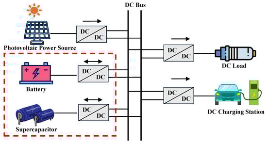
Figure 1. DC microgrid structure.

To enhance the transient performance of the system under disturbance conditions, this paper focuses on investigating control strategies for hybrid energy storage units. Figure 2 shows the structural diagram of the hybrid energy storage unit.

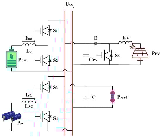
Figure 2. Hybrid energy storage system structure.

In Figure 2, $U_{dc}$ and C represent the bus-side voltage and capacitance, respectively; $P_{load}$ denotes the power required by the DC load; $P_{bat}$, $I_{bat}$, $L_b$, $S_1$, and $S_2$ represent the output power, inductor current, inductor, and switching transistor duty cycle on the battery side, respectively; $P_{sc}$, $I_{sc}$, $L_{sc}$, $S_3$, and $S_4$ represent the output power, inductor current, inductor, and switching transistor duty cycle on the supercapacitor side, respectively; $P_{pv}$, $I_{pv}$, $C_{pv}$, D, and $S_5$ represent the output power, inductor current, filter capacitance, and switching transistor duty cycle on the PV power supply side, respectively.

2.2. Low-Pass Filter Design

When the DC microgrid system is in a state of dynamic stability, the power relationships between the various units in the system are as follows:

$$P_{load}=P_{PV}+P_{HESS}$$

(1)

where $P_{PV}$ is the power provided by the photovoltaic array, $P_{HESS}$ is the power provided by the hybrid energy storage system, and $P_{load}$ is the power required by the load.

Therefore, the power of the HESS can be expressed as

$$P_{HESS}=P_{bat}+P_{sc}$$

(2)

where $P_{bat}$ is the power provided by the battery, $P_{sc}$ is the power provided by the supercapacitor.

As shown in Figure 2, The battery and supercapacitor are connected in parallel. Since line impedance is not considered in this article, power distribution can be equivalently treated as current distribution. The current distribution formula can be derived as follows:

$$I_{rHESS}=I_{bat}+I_{sc}$$

(3)

where $I_{bat}$ is the output current of the battery, $I_{sc}$ is the output current of the supercapacitor, and $I_{rHESS}$ is the total reference output current of the HESS.

Based on the fast response characteristic of supercapacitors, the reference current for the battery $I_{bat}$ can be obtained by subtracting the actual output current of the supercapacitor $I_{sc}$ from the total reference output current of the HESS $I_{rHESS}$, as follows:

$$I_{rbat}=I_{rHESS}-I_{sc}$$

(4)

Due to the relatively slow response speed of the battery, the uncompensated battery current $\Delta I_{bat}$ can be expressed as

$$\Delta I_{bat}=I_{rbat}-I_{bat}$$

(5)

By adding the uncompensated battery current to the reference current of the supercapacitor, the reference current for the supercapacitor $I_{rsc}$ can be derived as

$$I_{rsc}=I_{rHESS}(1-{\tau }_{LPF})+{\lambda }_{\Delta }{I}_{bat}$$

(6)

where ${\tau }_{LPF}$ is the low-pass filter value, $\lambda$ is the gain used to limit the battery current error, defined as $\lambda ={\displaystyle \frac{U_{bat}}{U_{sc}}}$, $U_{bat}$ is the terminal voltage of the battery, $U_{sc}$ is the terminal voltage of the supercapacitor.

Based on the above analysis, the control block diagram utilizing a low-pass filter to achieve frequency-based current distribution is shown in Figure 3.

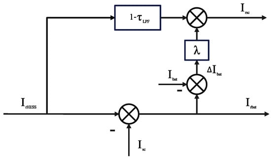
Figure 3. Block diagram of frequency reference current distribution control based on low-pass filter.

3. System Controller Design

3.1. Overview of PI Controller

Based on the aforementioned LPF current frequency division control, a traditional PI dual-closed-loop control strategy is adopted for the hybrid energy storage system. The control strategy diagram is shown in Figure 4.

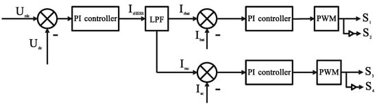
Figure 4. PI control structure diagram.

In the above figure, first, the bus voltage reference value $U_{rdc}$ is compared with the actual bus voltage value $U_{dc}$. The difference between the $U_{rdc}$ and the $U_{dc}$ is calculated. This difference is input into the voltage loop, where it undergoes PI control to generate a control signal. This control signal serves as the total current reference value $I_{rHESS}$ for the current loop. The $I_{rHESS}$ is input into an LPF low-pass filter for frequency division, yielding the low-frequency component battery current reference value $I_{rbat}$ and the high-frequency component supercapacitor current reference value $I_{rsc}$. In the battery current loop, the $I_{rbat}$ and $I_{bat}$ is calculated. This difference is input into a PI controller to determine the duty cycle of the battery switch, thereby regulating the battery output. The supercapacitor current loop operates similarly.

3.2. Overview of LADRC

Due to the inability to establish accurate mathematical models for hybrid energy storage systems, coupled with the random and fluctuating characteristics of photovoltaic-storage systems, PI control yields poor results. To enhance bus voltage control effectiveness, LADRC is introduced to improve the system’s interference resistance capability.

LADRC consists of a linear extended state observer (LESO) and a PD controller, offering the advantages of not relying on precise mathematical models of the system and possessing robust performance. The parameter configuration between the LESO and PD controller is linked to the bandwidth, which simplifies the tuning of control parameters. LESO estimates the total system disturbance through input and output signals and feeds the disturbance estimate back into the PD controller for compensation and elimination, thereby enhancing system stability.

The subject of this study can be treated as a second-order system.

$$\ddot{y}=-a_1\dot{y}-a_{2}y+\omega +bu$$

(7)

where u is the system input, which represents the total reference output current of HESS. y is the system output, which represents the actual bus voltage value. $\omega$ is the external disturbance, such as fluctuations in photovoltaic power supply and load disturbances. $a_1$ and $a_2$ are system parameters, b is the system gain, and $a_1$ and $a_2$ are unknown. In the design of detectors, the precise value of b is difficult to obtain, so it is typically replaced with its estimated value $b_0$; therefore $b_0\approx b$.

Let $f(y,\dot{y},\omega )$ denote the total disturbance to the system, which can be expressed as $f(y,\dot{y},\omega )=-a_1\dot{y}-a_{2}y+\omega +\left(b-b_0\right)u$. Therefore, after separating the total disturbance from the system, the system is derived as

$$\begin{array}{cc}\hfill \ddot{y}& =b_{0}u+f(y,\dot{y},\omega )\hfill \end{array}$$

(8)

According to ESO design principles, first define the state variable $x_1=y$, whose first derivative is $x_2=\dot{y}$, and expand the disturbance term f into a new state variable $x_3$ for the system. Then, the system’s state equation can be obtained as

$$\left\{\begin{array}{c}{\dot{x}}_1=x_2\hfill \\ {\dot{x}}_2=x_3+b_{0}u\hfill \\ {\dot{x}}_3=\dot{f}\hfill \\ x_1=y=U_{dc}\hfill \end{array}\right.$$

(9)

The LESO designed based on Equation (9) is expressed as

$$\left\{\begin{array}{c}{e}_z=z_1-y\hfill \\ {\dot{z}}_1=z_2-{\theta }_1{e}_z\hfill \\ {\dot{z}}_2=z_3-{\theta }_2{e}_z+b_{0}u\hfill \\ {\dot{z}}_3=-{\theta }_3{e}_z\hfill \end{array}\right.$$

(10)

where $e_z$ is the DC bus voltage tracking error of LESO, $z_1$, $z_2$, and $z_3$ are the observed values of the state variables $x_1$, $x_2$, and $x_3$, respectively; moreover, ${\theta }_1$, ${\theta }_2$, and ${\theta }_3$ are the gains of the first-level observer, all of which are positive.

To simplify parameter design, the gain configuration of LESO is as follows:

$$\left\{\begin{array}{c}{\theta }_1=3{\omega }_0\hfill \\ {\theta }_2=3{\omega }_0^2\hfill \\ {\theta }_3={\omega }_0^3\hfill \end{array}\right.$$

(11)

where ${\omega }_0$ is the observer bandwidth.

By observing the state variables of the LESO system in real time, a disturbance compensation stage is designed based on the concept of self-disturbance rejection to eliminate disturbances. This transforms the system with uncertain disturbances into an equivalent integrated series system. The disturbance compensation stage is designed as follows:

$$u={\displaystyle \frac{u_0-z_3}{b_0}}$$

(12)

Substituting above equation into Equation (8) and neglecting estimation errors yields

$$\ddot{y}=u_0-z_3+f$$

(13)

Inputting the observed state variable into the PD controller yields the control law:

$$u_0=k_p(v-z_1)-k_d{z}_2$$

(14)

where v represents the system input reference value; $k_p$ and $k_d$ denote the controller gains to be designed.

Substituting above equation into Equation (13) and rearranging yields the input–output relationship of the system:

$$\ddot{y}=k_p(v-z_1)-k_d{z}_2$$

(15)

In summary, the LADRC structure diagram is shown in Figure 5.

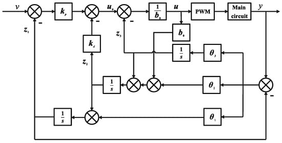
Figure 5. LADRC control structure diagram.

LADRC employs a linear observer to estimate the total disturbance in real time, designing a controller to compensate and eliminate it. However, for traditional ESO, increasing bandwidth can enhance estimation performance and reduce the overall impact of disturbances. Due to limitations imposed by measurement noise and system stiffness, the bandwidth cannot be set excessively high. Moreover, traditional ESO can only guarantee asymptotic convergence of estimation errors to zero, which results in relatively slow convergence speed and limited accuracy. And its PD control approach, while reducing parameter tuning complexity, suffers from poor compensation accuracy and response speed.

3.3. Design of CESO

In this paper, the voltage loop and current loop adopt the same control strategy. Therefore, subsequent designs will use the voltage loop as an example. CESO can rapidly and accurately reconstruct signals while avoiding excessive amplification of measurement noise. Therefore, to address this issue, this section designs CESO to enhance the performance of a traditional ESO.

Based on the core concept of LADRC, which treats uncertainties in the system model as total disturbance and performs unified real-time estimation and compensation alongside internal and external disturbances through an extended state observer; this paper sets the nominal control gain $b_0$ to 1.

Substituting $b_0=1$ into Equation (8), the system is derived as

$$\begin{array}{cc}\hfill \ddot{y}& =b_{0}u+f(y,\dot{y},\omega )\hfill \\ \hfill & =u+f(y,\dot{y},\omega )\hfill \end{array}$$

(16)

According to LESO design principles, first define the state variable $x_1=y$, whose first derivative is $x_2=\dot{y}$, and expand the disturbance term f into a new state variable $x_3$ for the system. Then, the system’s state equation can be obtained as

$$\left\{\begin{array}{c}{\dot{x}}_1=x_2\hfill \\ {\dot{x}}_2=x_3+u\hfill \\ {\dot{x}}_3=\dot{f}\hfill \\ x_1=y=U_{dc}\hfill \end{array}\right.$$

(17)

The first-level observer ESO1 designed based on Equation (17) is expressed as

$$\left\{\begin{array}{c}{e}_g=g_1-y\hfill \\ {\dot{g}}_1=g_2-{\xi }_1{e}_g\hfill \\ {\dot{g}}_2=g_3-{\xi }_2{e}_g+u\hfill \\ {\dot{g}}_3=-{\xi }_3{e}_g\hfill \end{array}\right.$$

(18)

where $e_g$ is the DC bus voltage tracking error of ESO1, $g_1$, $g_2$, and $g_3$ are the observed values of the state variables $x_1$, $x_2$, and $x_3$, respectively; moreover, ${\xi }_1$, ${\xi }_2$, and ${\xi }_3$ are the gains of the first-level observer, all of which are positive.

To further enhance the observer performance, the observed value of the total disturbance obtained from ESO1 is introduced into the second-level observer ESO2 as a known component for feedforward compensation. Thus, Equation (18) can be reconstructed as

$$\left\{\begin{array}{c}{e}_v=v_1-y\hfill \\ {\dot{v}}_1=v_2-{\eta }_1{e}_v\hfill \\ {\dot{v}}_2=v_3-{\eta }_2{e}_v+u+g_3\hfill \\ {\dot{v}}_3=-{\eta }_3{e}_v\hfill \end{array}\right.$$

(19)

where $e_v$ is the DC bus voltage tracking error of ESO2, $v_1,v_2$, and $v_3$ are the observed values of the state variables of ESO2, respectively; and ${\eta }_1$, ${\eta }_2$, and ${\eta }_3$ are gains of ESO2, all of which are positive.

By constructing front and rear cascaded observers, the state estimation results from the front-level observer are utilized to dynamically adjust the rear-level observer, enabling rapid collaborative tracking of disturbance components. To simplify parameter design, the gains of both observers are configured as follows:

$$\left\{\begin{array}{c}{\xi }_1={\eta }_1=3{\omega }_0\hfill \\ {\xi }_2={\eta }_2=3{\omega }_0^2\hfill \\ {\xi }_3={\eta }_3={\omega }_0^3\hfill \end{array}\right.$$

(20)

where ${\omega }_0$ is the observer bandwidth.

3.4. Design of FxADRC

The purpose of this paper is to achieve precise tracking of the desired bus voltage under uncertain disturbances via the fixed-time methods. The input of the controller is the desired bus voltage, and the output is the total reference output current of the HESS.

By synthesizing the observed values $g_3$ and $v_3$ in real time, information about the total disturbance f was reconstructed. The following FxADRC is introduced for the system:

$$u=u_1+u_2-(g_3+v_3)$$

(21)

The bus voltage tracking error can be defined as

$$e=\sigma -v_1$$

(22)

where $\sigma$ denotes the desired bus voltage.

Take the derivative of Equation (22), which yields

$$\dot{e}=\dot{\sigma }-{\dot{v}}_1$$

(23)

The $u_1$ is designed to ensure fixed-time stability within a small error range of the system as follows:

$$u_1=-k_{1}e-k_2\dot{e}$$

(24)

where $k_1>0$, $k_2>0$.

The $u_2$ is designed to accelerate system response as follows:

$$u_2=-k_{51}{sgn\left(s\right)\left|s\right|}^{\alpha }-k_{52}sgn\left(s\right){\left|s\right|}^{\beta }$$

(25)

where $k_{51},k_{52}$ are gain coefficients, $k_{51}>0$, $k_{52}>0$, $\alpha$, and $\beta$ are constants satisfying, $0<\alpha <1$ and $\beta >1$.

The slipform surface s can be defined as

$$s=k_{3}e-\psi$$

(26)

where $k_3$ is gain coefficient, $k_3>0$, $\psi$ is dynamic integral term, which can be expressed as

$$\psi ={\int }_0^t\left[k_{41}{sgn\left(s\right)\left|s\right|}^{\alpha }+k_{42}sgn\left(s\right){\left|s\right|}^{\beta }\right]dt$$

(27)

where $k_{41},k_{42}$ are gain coefficients, $k_{41}>0$, $k_{42}>0$.

Substituting Equations (24) and (25) into Equation (21) yields

$$u=-k_{1}e-k_2\dot{e}-k_{51}{sgn\left(s\right)\left|s\right|}^{\alpha }-k_{52}sgn\left(s\right){\left|s\right|}^{\beta }-g_3-v_3$$

(28)

In summary, the control structure block diagram of the hybrid energy storage system in the photovoltaic-storage DC microgrid is shown in Figure 6.

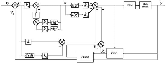
Figure 6. Block diagram of voltage ring FxADRC.

4. Stability Proof

In order to validate the convergence characteristic of proposed controller, the Lyapunov method is utilized in this section. The stability analysis of the voltage loop is presented as an example, and the stability analysis of the current loop is similar with the voltage loop.

4.1. Stability Proof of CLESO

The following standard lemma is first introduced to support the subsequent analysis.

Lemma 1.

Considering the system $\dot{x}=f(x,t)$. If there exists a continuous radially unbounded function $V\left(x\right):{\mathbb{R}}^n\to {\mathbb{R}}_{\ge 0}$ such that, $V\left(x\right)>0forallx\ne 0,andV\left(0\right)=0$, $\dot{V}\left(x\right)\le -\kappa V\left(x\right)+\theta$, where $\kappa >0and\theta >0$. Then, the system is uniformly ultimately bounded.

The observation errors of ESO1 are defined as

$$\left\{\begin{array}{c}{e}_{g1}=g_1-x_1\hfill \\ e_{g2}=g_2-x_2\hfill \\ e_{g3}=g_3-x_3\hfill \end{array}\right.$$

(29)

Taking the derivative of the above equation and substituting them into Equation (18) yields the error dynamics:

$$\left\{\begin{array}{c}{\dot{e}}_{g1}=e_{g2}-{\xi }_1{e}_{g1}\hfill \\ {\dot{e}}_{g2}=e_{g3}-{\xi }_2{e}_{g1}\hfill \\ {\dot{e}}_{g3}=-{\xi }_3{e}_{g1}-\dot{f}\hfill \end{array}\right.$$

(30)

Then, the above error dynamics can be transformed to a matrix form as:

$${\dot{e}}_g=A_g{e}_g+B_g\dot{f}$$

(31)

where $e_g={\left[e_{g1},e_{g2},e_{g3}\right]}^T.$ And where

$$A_g=\left[\begin{array}{ccc}-{\xi }_1& 1& 0\\ -{\xi }_2& 0& 1\\ -{\xi }_3& 0& 0\end{array}\right],B_g=\left[\begin{array}{c}0\\ 0\\ -1\end{array}\right]$$

(32)

The observer gains are chosen as ${\xi }_1=3{\omega }_0$, ${\xi }_2=3{\omega }_0^2$, ${\xi }_3={\omega }_0^3$, and $A_g$ is the Hurwitz matrix. Therefore, for any symmetric positive definite matrix $Q_g$, there exists a symmetric positive definite matrix $P_g$ satisfying the Lyapunov function:

$$A_g^T{P}_g+P_g{A}_g=-Q_g$$

(33)

A Lyapunov Function is defined as

$$V_g=e_g^T{P}_g{e}_g$$

(34)

and its time derivative satisfies

$$\begin{array}{cc}\hfill {\dot{V}}_g& =e_g^T\left(A_g^T{P}_g+P_g{A}_g\right)e_g+2e_g^T{P}_g{B}_g\dot{f}\hfill \end{array}$$

(35)

Substituting above equation into Equation (33) gives

$${\dot{V}}_g=-e_g^T{Q}_g{e}_g+2e_g^T{P}_g{B}_g\dot{f}$$

(36)

Assume that the derivative of the total disturbance is bounded ($\exists L>0$,$|\dot{f}|\le L$); using the Cauchy–Schwarz inequality,

$${\dot{V}}_g\le -{\lambda }_{min}\left(Q_g\right){\parallel e_g\parallel }^2+2\parallel P_g{B}_g\parallel L\parallel e_g\parallel$$

(37)

Let $∥e_g∥\ge {\displaystyle \frac{4∥P_g{B}_g∥L}{{\lambda }_{min}\left(Q_g\right)}}$), then

$${\dot{V}}_g\le -{\displaystyle \frac{1}{2}}{\lambda }_{min}\left(Q_g\right){\parallel e_g\parallel }^2$$

(38)

Since $V_g$ is quadratic form, there exist $c_1>0,c_2>0$, such that $c_1{∥e_g∥}^2\le V_g\le c_2{∥e_g∥}^2$. Therefore,

$${\dot{V}}_g\le -{\displaystyle \frac{{\lambda }_{min}\left(Q_g\right)}{2c_2}}{V}_g$$

(39)

which implies that when $\parallel e_g\parallel$ is sufficiently large, ${\dot{V}}_g$ is negative definite. According to Lemma 1, the observation errors of ESO1 are uniformly ultimately bounded.

Following the rigorous framework established by ESO1, this paper presents a stability proof for ESO2.

The observation errors of ESO2 are defined as

$$\left\{\begin{array}{c}{e}_{v1}=v_1-x_1\hfill \\ e_{v2}=v_2-x_2\hfill \\ e_{v3}=v_3-x_3\hfill \end{array}\right.$$

(40)

Taking the derivative of the above equation and substituting them into Equation (19) yields the following error dynamics:

$$\left\{\begin{array}{c}{\dot{e}}_{v1}=e_{v2}-{\eta }_1{e}_{v1}\hfill \\ {\dot{e}}_{v2}=e_{v3}-{\eta }_2{e}_{v1}+e_{g3}\hfill \\ {\dot{e}}_{v3}=-{\eta }_3{e}_{v1}-\dot{f}\hfill \end{array}\right.$$

(41)

Then, the above error dynamics can be transformed to a matrix form as

$${\dot{e}}_v=A_v{e}_v+B_v\dot{f}+D{e}_{g3}$$

(42)

where $e_v={\left[e_{v1},e_{v2},e_{v3}\right]}^T$ and where

$$A_v=\left[\begin{array}{ccc}-{\eta }_1& 1& 0\\ -{\eta }_2& 0& 1\\ -{\eta }_3& 0& 0\end{array}\right],B_v=\left[\begin{array}{c}0\\ 0\\ -1\end{array}\right],D=\left[\begin{array}{c}0\\ 1\\ 0\end{array}\right]$$

(43)

The observer gains are chosen as ${\eta }_1=3{\omega }_0$, ${\eta }_2=3{\omega }_0^2$, ${\eta }_3={\omega }_0^3$, and $A_v$ is the Hurwitz matrix. Therefore, for any symmetric positive definite matrix $Q_v$, there exists a symmetric positive definite matrix $P_v$ satisfying the Lyapunov Function:

$$A_v^T{P}_v+P_v{A}_v=-Q_v$$

(44)

A Lyapunov Function is defined as

$$V_v=e_v^T{P}_v{e}_v$$

(45)

and its time derivative satisfies

$${\dot{V}}_v=e_v^T\left(A_v^T{P}_v+P_v{A}_v\right)e_v+{\left(B_v\dot{f}+D{e}_{g3}\right)}^T{P}_v{e}_v+e_v^T{P}_v\left(B_v\dot{f}+D{e}_{g3}\right)$$

(46)

Substituting the above equation into Equation (44) gives

$${\dot{V}}_v=-e_v^T{Q}_v{e}_v+2e_v^T{P}_v\left(B_v\dot{f}+D{e}_{g3}\right)$$

(47)

According to the Cauchy–Schwarz inequality and the properties of matrix norms, it can be concluded that

$$2e_v^T{P}_v\left(B_v\dot{f}+D{e}_{g3}\right)\le 2∥P_v∥∥e_v∥∥B_v\dot{f}+D{e}_{g3}∥$$

(48)

Assume that the derivative of the total disturbance is bounded ($\exists Lv>0$,$|\dot{f}|\le L_v$). At the same time, it follows from the stability proof of ESO1 that its observational error $e_{g3}$ is ultimately bounded. Therefore, the norm of the disturbance term can be estimated as

$$∥B_v\dot{f}+D{e}_{g3}∥=∥{[0,e_{g3},-\dot{f}]}^T∥=\sqrt{{\left(e_{g3}\right)}^2+{\left(\dot{f}\right)}^2}\le \sqrt{L^2+L_v^2}=L_{\varphi }$$

(49)

Substituting the above equation into Equation (47) gives

$${\dot{V}}_v\le -{\lambda }_{min}\left(Q_v\right){∥e_v∥}^2+2∥P_v∥L_{\varphi }∥e_v∥$$

(50)

Let $∥e_v∥>{\displaystyle \frac{2∥P_v∥L_{\varphi }}{{\lambda }_{min}\left(Q_v\right)}}$, from Equation (50), it can be seen that:

$${\dot{V}}_v<0$$

(51)

According to Lemma 1, the observation errors of ESO2 are uniformly ultimately bounded.

4.2. Stability Proof of FxADRC

Considering the system, Equation (16) under the controller Equation (24), the closed-loop system is fixed-time stable. Specifically, the bus voltage tracking error e and its derivative $\dot{e}$ will converge to a small region near the origin within a fixed time, and the upper bound on convergence time $T_{max}$ is independent of the system’s initial state.

The Lyapunov function is considered as follows:

$$V={\displaystyle \frac{1}{2}}{s}^2$$

(52)

which is obviously positive definite and radially unbounded. Then, the derivative of V is given by

$$\dot{V}=s\dot{s}$$

(53)

Substituting Equation (27) into Equation (26) yields the derivative.

$$\begin{array}{cc}\hfill \dot{V}& =s·\left[k_3\dot{e}-k_{41}{sgn\left(s\right)\left|s\right|}^{\alpha }-k_{42}sgn\left(s\right){\left|s\right|}^{\beta }\right]\hfill \\ \hfill & =s·\left(k_3\dot{e}\right)-k_{41}s·{sgn\left(s\right)\left|s\right|}^{\alpha }-k_{42}s·sgn\left(s\right){\left|s\right|}^{\beta }\hfill \end{array}$$

(54)

Using the Equation $s·sgn\left(s\right)=\left|s\right|$, the above equation can be simplified to

$$\dot{V}=s·\left(k_3\dot{e}\right)-k_{41}{\left|s\right|}^{\alpha +1}-k_{42}{\left|s\right|}^{\beta +1}$$

(55)

Under the action of the designed control law, the error dynamics of the closed-loop system can be characterized as

$$k_3\dot{e}=-Ks+\tilde{d}$$

(56)

where K is the overall feedback gain. $K>0$, $\tilde{d}$ denotes the bounded residual disturbance estimation error after CESO compensation, $|\tilde{d}|\le D$.

Substituting the above equation into Equation (55) yields

$$\begin{array}{cc}\hfill \dot{V}& =s·(-Ks+\tilde{d})-k_{41}{\left|s\right|}^{\alpha +1}-k_{42}{\left|s\right|}^{\beta +1}\hfill \\ \hfill & =-K{s}^2+s\tilde{d}-k_{41}{\left|s\right|}^{\alpha +1}-k_{42}{\left|s\right|}^{\beta +1}\hfill \end{array}$$

(57)

Using $s^2={\left|s\right|}^2$ and $s\tilde{d}\le \left|s\right|D$, we can scale the above expression to obtain

$$\dot{V}\le -{K\left|s\right|}^2+D\left|s\right|-k_{41}{\left|s\right|}^{\alpha +1}-k_{42}{\left|s\right|}^{\beta +1}$$

(58)

By selecting a sufficiently large controller gain, the system state can be ensured to be attracted to the region $\left|\mathit{s}\right|\le \Delta$ within a fixed time. Where $\Delta$ is a constant related to the disturbance upper bound D.

To prove fixed-time convergence, the above equation is transformed into an expression in terms of the Lyapunov function V. Given that $V={\displaystyle \frac{1}{2}}{s}^2$, it follows that $\left|s\right|=\sqrt{2}{V}^{1/2}$. By defining ${\eta }_{11}={\displaystyle \frac{\alpha +1}{2}}$ and ${\eta }_{12}={\displaystyle \frac{\beta +1}{2}}$, and substituting the above equations into Equation (59), we obtain

$$\dot{V}\le -2KV+\sqrt{2}D{V}^{1/2}-k_{41}{2}^{{\eta }_{11}}{V}^{{\eta }_{11}}-k_{42}{2}^{{\eta }_{12}}{V}^{{\eta }_{12}}$$

(59)

Given the constraints $0<\alpha <1$ and $\beta >1$, the parameters are bounded as $1/2<{\eta }_{11}<1$ and ${\eta }_{12}>1$. Using standard inequality scaling techniques, it can be demonstrated that there exist positive constants ${\gamma }_1$ and ${\gamma }_2$, such that

$$\dot{V}\le -{\gamma }_1{V}^{{\eta }_{11}}-{\gamma }_2{V}^{{\eta }_{12}}$$

(60)

According to the fixed-time stability theorem [27], the system state will converge within a fixed time T. The settling time T is upper-bounded by

$$T\le T_{max}={\displaystyle \frac{1}{{\gamma }_1(1-{\eta }_{11})}}+{\displaystyle \frac{1}{{\gamma }_2({\eta }_{12}-1)}}$$

(61)

Crucially, this upper bound $T_{max}$ is independent of the initial state of the system, which completes the proof of fixed-time convergence.

5. Simulation Verification of Disturbance Rejection Under Different Control Strategies

This section constructs a hybrid energy storage simulation model for a photovoltaic-integrated mainstream microgrid on the Matlab/Simulink platform to verify the feasibility of the proposed control method. To better evaluate the response speed and disturbance rejection capability of the designed controller, comparative analyses are conducted with PI control and LADRC control under unchanged electrical model parameters. The initial system conditions are set as follows: ambient temperature of 25 °C, irradiance of 1000 W/m², with the photovoltaic unit employing MPPT control. The constant of the low-pass filter ${\tau }_{\mathrm{LPF}}$ is 0.005. The selection of the low-pass filter time constant ${\tau }_{\mathrm{LPF}}$ set to 0.005 plays a critical role in the frequency-based current distribution between the battery and supercapacitor. This value was chosen based on typical configurations from the literature [7,8,9,10,11] to balance the trade-off between dynamic response and noise immunity. Smaller ${\tau }_{\mathrm{LPF}}$ values increase filter bandwidth, enabling faster tracking of high-frequency disturbances such as rapid load changes or PV fluctuations, but may amplify measurement noise and cause overshoot. Conversely, larger ${\tau }_{\mathrm{LPF}}$ values smooth current distribution but introduce delays, potentially degrading transient response performance under changing operating conditions. In this study, setting ${\tau }_{\mathrm{LPF}}$ = 0.005 effectively decouples the slow dynamics of the battery from the fast response of the supercapacitor, thereby enhancing bus voltage stability. The system model parameters are listed in Table 1. The simulation parameter settings for each controller are listed in Table 2.

Table 1. System model parameters.

Model Parameters	Unit	Value
DC Bus Reference Voltage	V	700
DC-Link Capacitor	F	0.001
Initial Terminal Voltage of the Supercapacitor	V	300
Initial Terminal Voltage of the Battery	V	200
Supercapacitor-Side Inductance	H	0.01
Battery-Side Inductance	H	0.01

The parameter values are based on typical configurations from [7,11].

Table 2. Parameters of each controller.

Controller	Parameters of Voltage Loop	Parameters of Current Loop
PI	$K_{\mathrm{i}1}=15$	$K_{\mathrm{i}2}=0.5$
	$K_{\mathrm{p}1}=0.5$	$K_{\mathrm{p}2}=105$
LADRC	${\omega }_0=314,b_0=240$	${\omega }_0=3140,b_0=240$
	$k_{\mathrm{p}}=50,k_{\mathrm{d}}=2500$	$k_{\mathrm{p}}=50,k_{\mathrm{d}}=2500$
FxADRC-CESO	$k_1=8,k_2=323,k_3=10$	$k_1=8,k_2=323,k_3=10$
	$k_{41}=2,k_{42}=0.5,$	$k_{41}=2,k_{42}=0.5,$
	$k_{51}=1000,k_{52}=5800,$	$k_{51}=1000,k_{52}=5800,$
	$\alpha =0.45,\beta =1.4,$	$\alpha =0.45,\beta =1.4,$
	${\omega }_0=3140$	${\omega }_0=31400$

The PI control strategy employs the Ziegler–Nichols method [22]. The optimal tuning parameters for the PI controller were obtained through empirical formulas. LADRC sets the bandwidths of the controller and observer individually and tunes them according to the bandwidth method [23], obtaining the optimal bandwidth parameters. Regarding the control strategy proposed in this paper, during parameter tuning, the principle of observation before control should be followed. Since the observer is a CESO, its parameter design has been simplified, requiring only adjustment of ${\omega }_0$. The gradually increasing ${\omega }_0$ accelerates the observer’s convergence speed and enhances disturbance estimation capability. The tuning should ultimately achieve rapid convergence of the observation error without significant overshoot. Considering the linear portion of Equation (24), tune $k_1$ and $k_2$ based on PD control to achieve steady-state tracking performance. Next, fix exponents $\alpha$ and $\beta$, then incrementally increase $k_{51}$ and $k_{52}$ to ensure the system converges to steady-state within a fixed upper time limit independent of initial conditions. Finally, fine-tune $k_3$, $k_{41}$, and $k_{42}$ to further enhance performance.

5.1. Photovoltaic Power Disturbance Simulation Comparison

The load maintains a constant power operation at 2.5 kW, while the irradiance varies as shown in Figure 7.

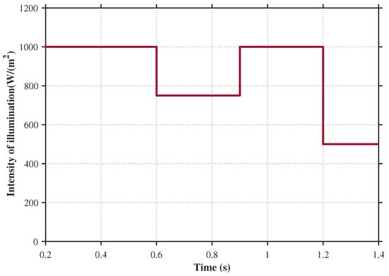
Figure 7. Variation in light intensity.

The variation in the output power of the photovoltaic source is shown in Figure 8.

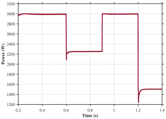
Figure 8. Photovoltaic power supply output power.

Analysis of the above two figures indicates that at t = 0.6 s when the irradiance drops from 1000 W/m² to 750 W/m², and the photovoltaic output power becomes lower than the load demand power, leading to a decrease in bus voltage. At this point, the hybrid energy storage unit compensates for the power deficit. At t = 0.9 s, when the irradiance abruptly changes from 750 W/m² to 1000 W/m², the photovoltaic output power exceeds the load demand power, causing a momentary rise in bus voltage. The hybrid energy storage unit absorbs the surplus power to maintain bus voltage stability. At t = 1.2 s, when the irradiance suddenly drops from 1000 W/m² to 500 W/m², the bus voltage instantaneously decreases but is restored to equilibrium through compensation by the energy storage unit. For photovoltaic power disturbances, under unchanged controller parameters, three control strategies are compared and analyzed as follows.

Comparison of DC Bus Voltage Simulation

A comparison of DC bus voltage waveforms under different control strategies during photovoltaic power disturbances is shown in Figure 9.

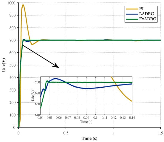
Figure 9. DC bus voltage starting waveform during photovoltaic power disturbance.

The simulation result in Figure 9 reveals that the maximum voltage peaks under the PI, LADRC and FxADRC control strategies were $983.96\mathrm{V}$, $706.58\mathrm{V}$, and $701.67\mathrm{V}$, respectively, with voltage overshoot values of $283.96\mathrm{V}$, $6.58\mathrm{V}$, and $1.67\mathrm{V}$, respectively. Compared to PI control, the overshoot of the LADRC control strategy is reduced by $97.68\%$, while the FxADRC control strategy achieves a reduction of $99.41\%$. And the settling times were $0.34\mathrm{s}$, $0.21\mathrm{s}$, and $0.05\mathrm{s}$, respectively. Compared to PI control, the adjustment time of the LADRC control strategy is reduced by $38.24\%$, while that of the FxADRC control strategy is reduced by $85.29\%$. As shown in Table 3. Comparing the above simulation results, it can be seen that the FxADRC strategy proposed in this paper exhibits smaller overshoot and faster transient response speed during photovoltaic power disturbances.

Table 3. Performance comparison of different control strategies under photovoltaic disturbances.

Controller	Stability Time (s)	Stability Time Reduction (%)	Overshoot (V)	Overshoot Reduction (%)
PI	0.34	—	283.96	—
LADRC	0.21	38.24	6.58	97.68
FxADRC	0.05	85.29	1.67	99.41

Figure 10 illustrates the comparative suppression effects of different control strategies on DC bus voltage disturbance waveforms during photovoltaic power disturbances. The simulation results under the PI control, LADRC, and FxADRC strategies are shown in (a), (b), and (c), respectively.

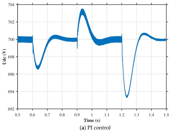
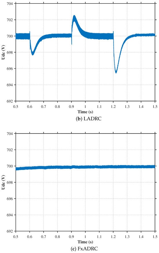
Figure 10. Comparison of DC bus voltage waveform during photovoltaic power disturbance.

Taking the scenario at $t=0.9$ s as an example, when the irradiance abruptly increases from 750 W/m² to 1000 W/m², the photovoltaic output power exceeds the load demand power, causing a bus voltage surge. Under PI control, the bus voltage surges by $3.43$ V and stabilizes after 112 ms. Under LADRC control, the surge is $2.37$ V with stabilization achieved in 83 ms. Whereas under FxLADRC control, the voltage surge is significantly smaller at $0.05$ V, with stabilization in just 19 ms. These results demonstrate that the proposed FxADRC strategy achieves smaller bus voltage fluctuations and faster transient recovery during photovoltaic power disturbances.

5.2. Load Power Disturbance Simulation Comparison

Under the condition that the photovoltaic output power remains constant at 3 kW, the variations in load output power are illustrated in Figure 11.

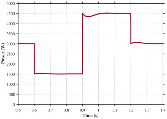
Figure 11. Load output power fluctuation.

Comparison of DC Bus Voltage Simulation

A comparison of DC bus voltage waveforms under different control strategies during load power disturbances is shown in Figure 12.

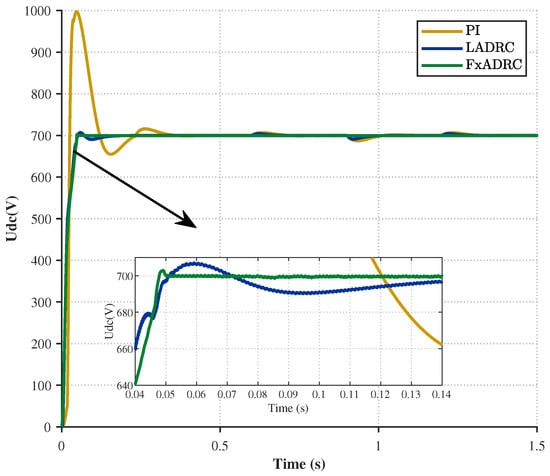
Figure 12. DC bus voltage starting waveform during load power perturbation.

The analysis of Figure 12 clearly shows that there is a difference in performance between the three strategies. The PI controller yielded the poorest results. It had a high voltage peak of $997.97\mathrm{V}$. It also had an overshoot of $297.97\mathrm{V}$. And it had a slow settling time of $0.38\mathrm{s}$. The LADRC strategy provided a significant improvement, reducing the overshoot to $8.45\mathrm{V}$ with a peak voltage of $708.45\mathrm{V}$ and reducing the settling time to $0.26\mathrm{s}$. The FxADRC method achieved superior performance by limiting the overshoot to just $2.39\mathrm{V}$ with a peak voltage of and $702.39\mathrm{V}$ and achieving a settling time of $0.05\mathrm{s}$. Compared to the PI control strategy, the overshoot under the LADRC control strategy is reduced by $97.17\%$, and the settling time is shortened by $31.58\%$. While the overshoot under the FxADRC control strategy is reduced by $99.20\%$, and the settling time is shortened by $86.84\%$. As shown in Table 4. A comparison of these simulation results shows that the proposed FxADRC strategy results in smaller overshoot and a faster transient response during load power disturbances.

Table 4. Performance comparison of different control strategies under load disturbances.

Controller	Stability Time (s)	Stability Time Reduction (%)	Overshoot (V)	Overshoot Reduction (%)
PI	0.38	—	297.97	—
LADRC	0.26	31.58	8.45	97.17
FxADRC	0.05	86.84	2.39	99.20

Figure 13 illustrates the comparison of suppression effects on DC bus voltage disturbance waveforms among different control strategies during load power disturbances. The simulation results under the PI control, LADRC, and FxADRC strategies are shown in (a), (b), and (c), respectively.

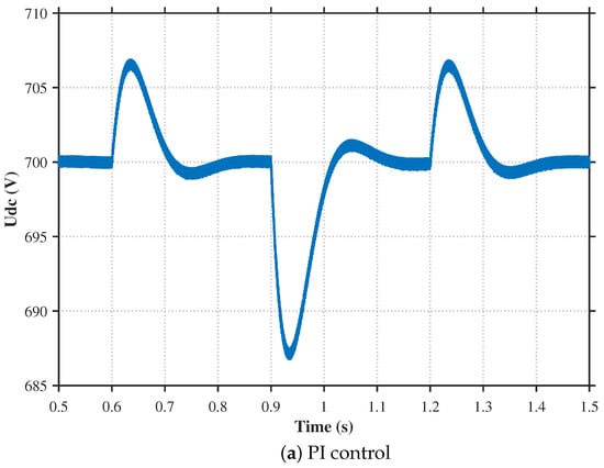
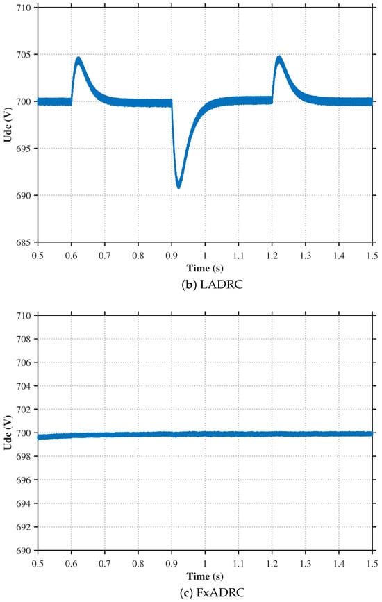
Figure 13. Comparison of DC bus voltage waveform during load power disturbance.

Considering the scenario at $t=0.9$ s, the system load power suddenly increases from $1.5$ kW to $4.5$ kW. As the load demand power exceeds the photovoltaic output power, the DC bus voltage drops, and the energy storage unit compensates for the power deficit to stabilize the bus voltage. Analysis of Figure 13 reveals that under PI control, the bus voltage drops to $13.21$ V and stabilizes after 132 ms; under LADRC control, the voltage drops to $9.19$ V and stabilizes in 111 ms; whereas under FxADRC control, the voltage drop is only $0.35$ V with stabilization achieved in just 34 ms. These results demonstrate that the proposed FxADRC strategy achieves smaller bus voltage fluctuations and faster transient recovery during power disturbances.

5.3. Verification and Analysis of Fixed-Time Convergence

To verify that the proposed FxADRC control strategy converges within a fixed time, simulations were conducted as follows: while keeping all other controller parameters and disturbances constant, only the initial conditions were varied, i.e., 650 V, 700 V, and 750 V. The simulation results are shown in Figure 14.

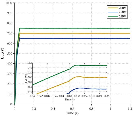
Figure 14. Comparison of DC bus voltage under different initial conditions.

Analysis of Figure 14 reveals that under initial conditions of 650 V, 700 V, and 750 V, respectively, all systems converge within a fixed time of 0.05 s. This further validates the proposed control strategy’s capability to converge within a fixed timeframe, demonstrating its superiority.

5.4. Robustness Analysis Based on Theoretical Framework

To validate the stability of the FxADRC control strategy under complex environmental conditions such as ambient temperature fluctuations or irregular illumination, the following analysis was conducted.

Based on the Lyapunov stability proof, both the CESO and FxADRC ensure that system errors converge to a small neighborhood near the origin within a fixed time, with this convergence property independent of initial conditions. This convergence is guaranteed under the assumption that the total disturbance acting on the system is bounded, as formalized in Lemma 1. Specifically, this proof demonstrates that the derivative of the total disturbance satisfies $|\dot{f}|\le L$. The cascaded structure of the CESO, comprising primary and secondary observers for residual compensation, enables real-time estimation and suppression of these disturbances, thereby ensuring the closed-loop system exhibits uniform ultimate boundedness. Complex environmental factors such as temperature variations or irregular solar radiation can be abstracted as bounded perturbations within this theoretical framework. For instance, temperature fluctuations may induce slow-varying perturbations in photovoltaic efficiency or cell dynamics, while irregular radiation introduces high-frequency random components. However, since these effects are physically constrained and, thus, bounded, the controller derived from the Lyapunov function derivative inequality (60) maintains fixed-time convergence properties. This feature ensures that the design gain dominates the worst-case disturbance boundary. Consequently, the FxADRC scheme maintains its robustness even in complex environments.

6. Conclusions

This paper addresses the issue of bus voltage fluctuations in hybrid energy storage systems under system uncertainties and external disturbances by proposing the FxADRC method based on the CESO. First, a dynamic model of the DC bus voltage incorporating external disturbances is constructed. Subsequently, the CESO is designed to estimate and compensate for system disturbances, thereby enhancing robustness. FxADRC is then implemented for both the current and voltage loops, enabling error convergence within a fixed time period independent of the system’s initial state. Furthermore, the stability of the proposed control method is analyzed using the Lyapunov approach, proving that the control strategy achieves fixed-time convergence. Finally, simulations compare the proposed control strategy with PI control and conventional ADRC control, verifying its effectiveness and superiority.

Although simulation results demonstrate the effectiveness of the proposed FxADRC strategy in suppressing bus voltage fluctuations under various disturbances, certain limitations exist. For instance, practical application still requires validation through field testing in real HESS systems. To address these limitations, we will enhance simulation experiments of the control strategy under complex conditions. Subsequently, we will design and construct a hardware platform integrating photovoltaic ports, hybrid energy storage ports, DC load ports, and grid ports to validate the effectiveness of the proposed experimental strategy.

References

- Jiang, F.; Yin, Z.; Hu, W.; Cui, C.; He, R.; Huang, S. A Review of Control Strategies for AC Microgrids with Distribution Network-Microgrid Coordination. J. Electr. Eng. 2025, 20, 225–242. [Google Scholar]
- Su, H.; Li, K.; Yang, F.; Zhu, Y. Multi-Criteria Integrated Decision-Making for Power Grid Planning with High Penetration of Renewable Energy Integration. Electron. Des. Eng. 2025, 33, 174–178. [Google Scholar]
- Zhang, Z.; Luo, C.; Zhang, G.; Shu, Y.; Shao, S. New energy policy and green technology innovation of new energy enterprises: Evidence from China. Energy Econ. 2024, 136, 107743. [Google Scholar] [CrossRef]
- Xie, X.; Ma, N.; Liu, W.; Zhao, W.; Xu, P.; Li, H. A Review and Prospects of Energy Storage Application Functions in New-Type Power Systems. Proc. CSEE 2023, 43, 158–169. [Google Scholar]
- Zhu, X.; Jiang, Q.; Liu, M.; Luo, H.; Long, W.; Huang, L. Two-Stage Optimal Scheduling of Integrated Energy Systems Considering Source-Load Uncertainty. Electr. Power Autom. Equip. 2023, 43, 9–16+32. [Google Scholar]
- Hu, G.; Li, Y.; Cao, Y.; Zhong, J. Multi-Time Scale Optimal Scheduling of Integrated Energy Systems Considering Real-Time Balance of Multi-Energy Load Fluctuations. Electr. Power Autom. Equip. 2024, 44, 120–126. [Google Scholar]
- Mahmood, H.; Blaabjerg, F. Autonomous power management of distributed energy storage systems in islanded microgrids. IEEE Trans. Sustain. Energy 2022, 13, 1507–1522. [Google Scholar] [CrossRef]
- Chen, Y.; Tan, W.; Zhou, X.; Zhou, L.; Yang, L.; Wu, W. Power Autonomous Frequency Division Control Method for Hybrid Energy Storage Systems. J. Hunan Univ. (Nat. Sci.) 2019, 46, 65–73. [Google Scholar]
- Yang, J.; Wang, J.; Wang, M.; Wang, Z. Research on Virtual Inertia Control Strategy of Photovoltaic-Storage DC Microgrid Based on Passive Control. Power Gener. Technol. 2021, 42, 576–584. [Google Scholar]
- Raveendhra, D.; Poojitha, R.; Narasimharaju, B.L.; Domyshev, A.; Dreglea, A.; Dao, M.H.; Pathak, M.; Liu, F.; Sidorov, D. Part II: State-of-the-art technologies of solar-powered DC microgrid with hybrid energy storage systems: Converter topologies. Energies 2023, 16, 6194. [Google Scholar] [CrossRef]
- Gong, C.; Lin, J.; Huang, D.; Li, H.; Wang, Z.; Shi, S.; Hu, A. Research on Control Strategy of Bidirectional Buck-Boost Converter for Energy Storage Systems. Acta Energiae Solaris Sin. 2023, 44, 229–238. [Google Scholar]
- Zhang, J.; Zhao, R.; Gao, L.; Ji, W.; Yang, P.; Wu, Z. DC Microgrid Bus Voltage Stability Control Strategy. Power Syst. Technol. 2021, 45, 4922–4929. [Google Scholar]
- Ma, P.; Liang, W.; Chen, H.; Zhang, Y.; Hu, X. Interleaved high step-up boost converter. J. Power Electron. 2019, 19, 665–675. [Google Scholar]
- Tao, H.; Zhao, M.; Zheng, Z.; Song, J.; Zhang, C.; Huang, T. Hybrid Control Strategy for ISOP-DAB Converters Based on Super-Twisting Sliding Mode. Acta Energiae Solaris Sin. 2025, 46, 127–134. [Google Scholar]
- Yodwong, B.; Thounthong, P.; Guilbert, D.; Bizon, N. Differential flatness-based cascade energy/current control of battery/supercapacitor hybrid source for modern e–vehicle applications. Mathematics 2020, 8, 704. [Google Scholar] [CrossRef]
- Zhou, X.; Liu, Q.; Ma, Y.; Xie, B. DC Bus Voltage Control of Grid-Connected Photovoltaic Inverters Based on Improved Active Disturbance Rejection Control. Acta Energiae Solaris Sin. 2022, 43, 65–72. [Google Scholar]
- Zhou, X.; Guo, S.; Ma, Y.; Li, Y.; Ma, C. DC Bus Voltage Fluctuation Suppression Strategy for Converter System Based on Improved Active Disturbance Rejection Control. Power Syst. Prot. Control 2023, 51, 68–78. [Google Scholar]
- Bigdeli, N. Optimal management of hybrid PV/fuel cell/battery power system: A comparison of optimal hybrid approaches. Renew. Sustain. Energy Rev. 2015, 42, 377–393. [Google Scholar] [CrossRef]
- Luo, W.; Lu, Y. Composite Nonlinear Control of Multilevel Boost Converter with Constant Power Load. Acta Energiae Solaris Sin. 2022, 43, 506–512. [Google Scholar]
- Han, J.Q. Auto disturbance rejection controller and it’s applications. Control Decis. 1998, 13, 19–23. [Google Scholar]
- Han, J. Active Disturbance Rejection Control Technique—The Technique for Estimating and Compensating the Uncertainties; National Defense Industry Press: Beijing, China, 2008; pp. 197–270. [Google Scholar]
- Han, J. From PID to active disturbance rejection control. IEEE Trans. Ind. Electron. 2009, 56, 900–906. [Google Scholar] [CrossRef]
- Liu, Z.; Li, X.; Liang, N.; Zheng, F.; Wu, Y.; Zhang, T. Hybrid Energy Storage Control Strategy for Photovoltaic Microgrid Based on Feedforward Active Disturbance Rejection Control. Electr. Power Constr. 2021, 42, 96–104. [Google Scholar]
- Tao, L.; Ma, X.; Wang, Y.; Liang, N.; Wang, Z.; Sun, M. Hybrid Energy Storage System Enhanced Active Disturbance Rejection Coordinated Control. Acta Energiae Solaris Sin. 2024, 45, 668–677. [Google Scholar]
- Polyakov, A. Nonlinear feedback design for fixed-time stabilization of linear control systems. IEEE Trans. Autom. Control 2011, 57, 2106–2110. [Google Scholar] [CrossRef]
- Gu, S.; Zhang, J.; Liu, X. Finite-time variable-gain ADRC for master–slave teleoperated parallel manipulators. IEEE Trans. Ind. Electron. 2023, 71, 9234–9243. [Google Scholar] [CrossRef]
- Tian, B.; Zuo, Z.; Yan, X.; Wang, H. A fixed-time output feedback control scheme for double integrator systems. Automatica 2017, 80, 17–24. [Google Scholar] [CrossRef]
- Fethalla, N.; Saad, M.; Michalska, H.; Ghommam, J. Robust observer-based dynamic sliding mode controller for a quadrotor UAV. IEEE Access 2018, 6, 45846–45859. [Google Scholar] [CrossRef]
- Wang, L.; Su, J. Robust disturbance rejection control for attitude tracking of an aircraft. IEEE Trans. Control Syst. Technol. 2015, 23, 2361–2368. [Google Scholar] [CrossRef]
Disclaimer/Publisher’s Note: The statements, opinions and data contained in all publications are solely those of the individual author(s) and contributor(s) and not of MDPI and/or the editor(s). MDPI and/or the editor(s) disclaim responsibility for any injury to people or property resulting from any ideas, methods, instructions or products referred to in the content. |
© 2025 by the authors. Licensee MDPI, Basel, Switzerland. This article is an open access article distributed under the terms and conditions of the Creative Commons Attribution (CC BY) license (https://creativecommons.org/licenses/by/4.0/).