Article

Generalized Lissajous Trajectory Image Learning for Multi-Load Series Arc Fault Detection in 220 V AC Systems Considering PV and Battery Storage

1
College of Electrical Engineering, Sichuan University, Chengdu 610065, China
2
State Grid Wenzhou Electric Power Supply Company, Wenzhou 325000, China
*
Author to whom correspondence should be addressed.
Energies 2025, 18(22), 5916; https://doi.org/10.3390/en18225916
Submission received: 17 October 2025 / Revised: 3 November 2025 / Accepted: 7 November 2025 / Published: 10 November 2025
(This article belongs to the Special Issue Fault Detection and Diagnosis of Power Distribution System)

Abstract

This paper proposes a novel AC side series arc fault (SAF) identification method based on Generalized Lissajous Trajectory (GLT) learning for low-voltage residential circuits. The method addresses challenges in detecting SAFs—characterized by high concealment, random occurrence, and limitations in existing protection devices—by leveraging the Hilbert transform to map current signals into 2D Generalized Lissajous Trajectories. These trajectories amplify key SAF features (e.g., zero-break distortion and random pulses). A ResNet50-based image recognition model achieves high-precision fault detection under specific load types, with a validation accuracy of up to 99.91% for linear loads and 98.93% for nonlinear loads. The algorithm operates within 1.6 ms, enabling real-time circuit breaker tripping. The proposed method achieves higher recognition accuracy with lower computational cost compared to other image-based methods. In this paper, an adjustable load signal modeling approach is proposed to visualize the current signal using GLT and complete the lightweight identification based on ResNet network, which provides new ideas and methods for series arc fault detection.

1. Introduction

In recent years, the continuous increase in residential electricity demand, the growing number of electric vehicles in use, and the increasing number of distributed photovoltaic and energy storage installations have led to a frequent occurrence of hidden dangers in the form of AC side series arcs [1]. These are affected by objective factors such as aging line insulation, loose outer casing connections, slipping and loosening of wiring terminals, and unauthorized wiring. The temperature of the arc column of an arc in the order of several amperes can reach 4000 °C. The high temperature burns flammable substances such as the insulating skin and walls, ultimately triggering electrical fires and endangering social safety. Due to its high fault concealment, uncertain occurrence location, and lack of practical monitoring and detection methods, there is currently a lack of effective means for diagnosing series arcs, which is a difficult problem in current fire protection work.
Low-voltage user-side arc faults can be divided into the following categories: series arc and parallel (to ground) arc. In comparison with a parallel (to ground) arc, a series arc is characterized by its current, which is limited by the load current. This is due to the unique, latent, and limited-residential-use nature of miniature circuit breakers or fuses for normal protection. While the series arc does not affect the vector sum of the firewire-zero line current, the assembly of the residual current protector cannot detect such faults. Therefore, the detection of low-voltage series arc faults has become a hot topic.
The current research methods are mainly centered on the general characteristics of arc faults, which are divided into the following three parts: (1) based on the acoustic, photothermal and other physical characteristics of the arc [2,3,4,5], (2) based on the mathematical-physical model of the arc [4,5,6,7,8,9,10,11,12], and (3) based on the time–frequency characteristics of the arc electrical quantities of the arc to develop the detection method [13,14,15,16,17,18,19,20,21,22,23,24,25,26,27,28,29,30]. Methods based on the physical properties of arcs, such as acoustic, optical, and thermal signatures, include systems like the ABB Arc Protection System, which utilizes the dual criterion of arc light and current to achieve protection. However, due to the reliance on various high-precision sensors, the sparse distribution of sensors and the location of the arc do not have fixed constraints, which means that such methods are mainly used in the field of switchgear [3] and are difficult to promote; based on the arc’s mathematical and physical model, the aim for arc detection is to obtain the true type of arc fault data for the difficult scenarios [4,5,6,7]; moreover, the detection effect and the accuracy of the arc model is directly related to the model of a large number of empirical parameters which rely on the test [8,9,10,11]. The above factors all make the promotion of such methods limited. The prevailing approach in the market entails the identification of electrical quantity characteristics within the time and frequency domains. Reference [13] evaluates arcs carrying out different loads, analyzing the zero-rest phenomenon caused by the high-frequency components of the change rule, proposing a short period of time over the zero rate, which is based on the realization of arc fault detection and classification. Reference [17], based on the fault current’s ability to execute modal decomposition, extracts key frequency band information to amplify the fault characteristics. Reference [19] proposes a method to carry out fault identification based on the high-frequency pulse characteristics of arcs using fault current modal decomposition, extracting key frequency band computational features (e.g., cragginess, information entropy, etc.). Reference [20] uses the db5 wavelet as the mother wavelet for fault current wavelet basis decomposition to obtain the time–frequency feature matrix, which aids in the adaptive extraction of fault transient feature quantity; regarding the random pulse of the arc, the expected high-frequency energy phenomenon can be effectively identified. Energy phenomena can be effectively recognized. However, there are a large number of unknown disturbances in the power system, many types of user loads, and the method is greatly affected by the sampling rate, wavelet basis, and other hyperparameters [21,22]. The detection of series arcs is still challenging due to the increasing number of power electronic load devices. The key direction of current research is to study intelligent algorithms, such as the combination of artificial neural networks with lightweight time–frequency features [23,24], which have good accuracy and real-time capability.
References [26,27] characterize transient signals using phase diagrams, extract feature vectors including phase diagram area and number of spirals based on expert knowledge, and perform fault diagnosis using machine learning methods. However, the method relies on expert knowledge to manually extract effective features, with feature efficacy varying significantly across different grid backgrounds. Additionally, the phase diagram itself does not contain original signal amplitude information, resulting in poor performance when dealing with the pulsed currents of series arc faults. In order to solve the above problems, a series arc fault identification method based on Generalized Lissajous Trajectory (GLT) learning is proposed, considering a new type of grid-tied main equipment. The GLT can effectively amplify the features, such as the zero-break phenomenon and random pulse caused by the series arc, and the proposed method has high recognition accuracy with fast recognition speed. The main contributions are as follows:
(1) Based on experimental data, the current waveform patterns of different types of loads are obtained and numerically modeled to obtain a tunable numerical current source model;
(2) The GLT is introduced to amplify the series arc fault signal, and the observed low-voltage user-side currents are mapped into a two-dimensional complex-plane trajectory image by the Hilbert transform;
(3) A GLT image recognition series algorithm has been designed to detect faults in power lines. This algorithm is based on modal recognition and is capable of achieving high levels of detection and recognition accuracy when operated in single modal mode. In addition, it exhibits higher accuracy and lower computational pressure than other coded images.
The rest of this paper is organized as follows: Section 2 introduces the traditional applications of Lissajous figures and introduces Generalized Lissajous Trajectories (GLTs). Section 3 presents the fundamentals of arc experiments and establishes a controllable numerical model for current based on experimental data. Section 4 proposes an AC-side series arc fault detection method based on GLT image recognition. Section 5 evaluates the proposed method and outlines future research directions. Section 6 provides a brief summary of the entire paper.

2. Generalized Lissajous Trajectory and Current Visualization

2.1. Generalized Lissajous Trajectory (GLT)

The Lissajous Trajectory is a curve trajectory synthesized in two mutually perpendicular directions with sinusoidal vibration trajectory signals, and it is widely used in the field of signal and image processing. Generally, if the two mutually perpendicular simple harmonic motions are in synch, and if the frequency is the same, there is a synthesis of a stable elliptic image; if the frequency is different, and the two simple harmonic motion frequency ratios are a rational number, it results in the synthesis of stable Bessel curves, but if the frequency ratio is not an integer, then the Bessel curve does not synthesize. The Lissajous Trajectory contains a frequency phase relationship between the two signals, which provides a theoretical basis for the abnormal disturbance and fault detection algorithm based on the Lissajous curve. The effect of phase and frequency difference in the Lissajous curve is plotted in Figure 1. The dot in the figure is the start of the trajectory.
Traditional Lissajous Trajectories are commonly used for frequency and phase measurements and have applications in vibration fault analysis and ECG diagnostics. Recently, Lissajous Trajectories have been gradually applied in power systems; for example, synchronous differential Lissajous Trajectories have been used as image inputs to convolutional neural networks for fault discrimination in transmission network fault detection [31] and identification tasks. In addition, Lissajous plots have been used for power system current and harmonic analysis because of their unique geometric properties, which contain a variety of operational information. However, the existing methods are mostly used to construct volt–ampere trajectories from single-ended voltage and current measurements, or to draw synchronous differential volt-ampere trajectories from the double-ended PMU units of a generalized measurement system [32], as well as power quality perturbation images with two-phase voltage/current components.
Low-voltage users are widely distributed, the supervision of electricity consumption is weak, and there is a high demand for equipment that monitors the voltage and current of low-voltage circuits at all times. The research background of this paper focuses on residential single-phase power circuits and proposes a method for amplifying fault features based on analyzing pseudo-signals drawing Generalized Lissajous Trajectories based on a single current signal monitored by an electric meter for the task of visualizing current sequences as flavored image recognition. In this paper, the GLT refers to a two-dimensional parametric curve constructed from the instantaneous quadrature components of a single-channel current/voltage analytic signal as input. Its “generalization” is reflected in the following:
(1)
Signal dimension: Only a single channel of the time-domain signal is needed to generate trajectories.
(2)
Signal class: Compatible with non-simple harmonic periodic/quasi-periodic signals (e.g., current waveforms containing harmonic distortion, pulses, or zero-rest features), overcoming the limitations of the classical Lissajous for two-channel simple harmonic signals.
Generating GLT images requires only a single-channel current signal, rendering the images unaffected by system voltage. Fault characteristics are solely determined by series arc properties, making this approach more suitable for the deployment and installation of low-voltage circuit AFDD products. The characterization maps the time-varying features of single-channel electrical signals to geometric topologies in phase space, enabling decoupling and visualization of fault characteristics. The resolved pseudo-signal is denoted as s ( t ) = f ( t ) + j f ˜ ( t ) , where the imaginary part is the Hilbert transform (H transform) of the original signal f(t), as depicted in Equation (1):
f ˜ ( t ) = f ( t ) * 1 π t = 1 π + f ( τ ) t τ d τ

2.2. Characteristics of Current GLT Images

Understanding the H-transform pairs of common signals and their Lissajous Trajectories is beneficial for recognizing the GLT image of a single-channel current signal. The H transform pairs of common signals are shown in Table 1.
The table represents the general unit sine signal sin ( ω t ) ; corresponding to most of the normal operating conditions of the load current, its H transformed to obtain a 90-degree phase-shifted unit sinusoidal signal, where the analytic signal is actually the complex exponential signal e j ω t , and the complex plane can be plotted with radius 1, rotating around the origin of the circular trajectory. δ ( t ) is a unit impulse function whose H-transform yields the Cauchy principal value 1 / π t , which is a doubly decaying singular function whose analytic signal in the complex plane is an isosceles triangle, with its base on the imaginary axis. u ( t ) is a unit step function, sgn ( t ) is a symbolic function that can be written as a combination of two step functions, and their respective trajectories in the complex plane are U-shaped, with trajectories in the positive half of the real axis and U-shaped symmetric around the imaginary axis. The above trajectories are plotted as shown in Figure 2. It is worth mentioning that the above trajectory plotting requires a full industrial frequency cycle signal. Most of the current signals observed for different load cases can be linearly combined from the basic signals described above, and due to the linear nature of the H-transform, GLTs are also observed as a superposition of multiple basic signal trajectories.

3. Arc Fault Experiment and Modeling of Fault Current

3.1. Arc Fault Experiment Platform Setup

3.1.1. Experimental Setup and Equipment Selection

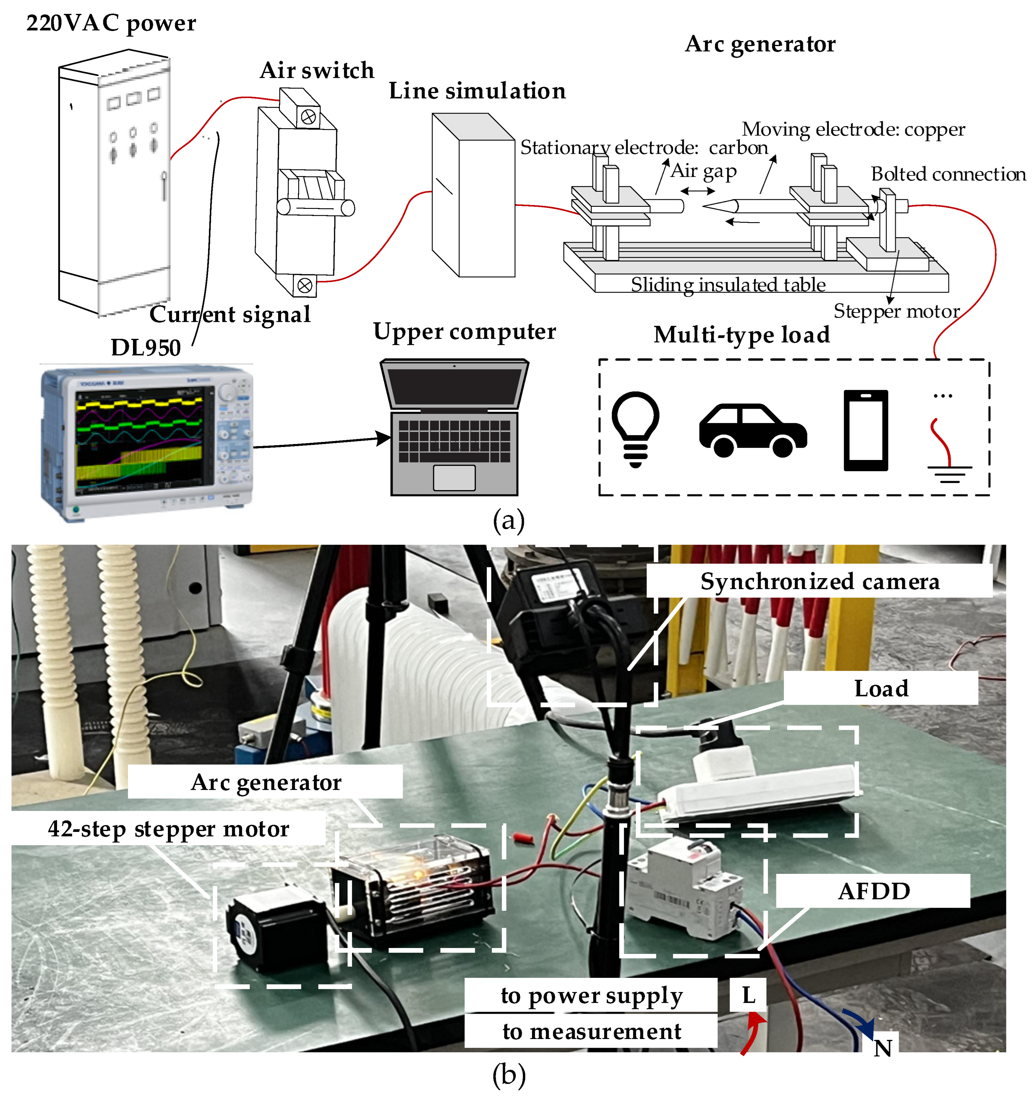
The experimental platform is built according to UL1699-2011 [33] and GB14287.4 [34] standards, and typical load types are selected to measure the experimental data under normal operating conditions and arc fault conditions. The experimental platform is powered by a 220 V residential circuit, and the wires are connected by BVR national standard multi-stranded soft copper wires with a cross-section of 4.0 mm2, in which overcurrent and leakage protection devices are strung to protect the rated current of 16 A. The arc generator consists of bolt-controlled sliding copper electrodes and static graphite electrodes, which are separated from each other in order to stimulate the series arc. The carbon electrode is chosen because it has a very high melting point and sublimation temperature, which effectively prevents the electrodes from fusing together during arcing. This is crucial for ensuring that the arc can extinguish and re-ignite consistently across multiple AC cycles, thereby generating a stable and repeatable series arc fault signature for measurement. The gap length is controlled by a servomotor communicating with RS485 protocol; in addition, a miniature circuit breaker with arc protection function is connected in series in the circuit. This miniature circuit breaker is a Siemens 5SM6011-2, manufactured in Beijing, China. Throughout the entire process, the protective switch did not activate. The wiring diagram of the experimental platform is shown in Figure 3.

3.1.2. Arc Fault Current Measurement

The HCPX8030 AC/DC high-frequency current probe was used to collect the main line current signal, its bandwidth (−3 dB) distribution from DC to 50 MHz, range 0–30 A, connected to YOKOGAWA DL950 oscilloscope to observe the current waveforms collected, the sampling rate was selected as 200 kHz, DC coupling mode, where the probe ratio is 10:1. According to UL1699- 2011 and GB14287.4, typical load types were selected to measure the single load experimental data under the operating conditions and arc fault conditions. Typical load types 2011 and GB14287.4, considering photovoltaic and battery cells in the Chinese market, were selected to measure single-load experimental data under normal operating conditions and arc fault conditions. The load types are cover resistive and resistive–inductive; switching appliances are converted to DC power by AC/DC rectifiers, and measured loads are categorized into two types according to whether the wiring contains an adapter or not.
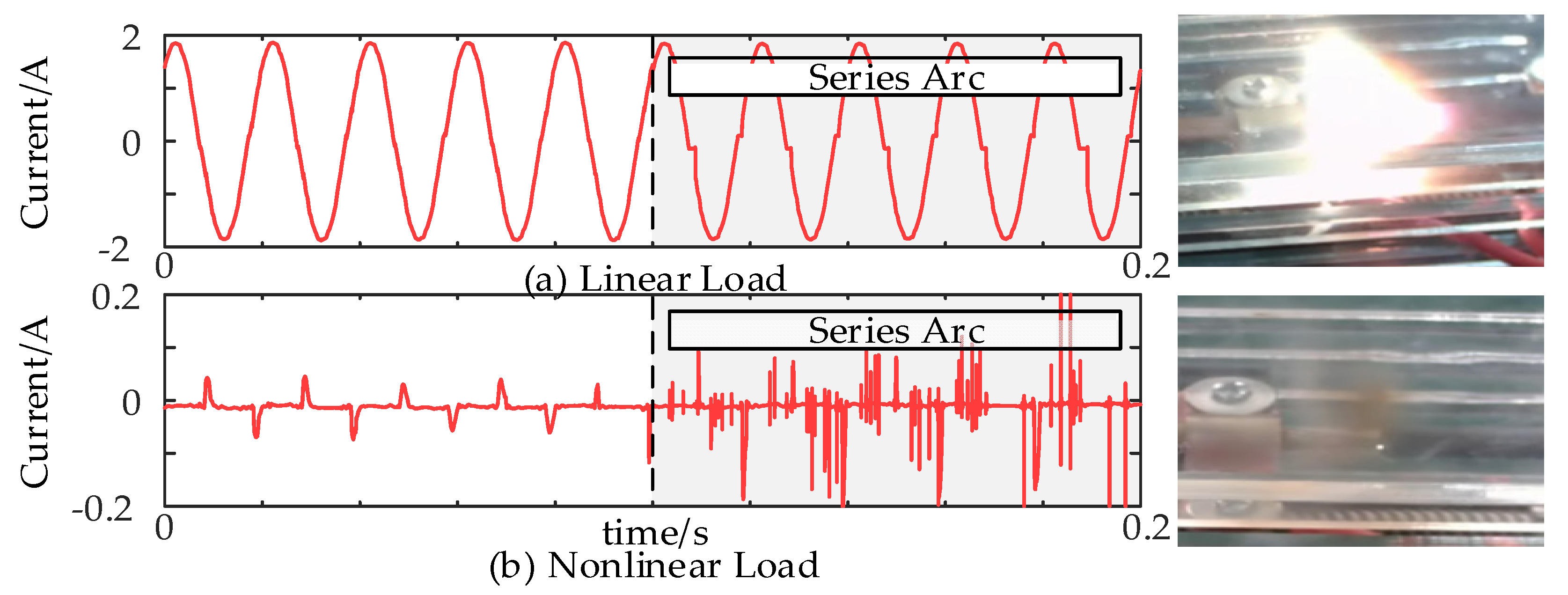
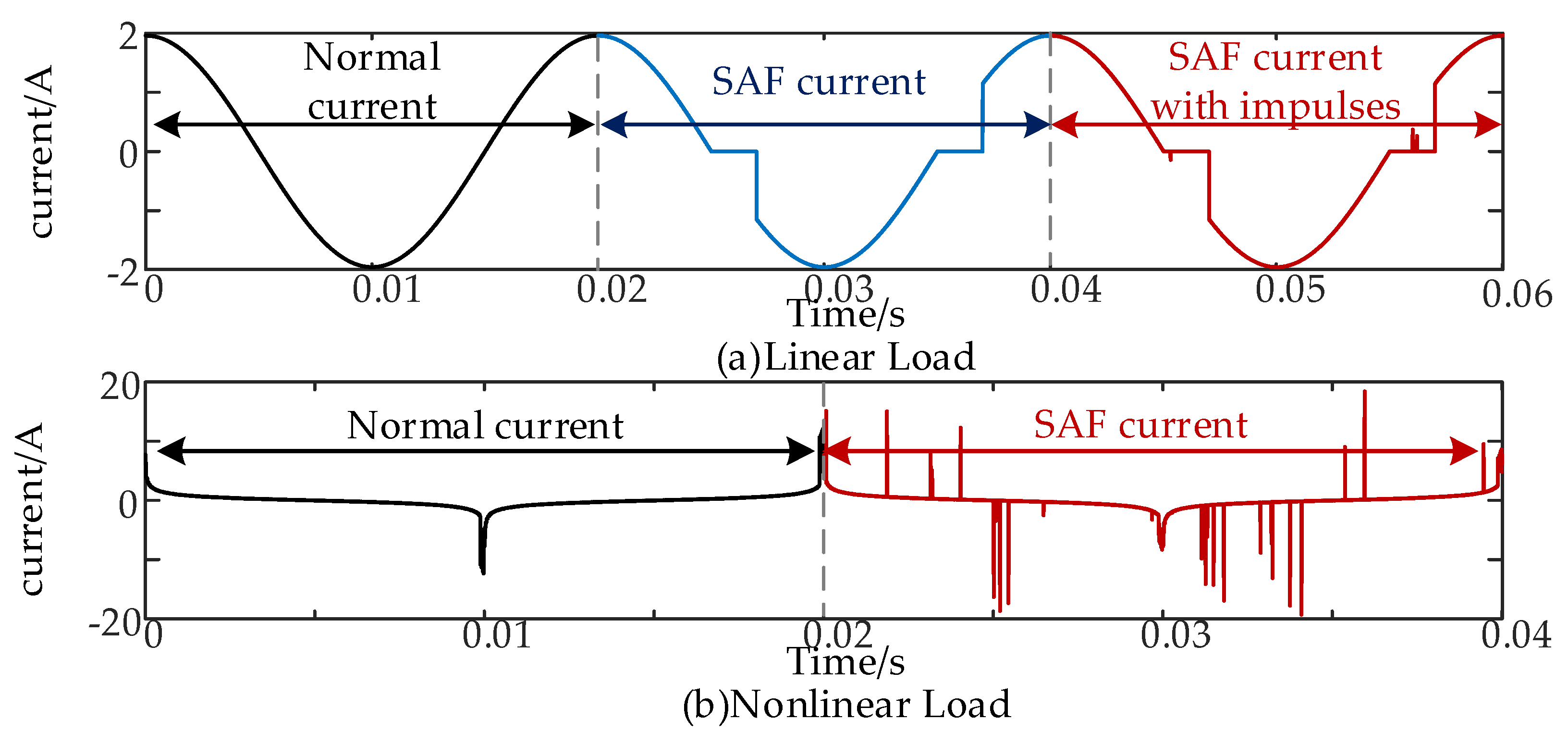
The power sizes of the selected loads span from tens of W to thousands of W to cover typical working conditions with different power sizes. The current waveforms of the above loads are measured and characterized in both time and frequency domains to construct a knowledge map of the normal waveforms of users’ electricity consumption under different load conditions. Repeat the experiment to take 10 samples of periodic waveform data under the normal state of each load, and obtain its time domain waveform and frequency domain spectrum. Figure 4 shows the measured current conditions with arc patterns for both loads. In the time domain, the linear load still retains a more obvious sinusoidal characteristic; nonlinear loads do not have obvious sinusoidal characteristics, which manifests itself as a positive and negative frequency cycle pulse, governed by thyristor conduction control logic. The different nonlinear load pulses of the rising speed and falling speed are different for different nonlinear loads. In addition, even if the two loads share the same adapter, the current waveform form also has obvious differences, as the switching power supply load current type is diverse; it is difficult to rely on an exhaustive way to list them completely.
In the frequency domain, the set sampling rate of 200 kHz captures the frequency domain features below 100 kHz. The linear load harmonic content is small, dominated by the industrial frequency fundamental content, and the total harmonic distortion rate does not exceed 30%. The harmonic components of nonlinear loads account for a large proportion, of which 10 kHz, 20 kHz, 30 kHz, and 65 kHz are the main ones, but the specific proportion varies with the load type, and it is difficult to find a uniform law to characterize the harmonic content under different loads; from the time–frequency perspective, the signals of linear loads are basically unchanged in the full-frequency band, with the amplitude nearly unchanged and the frequency remaining stable, and the low-frequency band of nonlinear loads also basically unchanged, with the amplitude and frequency nearly unchanged, and the frequency nearly unchanged. The low-frequency band of the nonlinear load is basically unchanged; the amplitude and frequency are approximately the same, but the high-frequency band fluctuates (10 kHz, 20 kHz, 65 kHz), and the amplitude rises significantly when the pulse spike occurs in the current, but then stabilizes after the pulse spike is over.
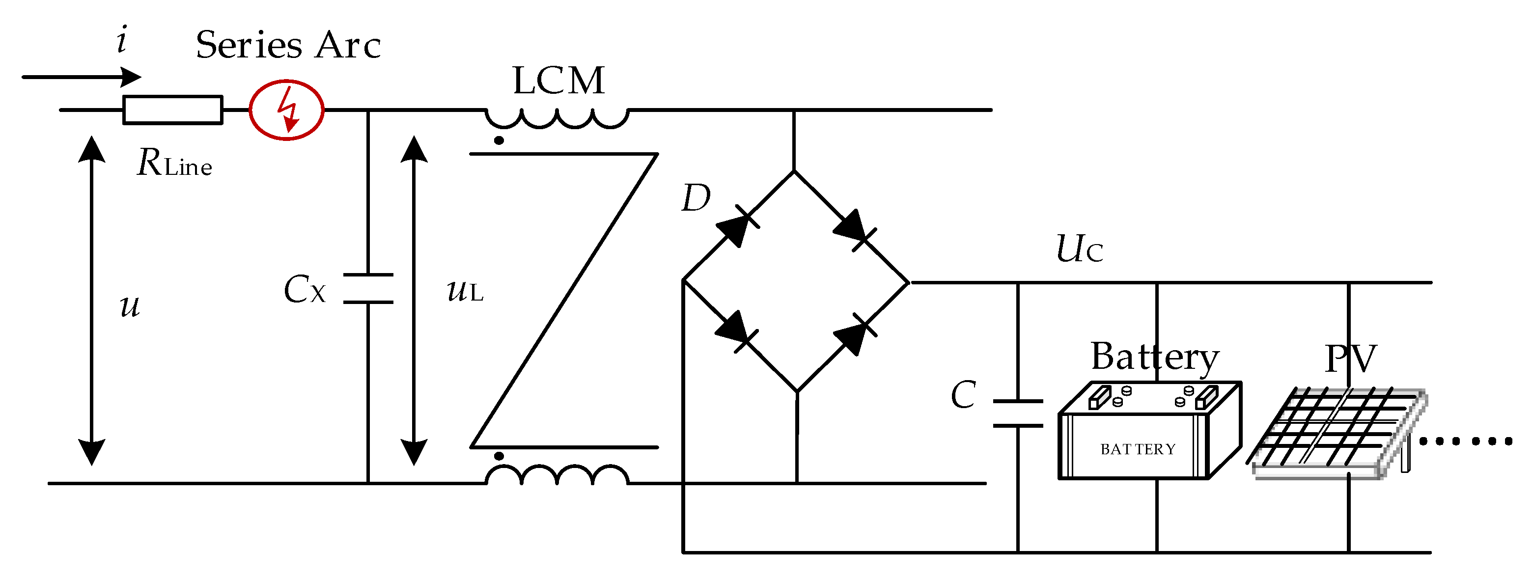
Modern grid-tied inverters are controlled to act as high-quality current sources, injecting a near-sinusoidal current into the grid with very low total harmonic distortion (THD). Consequently, under normal operation, the current waveform contributed by an inverter is comparable to that of a high-power-factor linear load. The linear load’s normal operation of the current shows obvious sinusoidal characteristics, where the occurrence of series arc faults can be observed when the obvious asymmetry is of the flat shoulder zero-rest phenomenon; the nonlinear load input stage generally consists of an electromagnetic interference EMI filtering circuit and a rectifier circuit, as shown in Figure 5, the input alternating current flows into a smoother DC output, and the output side of the back stage circuit can then be defaulted to a resistor. LCM is a common-mode choke used to eliminate the electromagnetic interference, which leads to its normal operating conditions also having a long zero-rest time, due to the small capacity of capacitor Cx causing the current to quickly reignite and extinguish from zero. Electromagnetic interference, which leads to its normal operating conditions, also has a long zero-rest time, and the occurrence of the series arc, due to the small capacitance Cx, leads to the arc quickly rekindled and extinguished; the current increases from zero and quickly returns to 0, indicative of the pulse form performance.
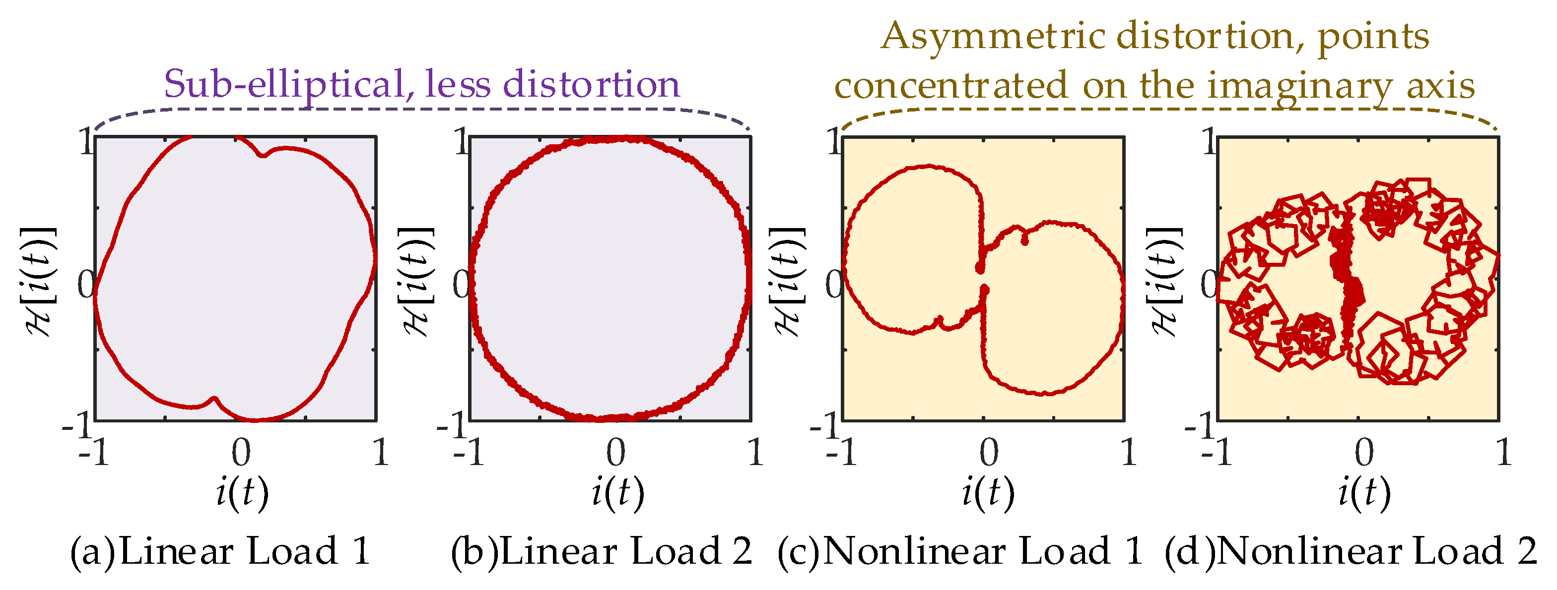
Further, the GLT image of the measured normal operating current signal is plotted according to Section 2, as shown in Figure 6. Because the normal operating current of the linear load is close to sinusoidal waveform, its GLT image shows a nearly elliptical shape, and its small amount of harmonic content makes its GLT image have few more-than-one-ellipse “crackle” phenomena; the normal operating current of the nonlinear load, due to the control of the thyristor and the other control, and the zero-rest time in the whole cycle account for a large percentage of a large number of sample points fall on the imaginary axis of the GLT image, in addition to being due to the increase in the proportion of high-frequency harmonics. The normal operating current of the nonlinear load is controlled by the thyristor and so on, and a large number of sampling points fall on the imaginary axis of the GLT image, reflecting the obvious “8” shape due to the increase in the proportion of high-frequency harmonics.
The arc generator is controlled to produce a stable arc, the load type currents are measured for different load cases, and their GLT images are plotted. As shown in Figure 7, (a) shows the comparison of current and GLT image between linear loads with series arc faults and normal operation, and, due to the arc zero-rest phenomenon, an obvious curvature mutation and elliptical trajectory breakage can be observed in the GLT image, whereas (b) shows the comparison of image between nonlinear loads with series arc faults and normal operation due to the large number of random impulses caused by arcs introducing a large number of high-frequency components, and the GLT image superimposes a large number of triangular closed enclosures. Through the GLT image, the one-dimensional time series of the current is mapped into the trajectory image of the two-dimensional complex plane, and the low-dimensional fault features are transformed into the topological expression of the high-dimensional space, which effectively amplifies the fault features.

3.2. Modeling of Measured Fault Current

3.2.1. Analytical Mathematical Modeling of Two Different Types of Load Currents

A linear sinusoidal current is observed during normal operation of common linear loads. The current for normal operation of both loads under ideal power conditions is expressed by Equation (2):
i nor = α n = 0 , 1 , 3 , 5 N cos n ( ω t + φ ) n β
where α is the current amplitude coefficient, determined by the power size, N is the number of harmonics counted, ω = 2 π f , and β is the harmonic component attenuation factor, where, generally, β > 2 in the case of linear loads, and β < 1 in the case of nonlinear loads.
When series arcing faults occur, different fault characteristics are superimposed, and the fault characteristics of linear loads are controlled by the zero-rest moments of thermal inertia, as well as random pulses, which are represented by Equation (3):
i abn = i nor + i pause + i thermal + i pulse i pause = i nor × u ( t t 0 t thermal ) u ( t t 0 t thermal + Δ t ) i thermal = i nor × u ( t t 0 t thermal ) u ( t t 0 t thermal + Δ t ) × δ ( t t 0 t thermal ) i pulse = j = 0 C N j × sgn ( r a d n ) × δ ( t τ p )
where t0 denotes the zero break moment of each cycle, u(t) is the step function, Δ t is the zero break length, tthermal is the compensation moment considering thermal inertia, C is the number of random pulses, Nj is the pulse amplitude, sgn is the pulse polarity, δ is the unit impulse function, and τ p is the random moment of the impulses during zero break phase.
The fault current of a nonlinear load consists of two components: the normal operating current and the random pulse current. The zero-rest phenomenon of the nonlinear load is submerged in its normal operation of the switching tube conduction control, and the main fault characteristics are reflected in the polarity of the same phase as the voltage of the obvious random pulse spikes, expressed by Equation (4):
i a b n = i nor + i pulse i pulse = M × k = 0 sgn ( i a b n ) × δ ( t k π ω φ + Δ t ) + j = 0 C N j × sgn ( v ( t ) ) × δ ( t τ j )
where C is the number of random pulses, Nj is the random pulse amplitude, v(t) is the instantaneous value of the supply voltage, and τ j is the moment of occurrence of the random pulse, conforming to the Poisson distribution τ j P ( λ ) . The current case for two types of numerical model reconstruction is shown in Figure 8, where (Figure 8a) α = 1 and β = 8, Nj = 0.5, C = 20; Figure 8b illustrates that α = 1, β = 0.8, M = 50, and C = 20.
The key insight is that the defining characteristics of a series arc fault—such as the current zero-break phenomenon and the random high-frequency pulses caused by the inherent instability of the arc column—are physical phenomena governed by the fault itself and the connected load. These features directly modulate the load current, regardless of whether the energy is sourced from the grid or an inverter. Since our GLT transformation and subsequent models are built upon analyzing the morphology of the current signal, they are inherently sensitive to these specific modulations. The “background” current, being sinusoidal and stable from the inverter, does not obscure but rather provides a clean carrier upon which the arc fault imposes its distinctive signature. Therefore, the proposed numerical models for both linear and nonlinear loads comprehensively cover the dominant SAF features observed on the AC main, making the method robust in systems with integrated PV and battery storage. The following simple parameter optimization algorithm is designed to verify the feasibility of the proposed model to reflect the real data.

3.2.2. Particle Swarm Optimization to Verify Model Universality

Considering the stochastic nature of the actual arc signal, it is difficult to select a particular observation period as the reference system to verify the applicability of the proposed model, and it is also difficult to compare the similarity between the proposed numerical model and the observed fault current according to a certain index cluster. Therefore, the particle swarm algorithm is used to find the optimal parameters automatically, and the observed fault current signal is used as the optimal solution, and the initial random parameters are given to observe whether the proposed numerical model is close to the observed fault signal in a limited number of iteration steps, which is the basis for evaluating the general applicability of the proposed model. The PSO algorithm starts from a stochastic solution, tracking the extremes of each individual in each iteration and transferring their information to each other to quickly converge to the optimal solution.
Normalization of all current signals eliminates the effects of parameters such as α , M, etc. In conjunction with Section 3.2.1, the series arc current of a linear load can be represented by a numerical model with adjustable parameters of zero-rest time, arc thermal inertia magnitude, and pulse intensity. The initial velocity and position of each particle of a linear load can be expressed by Equation (5):
V i ( 0 ) = Δ t pause 1 , Δ t pause 2 , Δ i thermal 1 , Δ i thermal 2 , Δ N pulse X i ( 0 ) = t pause 1 , t pause 2 , i thermal 1 , i thermal 2 , N pulse
The nonlinear loaded series arc fault signal is dominated by a very strong pulsed current, and its corresponding initialized particle’s velocity and initial position can be expressed by Equation (6):
V i ( 0 ) = Δ N pulse , Δ M pulse X i ( 0 ) = N pulse , M pulse
At k + 1 iterations, the velocity and position of particle i are updated according to Equation (7):
X i ( k + 1 ) = X i ( k ) + V i ( k + 1 ) V i ( k + 1 ) = ϖ V i ( k ) + c 1 r 1 ( p b i ( k ) X i ( k ) ) + c 2 r 2 ( g b i ( k ) X i ( k ) )
where i represents the i-th particle in the total particle population, ϖ is the inertia weight that keeps decreasing in each iteration to avoid the iterative process from falling into the local optimum, c1 and c2 are the acceleration coefficients, r1 and r2 are the random numbers between (0, 1), and pb and gb are the positions of the individual extremes and the global extremes. The PSO algorithm is implemented in a Matlab R2023a environment to take the actual observed series arc fault current waveform as the global optimum, initialize the fault current parameter particle swarm to participate in the global search, and adjust the optimization direction of PSO with the sum of squares due to error (SSE) as the objective function to obtain the closest model parameters by gradual iteration.
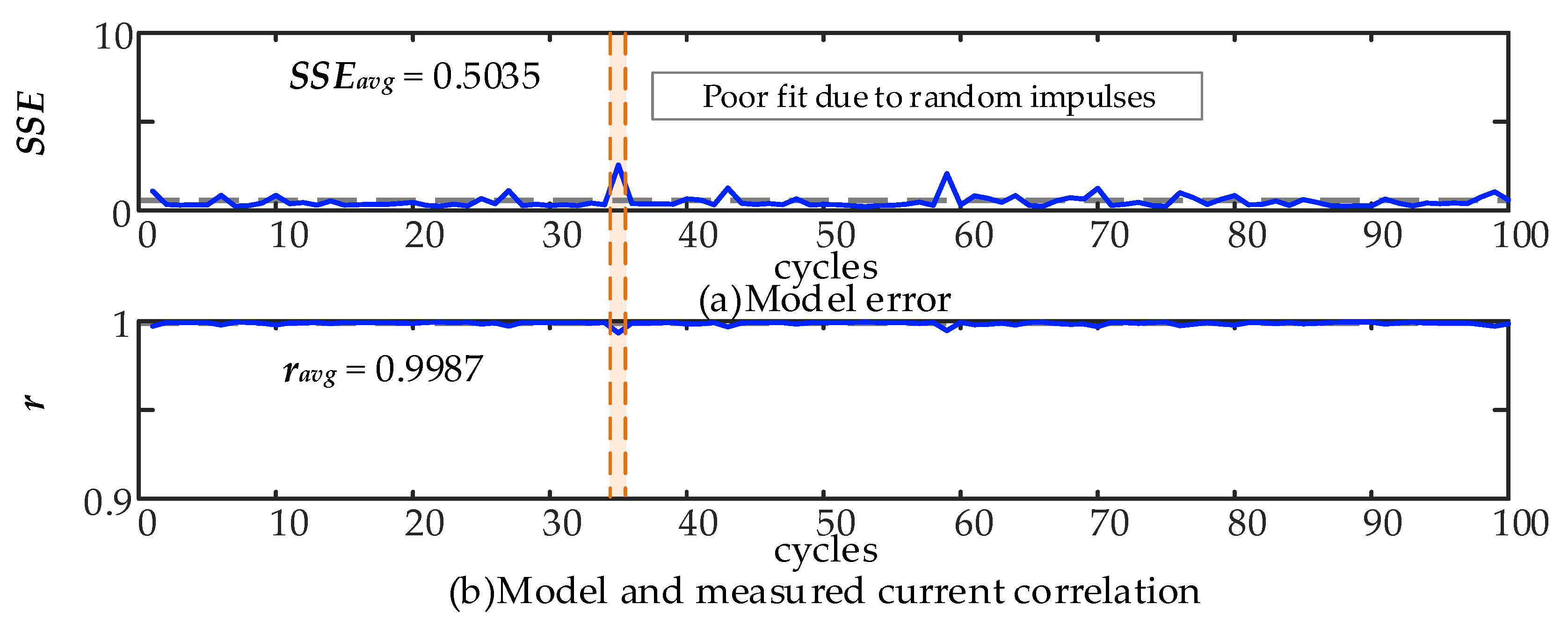
The performance results of the proposed model under the PSO algorithm optimization are shown in Figure 9. Figure 9a shows the performance of the current under linear load mode, where the model fits the zero-break characteristics of the arc well and responds to the random impulses during the zero pause; Figure 9b shows the performance of the current under nonlinear load, which, despite the discounted effect compared to the linear load case, still responds positively to the large number of random impulses embedded in the measured signals. The current performance under a nonlinear load is shown in b. Although the effect is discounted compared to the linear load case, it still responds positively to the large number of random pulses embedded in the measured signal. It can be expected that when the number of iterations is increased, the fitting effect of the nonlinear load model can be effectively improved. However, due to the stochastic nature of series arc faults with nonlinear SW loads, accurate reconstruction for a single-cycle signal is not very meaningful. Figure 10 shows the SSE and r values based on 100 measured arcs containing complete cycle data using the PSO algorithm, and the results show that the average error is 0.5035, and the average correlation coefficient reaches 0.9987, which reflects the good generalization and accuracy of the proposed numerical model.

4. Proposed SAF-GLT Learning Methods

4.1. Sample Generation and Model Training

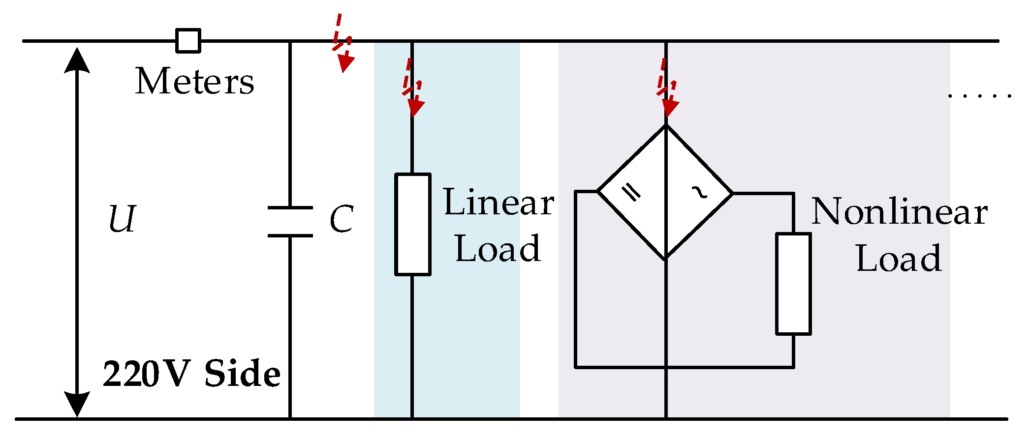
The circuit is shown in Figure 11. It is a typical low-voltage consumer’s electricity circuit. The trunk line is fitted with a smart meter with a wave recording function. Neglecting line impedance parameters, SAF occurs in the trunk or branch circuit. The branch circuit is connected to two adjustable loads, controlling their load types to measure different main circuit currents. At the same time, simulating the trunk circuit generates SAF, and the branch circuit separately generates SAF to complete the sample database.
In the process of generating the samples, different combinations of load types are considered, e.g., different combinations of power sizes, different zero-break durations, different pulse intensities, and also different initial phase angles of the faults. Different proportions of noise are superimposed, and the specific meanings of the parameters can be found in Section 3, as shown in Table 2:
Normal and abnormal current signals are generated in a Matlab environment according to the above parameter settings, and the corresponding GLTs are plotted, converted into grayscale maps, and batch-saved in png format; the pixel size is set to 224 × 224 to obtain the image dataset of the GLTs oriented to series arcs.

4.2. Load Modal Identification via K-Means Algorithm

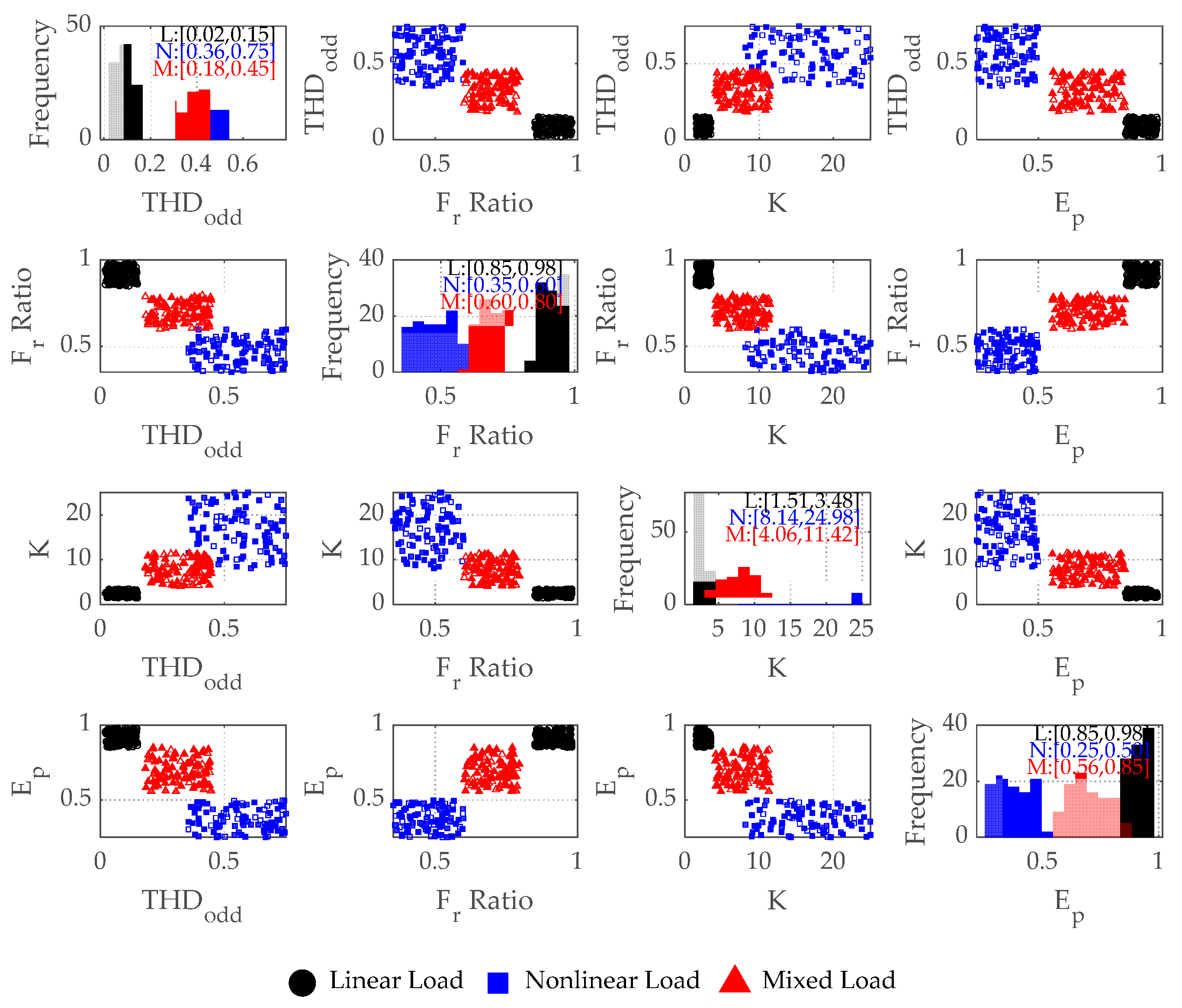
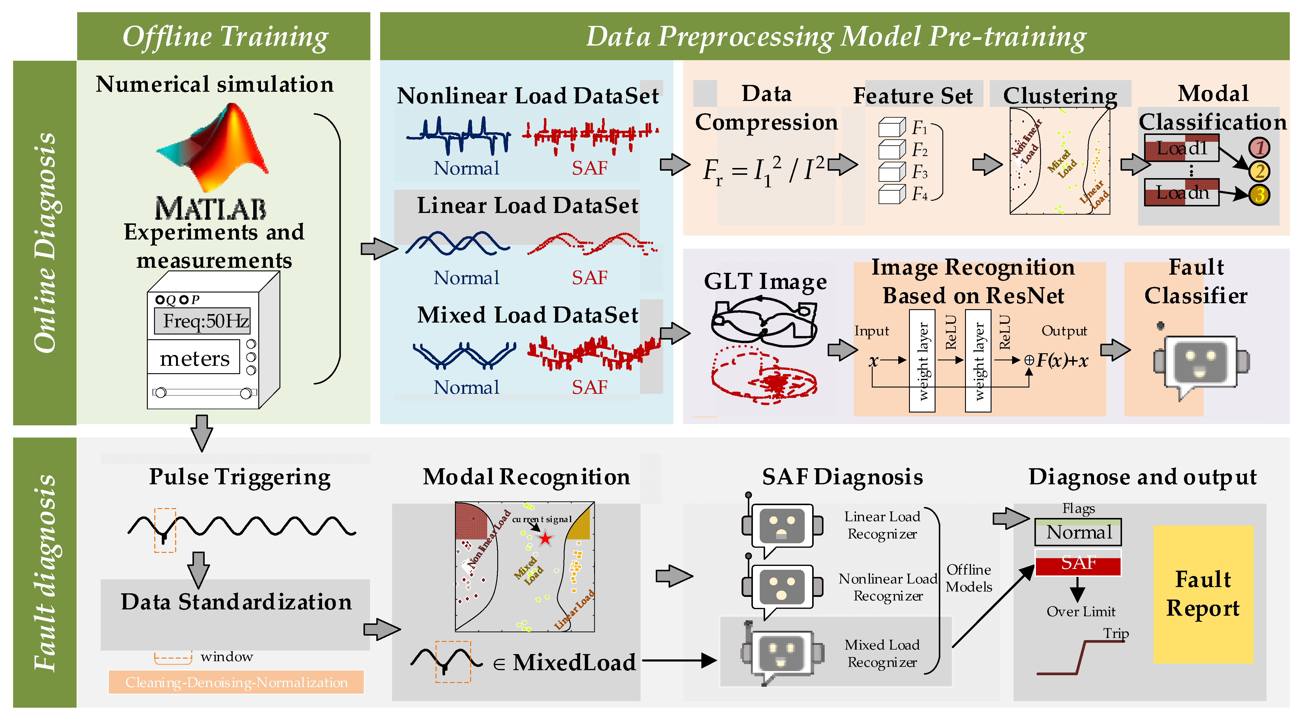
Compared to the training set that contains both linear and nonlinear load trajectories, the classifier’s performance in terms of recognition accuracy is better when there is only one type of load in the training set [35,36]. Based on this premise, feature engineering is designed as a preprocessing step of the algorithm: the K-means algorithm is based on the modal identification of the load type, and the output load type is identified by a specific pre-trained classifier for the next fault identification step. The specific feature engineering is selected in Table 3.
Sliding computation of the feature vector with a sliding step of 20 ms (one cycle), input current signal for feature extraction, and Z-score dimensionless normalization are evaluated. Furthermore, based on K-means clustering, logical decision labeling is output. The classification situation and decision boundary delineation based on the sample database are shown in Figure 12. At the same time, five consecutive windows are set to determine the same mode before switching the model to prevent model jitter. The computational complexity of the proposed method is O(NlogN) + O(N).

4.3. Complete SAF-GLT Image-Based Detection Algorithm

As illustrated in Figure 13, the proposed SAF-GLT image-based detection algorithm has been derived from a standard electricity circuit for a low-voltage customer, taking into account the PV and battery storage. Based on the mathematical analytical model in Section 2, and considering different load types, power sizes, zero-break moments, and time durations, as well as simulating different signal-to-noise ratios, the sample set of the training validation set is batch generated in the Matlab environment, and the image recognition classification task is carried out in the Python 3.11 environment after pre-processing steps such as cleaning and screening. The ResNet50 model was selected [37]. A total of 30,000 samples were selected at random from normal operation and series arc faults. These samples were then divided into training and validation sets at a ratio of 8:2. The batch size is set to 20, the initial learning rate is 0.01, the learning rate decline rate is 0.9, the Adam optimizer is selected to train the final fully connected layer, and the number of iterations is set to 100. Accuracy (Acc), precision (Pre), recall (Recall), and F1 score are chosen for model precision evaluation as follows (8):
A cc = T P + T N T P + T N + F P + F N P re = T P T P + F P R ecall = T P T P + F N F 1 = 2 P re R ecall P re + R ecall
where TP, TN, FP, and FN represent the number of positive and negative samples with correct predictions and the number of positive and negative samples with incorrect predictions, respectively. Targeted normal and abnormal arc fault condition identification tasks are carried out for each load type.
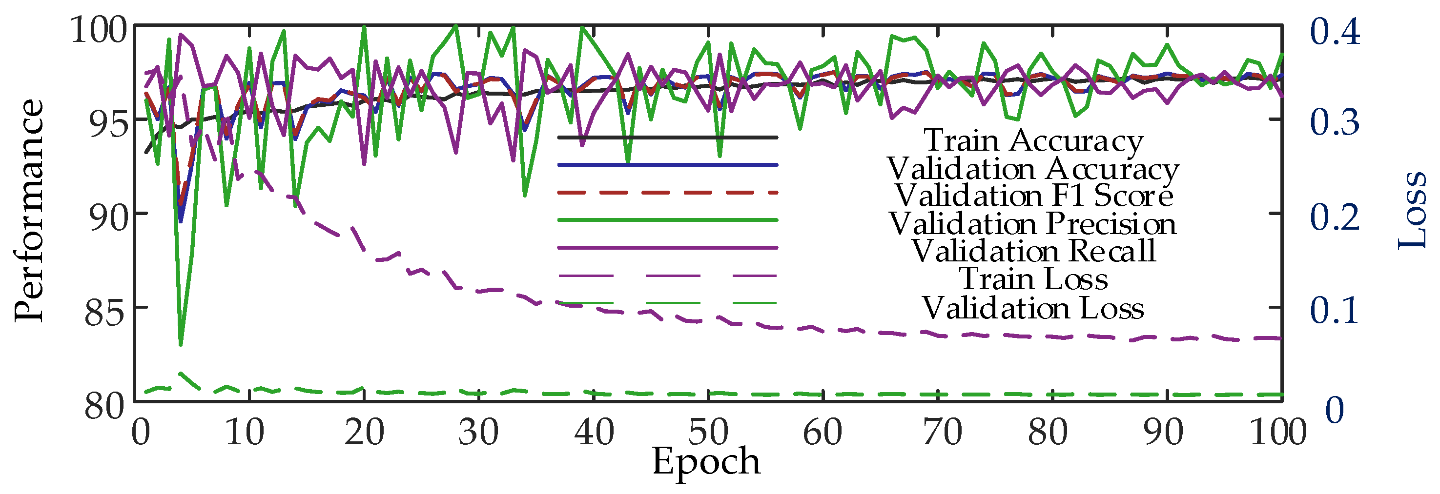
Figure 14, Figure 15 and Figure 16 show the training results of the GLT samples for different types of loads. In the linear load sample, training for a validation accuracy of 99% and a training accuracy of 98% are achieved in the initial iteration, and after 100 iterations, the learning rate decreases from 1 × 10⁻² to 5 × 10⁻⁵, and a validation accuracy of 99.91% and a training accuracy of 99.83% are achieved, with a precision rate of 99.95%; the recall rate reaches 99.88%, and the F1 score reaches 99.92%; in the training of nonlinear loaded samples in the initial iteration, we achieve 97% validation accuracy and 94% training accuracy, and after 100 iterations, the learning rate decreases from 1 × 10⁻² to 5 × 10⁻⁵, and finally achieves 98.93% validation accuracy and 98.13% training accuracy, where the precision rate reaches 98.72%, recall rate reaches 99.15%, and the F1 score reaches 98.94%; after 100 iterations in the training of mixed-loaded samples, the validation accuracy of 97.33% is finally achieved with 97.11% training accuracy, validation precision of 98.43%, recall rate of 96.22%, and an F1 score of 97.31%, which demonstrates a slight decrease in the accuracy compared to the previous two cases. All results are shown in Table 4.
An efficient and accurate series arc detection algorithm based on operating mode recognition determines the current load type of electricity consumption by monitoring the current harmonic content of the electricity circuit, and effectively identifies series arc faults based on offline classifiers under different load types; the algorithm relies on the startup of the abnormal current impulse [38]: when the impulse coefficient of three consecutive cycles is detected to be greater than the ratio of impulse coefficient product of the normal operating situation, or is greater than 8, the algorithm starts. The pulse coefficient is defined as λ j = i j / 1 3 [ j = i 5 i i max ( i i ) min ( i i ) ] . After the startup, read a cycle of the current sequence to calculate the fast Fourier transform, calculate the energy ratio of different frequency bands for load modal discrimination, and output the type of operating conditions. It is also based on the following: the introduction of the previous section to obtain the GLT grayscale map, the load modal input to the corresponding offline pre-training network diagnosis, and the diagnostic results of the output fault trip signal to drive the circuit breaker action. The validation of the algorithm is based on simulation data, which covers the situation described in the previous section. In this paper, the normal pulse coefficient is taken in the algorithm, and the experimental environment adopts a 2.50 GHz Intel i5-12400F CPU, 16 GB RAM, and NVIDIA RTX 4060Ti GPU, and the specific method identification results are shown in Table 5, Table 6 and Table 7.
It is noted that under mixed load conditions, the final accuracy achieved was only 87.42%, significantly lower than that observed under single load mode types. The primary cause of the accuracy drop is not the inherent capability of the GLT image recognition model itself, but rather the error propagation within the multi-stage pipeline, specifically from the preliminary load modal identification step. For example, a significant portion of mixed-load samples is misclassified as either “linear” or “nonlinear” load types. This initial misclassification is catastrophic for the subsequent step. A mixed-load sample with a series arc fault (SAF), if misclassified as a “linear” load, is then fed into the linear load ResNet classifier. This classifier, trained exclusively on pure linear load patterns, is highly likely to misinterpret the hybrid features and produce an incorrect output (e.g., classifying a faulty mixed-load sample as “normal”). This error propagation directly leads to a drop in overall accuracy to 87.42%. This indicates that the current mode recognition module based on K-means clustering relies on simple feature vectors, struggling to perfectly separate these mixed features. To address the aforementioned issues, future research will focus on developing more sophisticated and robust modal identification modules, specifically including exploring broader time–frequency feature sets and replacing the K-means algorithm with lightweight supervised classifiers specifically trained to distinguish linear, nonlinear, and mixed load characteristics.

5. Implementation Assessment and Method Analysis

This section will discuss the optimization of the experimental conduct and data portion of the proposed method, while the experimental control and ablation experiments will be conducted and compared to other methods. Finally, we point out the gap between the current method and its practical application, as well as the direction for future work.

5.1. Sample Rate Sensitivity Analysis

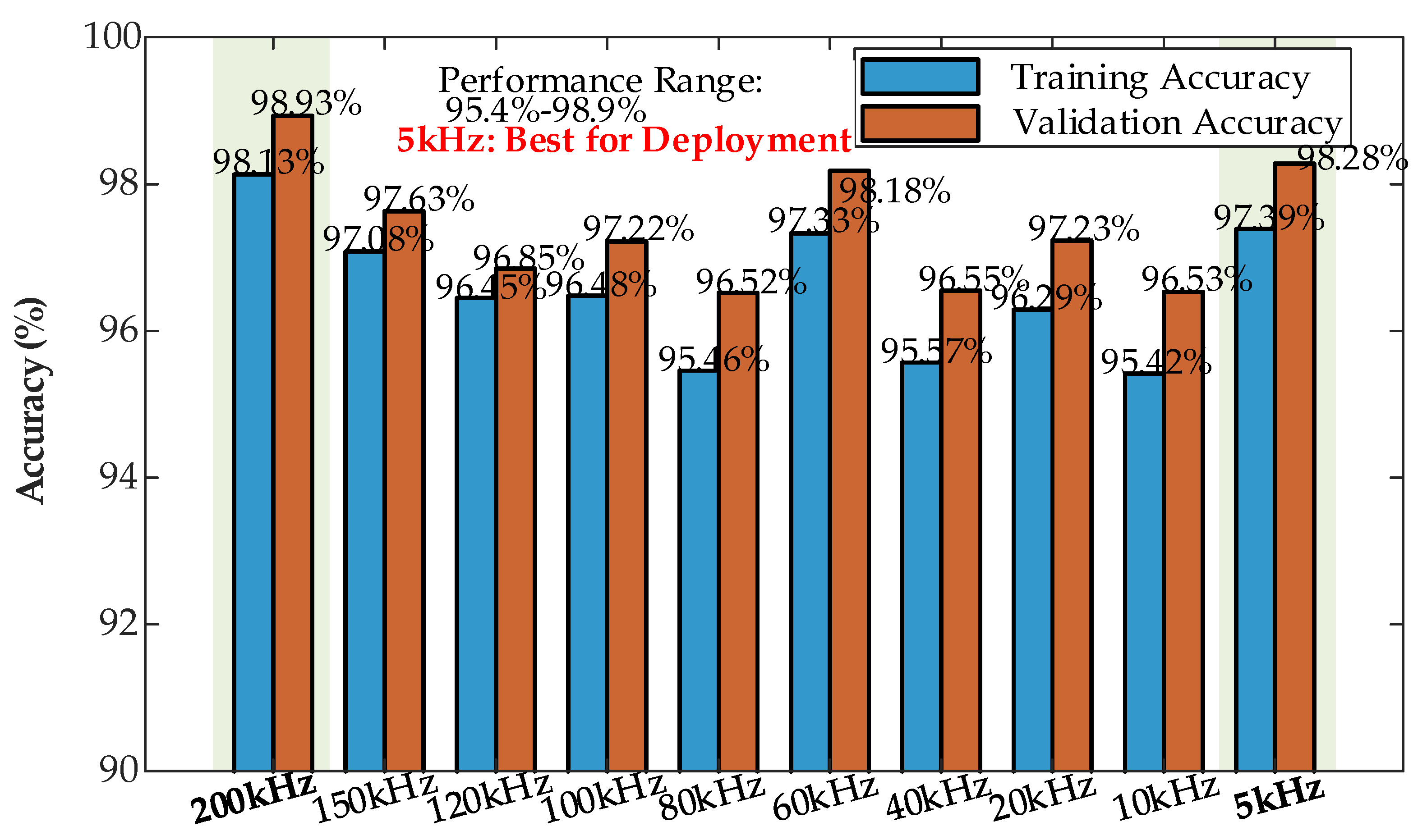
In accordance with the 200 kHz sampling rate experiment previously conducted, the subsequent steps of the experiment are to be repeated by means of downsampling to 10 kHz. This will facilitate the evaluation of the model’s performance at varying sampling rates, thereby enabling the determination of the optimal sampling rate. This optimal rate will take into account both accuracy and hardware cost. The experimental results are shown in Figure 17. The highlighted background color indicates the experimental group with better results.
The results show that the method proposed in this paper is barely affected by the sampling rate. This may be caused by the high sampling rate introducing high-frequency components that the fitness model cannot cope with. A low sampling rate does not significantly reduce the model accuracy, but at the same time, a low sampling rate relaxes the algorithm’s need for acquisition devices and algorithm configurations, and a sampling rate of 5 kHz (about 128 points per cycle) can already satisfy the actual engineering needs.

5.2. Image Quality Compression Experiment Analysis

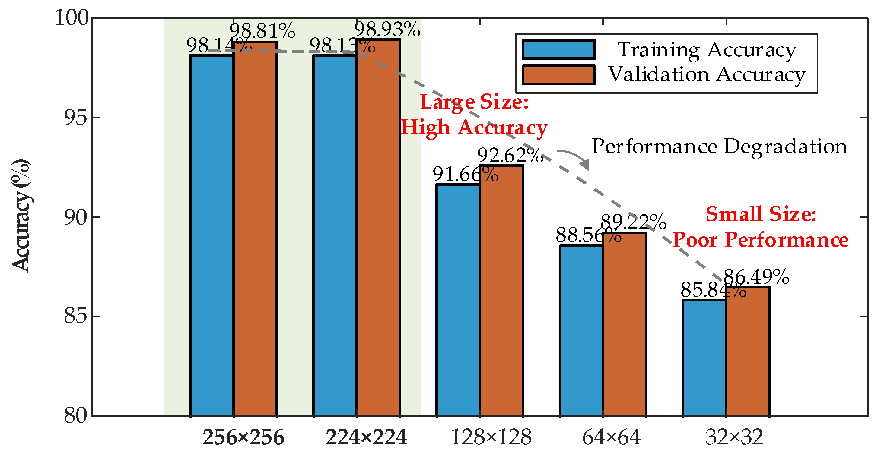
As demonstrated in the preceding experiments, a PNG image of GLT size 224 × 224 with a point size of 224 × 224 was generated. PNG images with different specifications of different resolution sizes are now generated to quantify the effect of image quality on the classification performance of the classifier in an attempt to find the quality threshold of acceptable images. The experimental results are shown in Figure 18.
A total of four image sets, 32 × 32, 64 × 64, 128 × 128, and 256 × 256, are generated. The results indicate a positive correlation between image size and model accuracy within a certain range. It is evident that increasing the image size leads to enhanced texture details, closer alignment with the context, and improved suitability for the classifier in capturing dynamic features. However, when the image size is reduced, some discriminative features become blurred or even disappear, thereby affecting the classification efficacy. Furthermore, while increasing the size to a certain extent does not significantly enhance the classification performance, it can substantially increase the computational overhead. Consequently, selecting an image size that is neither too small nor too large can optimize the balance between algorithmic accuracy and computational efficiency. The highlighted background color indicates the experimental group with better results.

5.3. Trajectory Characterization Methods Comparison

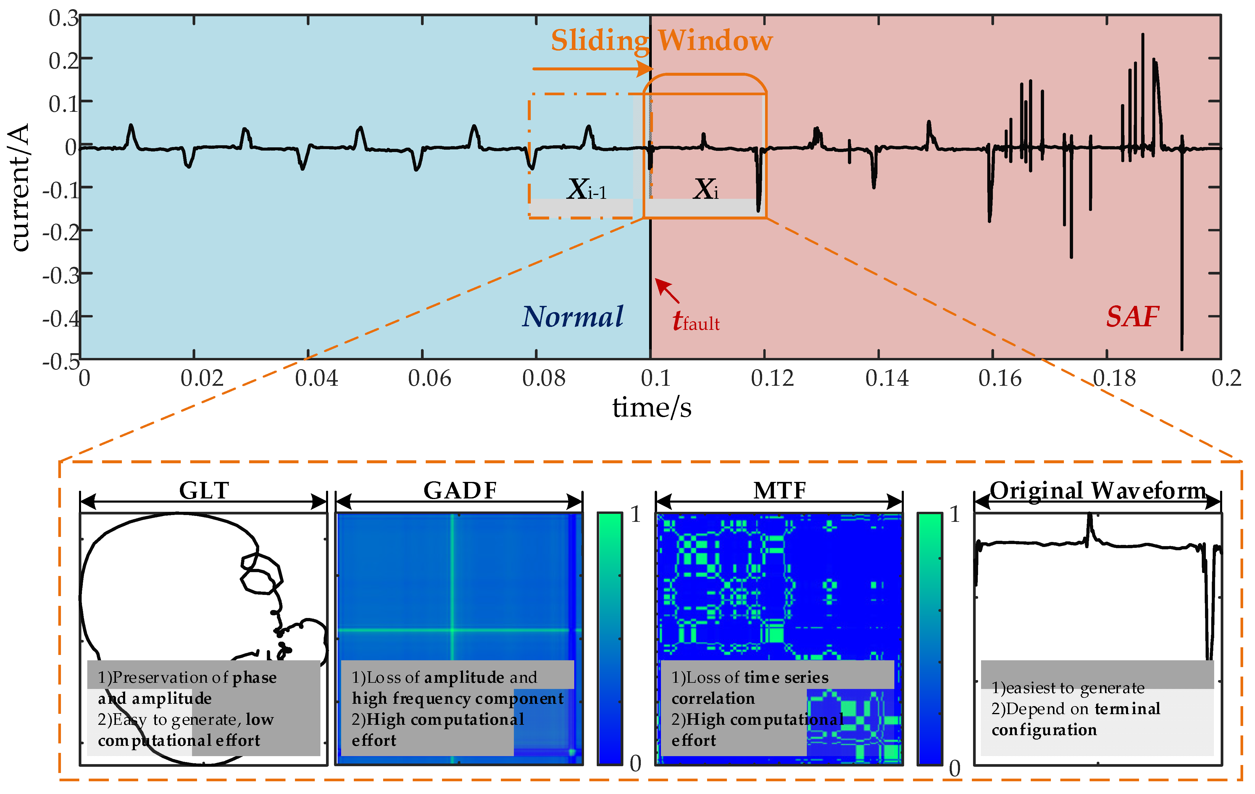
In recent years, the measured voltage–current volt–ampere characteristic curves have been used for high resistance fault detection. As the application of image recognition technology in the field of power systems continues to expand, there have been a variety of methods such as the use of fused waveform images for direct recognition, converted to Gramian angle field, Markov’s migrated field, and so on, in order to prove that the advantages of the GLT for the amplification of the capture of the characteristics of the series arc faults (such as the zero-break and impulse) as proposed herein. And to compare the accuracy as well as the computational complexity, the image sets of the Markov migration field as well as the Gram angle field are generated on the same dataset (nonlinear load case). Also, comparison experiments based directly on waveform images were carried out. The specific generation method is shown in the following equation:
GADF is a coding technique that realizes the change in a time series into a two-dimensional image using coordinate changes and the Gram matrix. The time series X = {x1, x2, …, xn} is measured and normalized according to Equation (9):
x ˜ i = 2 x i max X min X max X min X
Encoding the scaled time series in polar coordinates is carried out with the angular cosine, which corresponds to the radius of the timestamp, as in Equation (10):
θ i = arccos ( x ˜ i ) , 1 x ˜ i 1 , x ˜ i X ˜ r i = t i M
where ti is the timestamp corresponding to the sequence point xi and M is the normalization factor. After the above transformations, the time series has been reconstructed, and GADF A images can be further generated based on Equation (11):
A = sin ( θ 1 θ 1 ) sin ( θ 1 θ j ) sin ( θ i θ 1 ) sin ( θ i θ j )
MTF was first proposed by Wang Zhiguang et al. It has a close correlation with Markov chains and also keeps the information in the time domain. Assuming a time series X{t}, the data of the series are first divided into Q quartiles according to their value ranges, and any data point in the series corresponds to a unique qi (l < i < Q). Construct the Markov migration matrix W = (pi,j)Q×Q corresponding to the time series, where pi,j denotes the transfer probability of state i transitioning to state j with Σpi,j = 1. Consider the time information, and extend it to the MTF matrix M, as follows (12):
M = w i j | x 1 q i , x 1 q j w i j | x 1 q i , x n q j w i j | x n q i , x 1 q j w i j | x n q i , x n q j
where p k and p l denote the quantiles of x k and x l . Regarding W , it is probable that the quartile bucket it is located in is transferred to the other quartile bucket in which it is also located.
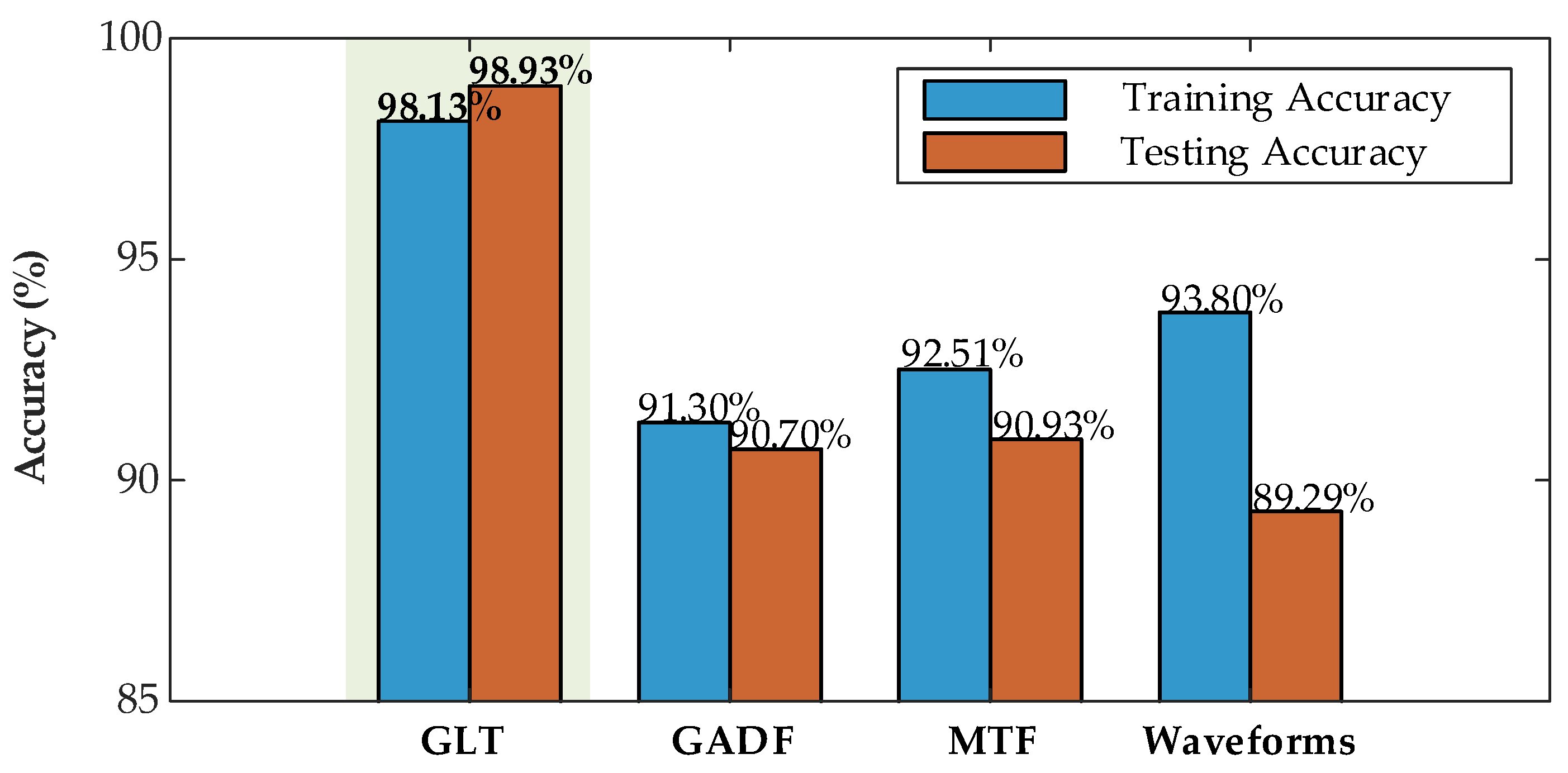
Incipient fault detection in reference [39] was performed using a GADF with an image size of 128 × 128. The results of the controlled experiments, taking into account the different size and sampling rate settings, are as follows: 82.55% validation accuracy and 81.87% training accuracy for the 128 × 128 image size at a 200 kHz sampling rate; 92.51% validation accuracy and 90.94% training accuracy for the 224 × 224 image size at a 200 kHz sampling rate; and 86.98% validation accuracy and 85.34% training accuracy for the 224 × 224 image size at a 5 kHz sampling rate. The GADF performs best at high sampling rates and high image sizes but is 5 percentage points lower than the method proposed in this paper. The size and resolution of a GADF image are limited by the length of the time series data; a time series that is too short does not provide enough information to generate an image. In addition, the GADF method loses amplitude information, the cosinization step does not capture high-frequency information well, and features such as harmonics and transients are corrupted; it is not suitable for series arc fault detection. The computational complexity of the GADF method, O(N2), also introduces an additional latency, which reduces the real-time performance of the method. Overall, GADF requires a high sampling rate to capture high-frequency features and is sensitive to image size, which makes it computationally demanding.
Under the same 224 × 224 image size, the same image recognition classifier background achieves 91.3% training accuracy with 90.7% validation accuracy, which is lower than that of the GLT method proposed in this paper, due to the loss of key arc features such as phase relationship/transient mutation in MTF and is caused by the complete preservation of Lissajous through geometrical projections. Since the MTF method is essentially a coding method based on probabilistic statistics, it loses the correlation of the time series, ignores the essential characteristics of the arc fault, and only retains the statistical distribution characteristics of the magnitude feature; when compared to the MTF method, the proposed GLT preserves critical phase relationships and transient signatures (e.g., zero-crossing distortion manifests as elliptical rupture). While MTF compresses temporal dynamics into probability transitions, the method’s O(N) complexity enables real-time processing at 200 kHz sampling, outperforming MTF’s O(N2) in embedded platforms.
Experiments on series arc fault identification based directly on waveform images have also been carried out [40]. But the method directly based on waveform image data recognition only retains the amplitude characteristics in the time domain, which makes the zero-rest phenomenon susceptible to being overwhelmed by noise. While those frequency domain methods, e.g., STFT makes it impossible to capture information like instantaneous frequency changes; all the harmonic components are compressed into the amplitude envelope, and a large amount of physical information is lost. In the normal operation of the linear load, the waveform image mainly reflects the sinusoidal characteristics, reacting to the GLT for the center of the circle in the round point of the ellipse; the zero-rest phenomenon is manifested as the amplitude to zero, reacting to the GLT for the ellipse trajectory to the y-axis tear. Sharp current pulses in the waveform image can be seen in a few samples where a sudden increase in the trajectory occurs, reacting to the GLT for the anomalies of a closed triangular enclosure. Under the 200 kHz sampling rate condition, the validation accuracy of the 224 × 224-sized image was 89.2%, and the training accuracy was 93.8%. This indicates that relying only on waveform image features cannot effectively extract image commonalities. In addition, from the point of view of algorithm complexity, the computational complexity of the preprocessing step of the waveform method revolves around O(N), and the computational complexity of the H-transform of the GLT also revolves around O(N), and the difference between them is negligible. The time to draw the two images in the deployed system is also approximately equal, but to achieve the same accuracy as the GLT method, a higher sampling rate and image size are required to capture more detailed fault information, or a deeper structured network is chosen. As illustrated in Figure 19, the schematic of the generation of the four different trajectory methods is demonstrated. A comparison of the four methods’ accuracy results is provided in Figure 20. The highlighted background color indicates the experimental group with better results. The characteristics of the different methods are summarized in Table 8.

5.4. Discussion and Future Work of Proposed Method

ResNet50 is a relatively large model. The ResNet model was selected as the image classifier due to its unique residual mechanism, which demonstrates superior performance when handling normal and abnormal samples. The GLT images of normal and fault conditions share highly similar macroscopic structures. The residual learning mechanism [41] excels at learning the subtle differential features between these similar inputs, such as minor trajectory breaks or spurious enclosures caused by arcs. This makes it exceptionally powerful for distinguishing between “normal” and “abnormal” versions of the same underlying load pattern.
The standard ResNet50 model has approximately 25.6 million parameters and a 32-bit floating-point model size of around 98 MB. This is a key factor limiting the practical application of the model. Using a mainstream high-performance microcontroller (STM32H747) as a benchmark, it confirms that while the direct deployment of the standard ResNet50 model is challenging due to constraints in CPU compute (~3–4 s inference time), internal Flash storage (<11.7 MB quantized model), and RAM (<800 KB activation memory), a viable path to practical implementation exists. This paper employs MobileNet as a lightweight alternative to ResNet, training it on nonlinear loads to achieve a validation accuracy of 93.5%. MobileNet features low computational demands—approximately 0.04 G-FLOPS—and minimal memory requirements—about 0.5 MB. It requires roughly 400 KB of contiguous RAM to ensure smooth model operation. Consequently, local deployment of the method on distribution terminals of this scale is achievable, albeit with some trade-off in accuracy.
Without compromising accuracy, the method can also be implemented in the field using the following strategies: (1) a rigorous model compression and acceleration pathway involving INT8 quantization, pruning, and leveraging emerging microcontroller NPUs to enable standalone deployment on future hardware; and (2) a more immediately practical edge-computing architecture, where the microcontroller performs lightweight signal triggering and GLT image generation, offloading the complex ResNet inference to a more powerful edge server or gateway.

6. Conclusions

This paper has presented a novel series arc fault detection method based on Generalized Lissajous Trajectory image learning, specifically designed for low-voltage AC systems with integrated PV and battery storage. Through comprehensive experimental validation, the proposed method demonstrates exceptional performance in accuracy, speed, and robustness. The core innovation of converting one-dimensional current signals into two-dimensional GLT images via Hilbert transform has proven highly effective in amplifying critical SAF features, particularly the zero-break phenomenon and random high-frequency pulses that are often obscured in conventional analyses.
The proposed method integrates several key components to achieve robust and efficient fault detection: a tunable numerical model for generating diverse fault current signatures, a K-means-based load modal identification module to enhance classifier specificity, and a ResNet50-based image recognition network for high-precision classification. Extensive experimental validation demonstrates the exceptional performance of the approach, achieving validation accuracies of up to 99.91% for linear loads and 98.93% for nonlinear loads, with a consistent processing time of approximately 1.6 ms. This satisfies the critical requirement for real-time operation in protective devices.
Furthermore, comparative analyses against other image-encoding techniques (GADF and MTF) and direct waveform imaging confirm the superiority of the GLT method. The GLT not only provides superior accuracy but also maintains lower computational complexity (O(N)), making it more suitable for deployment on resource-constrained embedded hardware. Its robustness to lower sampling rates (as low as 5 kHz) further reduces the cost and hardware requirements for practical implementation.
In summary, the SAF-GLT learning framework presents a significant advancement in arc fault detection technology. It offers a viable, accurate, and fast solution that is readily adaptable to the evolving landscape of residential power systems with distributed generation. Future work will focus on the following aspects: (1) optimizing the load modal identification module by replacing K-means with a lightweight self-supervised model to enhance overall performance under mixed load conditions; (2) implementing the algorithm in hardware on a dedicated AFDD prototype tailored to actual local terminal configurations; and (3) expanding the dataset to cover a broader range of emerging power electronic load types.

Author Contributions

Conceptualization, W.Z. and R.T.; methodology, W.Z., R.T. and S.Z.; software, R.T. and C.Y.; validation, R.T. and W.Z.; formal analysis, R.T., W.Z. and J.W.; investigation, R.T., C.Y. and Y.C.; resources, J.W.; data curation, Y.C. and C.Y.; writing—original draft preparation, R.T.; writing—review and editing, R.T., W.Z. and C.Y.; visualization, R.T. and C.Y.; supervision, W.Z. and S.Z.; project administration, J.W.; funding acquisition, Y.C. All authors have read and agreed to the published version of the manuscript.

Funding

This research was funded by the Science and Technology Project of State Grid Corporation of China, grant number 5400-20241918A-1-1-ZN.

Data Availability Statement

The original contributions presented in this study are included in the article. Further inquiries can be directed to the corresponding author.

Conflicts of Interest

Author Junjian Wu and Yiwei Chen was employed by the company State Grid Wenzhou Electric Power Supply Company. The remaining authors declare that the research was conducted in the absence of any commercial or financial relationships that could be construed as a potential conflict of interest.

Abbreviations

The following abbreviations are used in this manuscript:
SAFSeries Arc Fault
GLTGeneralized Lissajous Trajectory
ECGElectrocardiogram
H transformHilbert Transform
PSOParticle Swarm Optimization
SSESum of Squares Due to Error
PVPhotovoltaic
ResNetResidual Network

References

  1. Paul, K.C.; Waldmann, D.; Chen, C.; Wang, Y.; Zhao, T. Artificial Intelligence for DC Arc Fault Detection in Photovoltaic Systems: A Comprehensive Review. IEEE Access 2025, 13, 90766–90794. [Google Scholar] [CrossRef]
  2. KIM, C.J. Electromagnetic radiation behavior of low voltage arcing fault. IEEE Trans. Power Deliv. 2009, 24, 416–423. [Google Scholar] [CrossRef]
  3. Mamis, M.S.; Meral, M.E. State-space modeling and analysis of fault arcs. Electr. Power Syst. Res. 2005, 76, 46–51. [Google Scholar] [CrossRef]
  4. Lee, D.; Kim, J. Empirical Modeling of Arc Faults Based on Recent Experimental Data and Field Studies. IEEE Trans. Ind. Electron. 2024, 71, 7942–7953. [Google Scholar]
  5. Sidhu, T.S.; Sagoo, G.S.; Sachdev, M.S. Multisensor secondary device for detection of low-level arcing faults in metal-clad MCC switchgear panel. IEEE Trans. Power Deliv. 2002, 17, 129–134. [Google Scholar] [CrossRef]
  6. Kizilcay, M.; Koch, K.H. Numerical fault arc simulation based on power arc tests. Euro. Trans. Electr. Power 1994, 4, 177–185. [Google Scholar] [CrossRef]
  7. Andrea, J.; Schweitzer, P.; Tisserand, E. A new DC and AC arc fault electrical model. In Proceedings of the 56th IEEE Holm Conference on Electrical Contacts, Charleston, SC, USA, 4–7 October 2010; pp. 1–6. [Google Scholar]
  8. Schavemaker, P.H.; Vander, S.L. An improved Mayr-type arc model based on current-zero measurements [circuit breakers]. IEEE Trans. Power Deliv. 2000, 15, 580–584. [Google Scholar] [CrossRef]
  9. Hooshmand, R.A.; Banejad, M.; Esfahani, M.T. A new time model domain model for electric arc furnace. J. Electr. Eng. 2008, 59, 195–202. [Google Scholar]
  10. Yao, X.; Herrera, L.; Huang, Y.; Wang, J. The detection of DC arc fault: Experimental study and fault recognition. In Proceedings of the APEC on 27th Annual IEEE, Orlando, FL, USA, 5–9 February 2012; IEEE: New York, NY, USA, 2012; pp. 1720–1727. [Google Scholar]
  11. Tisserand, E.; Lezama, J.; Schweitzer, P.; Berviller, Y. Series arcing detection by algebraic derivative of the current. Electr. Power Syst. Res. 2015, 119, 91–99. [Google Scholar] [CrossRef]
  12. Lee, W.-J.; Sahni, M.; Methaprayoon, K.; Kwan, C.; Ren, Z.; Sheeley, J.M. A novel approach for arcing fault detection for medium-/low-voltage switchgear. IEEE Trans. Ind. Appl. 2009, 45, 1475–1483. [Google Scholar]
  13. Lai, T.M.; Lo, W.C.; To, W.M.; Lam, K. RMS percent of wavelet transform for the detection of stochastic high impedance faults. In Proceedings of the 2012 IEEE 15th International Conference on Harmonics and Quality of Power, Hong Kong, China, 17–20 June 2012; pp. 823–828. [Google Scholar]
  14. Yang, G.; Li, T.; Zhang, X. Review of Arc Fault Detection Methods and the Application of Mayr Model in Electrical Arc Fault Detection. IEEE Trans. Power Electron. 2024, 39, 5398–5410. [Google Scholar]
  15. He, X.; Kawaguchi, T.; Hashimoto, S. Intelligent Identification Method of Low Voltage AC Series Arc Fault Based on Using Residual Model and Rime Optimization Algorithm. Energies 2024, 17, 4675. [Google Scholar] [CrossRef]
  16. Paul, K.C.; Zhou, J.L.; Chen, S.-E.; Zhao, T. PV Arc Fault Circuit Interrupter with Knowledge Distillation-Based Lightweight Convolutional Neural Network and SSCB Integration. IEEE Trans. Power Electron. 2025, 40, 18189–18201. [Google Scholar] [CrossRef]
  17. Dai, W.X.; Zhou, X.; Sun, Z.G.; Zhai, G. Series AC arc fault detection method based on spectrogram and deep residual network. Microelectron. Reliab. 2025, 170, 115756. [Google Scholar] [CrossRef]
  18. Jiang, J.; Wen, Z.; Zhao, M.; Bie, Y.; Li, C.; Tan, M.; Zhang, C. Series arc detection and complex load recognition based on principal component analysis and support vector machine. IEEE Access 2019, 7, 47221–47229. [Google Scholar] [CrossRef]
  19. Shang, T.; Wang, W.; Peng, J.; Xu, B.; Gao, H.; Zhai, G. Series arc fault identification based on complete ensemble empirical mode decomposition with adaptive noise and convolutional neural network. Int. J. Metrol. Qual. Eng. 2022, 13, 11. [Google Scholar] [CrossRef]
  20. Gong, Q.; Peng, K.; Gao, Q.; Feng, L.; Xiao, C. Series arc fault identification method based on wavelet transform and feature values decomposition fusion DNN. Electr. Power Syst. Res. 2023, 221, 109391. [Google Scholar] [CrossRef]
  21. Wu, C.J.; Liu, Y.W. Smart detection technology of serial arc fault on low-voltage indoor power lines. Int. J. Eletr. Power 2015, 69, 391–398. [Google Scholar] [CrossRef]
  22. Qi, P.; Jovanovic, S.; Lezama, J.; Schweitzer, P. Discrete wavelet transform optimal parameters estimation for arc fault detection in low-voltage residential power networks. Electr. Power Syst. Res. 2017, 143, 130–139. [Google Scholar] [CrossRef]
  23. Jiang, R.; Zheng, Y. Series Arc Fault Detection Using Regular Signals and Time-Series Reconstruction. IEEE Trans. Ind. Electron. 2023, 70, 2026–2036. [Google Scholar] [CrossRef]
  24. Yang, K.; Chu, R.; Zhang, R.; Xiao, J.; Tu, R. A Novel Methodology for Series Arc Fault Detection by Temporal Domain Visualization and Convolutional Neural Network. Sensors 2020, 20, 162. [Google Scholar] [CrossRef]
  25. Dai, W.; Zhou, X.; Sun, Z.; Miao, Q.; Zhai, G. Series AC Arc Fault Detection Method Based on L2/L1 Norm and Classification Algorithm. IEEE Sens. J. 2024, 24, 16661–16672. [Google Scholar] [CrossRef]
  26. Denis, S.; Angela, D.; Cornel, I.; Alexandru, S. A Novel Approach for Characterization of Transient Signals Using the Phase Diagram Features. In Proceedings of the 2021 IEEE International Conference on Microwaves, Antennas, Communications and Electronic Systems (COMCAS), Tel Aviv, Israel, 1–3 November 2021; pp. 299–304. [Google Scholar]
  27. Denis, S.; Angela, D.; Cornel, I.; Alexandru, S. Transient power grid phenomena classification based on phase diagram features and machine learning classifiers. In Proceedings of the 2022 30th European Signal Processing Conference (EUSIPCO), Belgrade, Serbia, 29 August–2 September 2022; pp. 1676–1680. [Google Scholar]
  28. Koziy, K.; Gou, B.; Aslakson, J. A Low-Cost Power-Quality Meter with Series Arc-Fault Detection Capability for Smart Grid. IEEE Trans. Power Deliv. 2013, 28, 1584–1591. [Google Scholar] [CrossRef]
  29. Jiang, J.; Li, W.; Wen, Z.; Bie, Y.; Schwarz, H.; Zhang, C. Series Arc Fault Detection Based on Random Forest and Deep Neural Network. IEEE Sens. J. 2021, 21, 17171–17179. [Google Scholar] [CrossRef]
  30. Jia, C.; Li, Z.; Zhang, Y.; Cao, J.; Chen, H.; Zhao, X.; Du, Y.; Cheng, Q.S.; Ma, N.; Qiu, F. Serial Arc-Fault Restriction Survey with Standard-Listed Products in the Chinese Market. IEEE Trans. Ind. Appl. 2023, 59, 7453–7461. [Google Scholar] [CrossRef]
  31. Izadi, M.; Mohsenian-Rad, H. A Synchronized Lissajous-Based Method to Detect and Classify Events in Synchro-Waveform Measurements in Power Distribution Networks. IEEE Trans. Smart Grid 2022, 13, 2170–2184. [Google Scholar] [CrossRef]
  32. Karacor, D.; Nazlibilek, S.; Sazli, M.H.; Akarsu, E.S. Discrete Lissajous Figures and Applications. IEEE Trans. Instrum. Meas. 2014, 63, 2963–2972. [Google Scholar] [CrossRef]
  33. Underwriters Laboratories Inc. UL Standard for Arc-Fault Circuit-Interrupters, 2nd ed.; Underwriters Laboratories Inc.: New York, NY, USA, 2011. [Google Scholar]
  34. GB 14287.4-2014; Electrical Fire Monitoring System—Part 4: Arcing Fault Detectors. General Administration of Quality Supervision, Inspection and Quarantine of the People’s Republic of China & Standardization Administration of the People’s Republic of China (published by Standards Press of China): Beijing, China, 2014.
  35. Wang, Y.; Zhang, F.; Zhang, X.; Zhang, S. Series AC Arc Fault Detection Method Based on Hybrid Time and Frequency Analysis and Fully Connected Neural Network. IEEE Trans. Ind. Inf. 2019, 15, 6210–6219. [Google Scholar] [CrossRef]
  36. Li, Y.; Amari, S.; Cichocki, A.; Ho, D.; Xie, S. Underdetermined blind source separation based on sparse representation. IEEE Trans. Signal Process 2006, 54, 423–437. [Google Scholar]
  37. Liu, H.; Li, J.; Wang, W.; Lu, S. Arc-1DCNN: An enhanced model for series arc fault detection. Measurement 2024, 234, 114814. [Google Scholar] [CrossRef]
  38. Zhang, W.; Li, Y.; Xiao, W.; Zhang, S.; Xiao, X. Identification of electrical breakdown faults in shunt capacitor bank elements using instantaneous negative sequence current. Int. J. Eletr. Power 2025, 170, 110962. [Google Scholar] [CrossRef]
  39. Shi, L.; Weng, Y.; Cui, Q.; Zheng, X.; Li, W.; Li, J. Intrinsic and Extrinsic Learning Framework for Multi-Equipment Incipient Fault Detection and Classification. IEEE Trans. Ind. Appl. 2025, 61, 1511–1522. [Google Scholar] [CrossRef]
  40. Shi, L.; Cui, Q.; Weng, Y.; Zhang, Y.; Chen, S.; Li, J.; Li, W. Learning Power Systems Waveform Incipient Patterns Through Few-Shot Meta-Learning. IEEE Open Access J. Power Energy 2024, 11, 532–545. [Google Scholar] [CrossRef]
  41. He, K.; Zhang, X.; Ren, S.; Sun, J. Deep Residual Learning for Image Recognition. In Proceedings of the 2016 IEEE Conference on Computer Vision and Pattern Recognition (CVPR), Las Vegas, NV, USA, 27–30 June 2016; pp. 770–778. [Google Scholar]
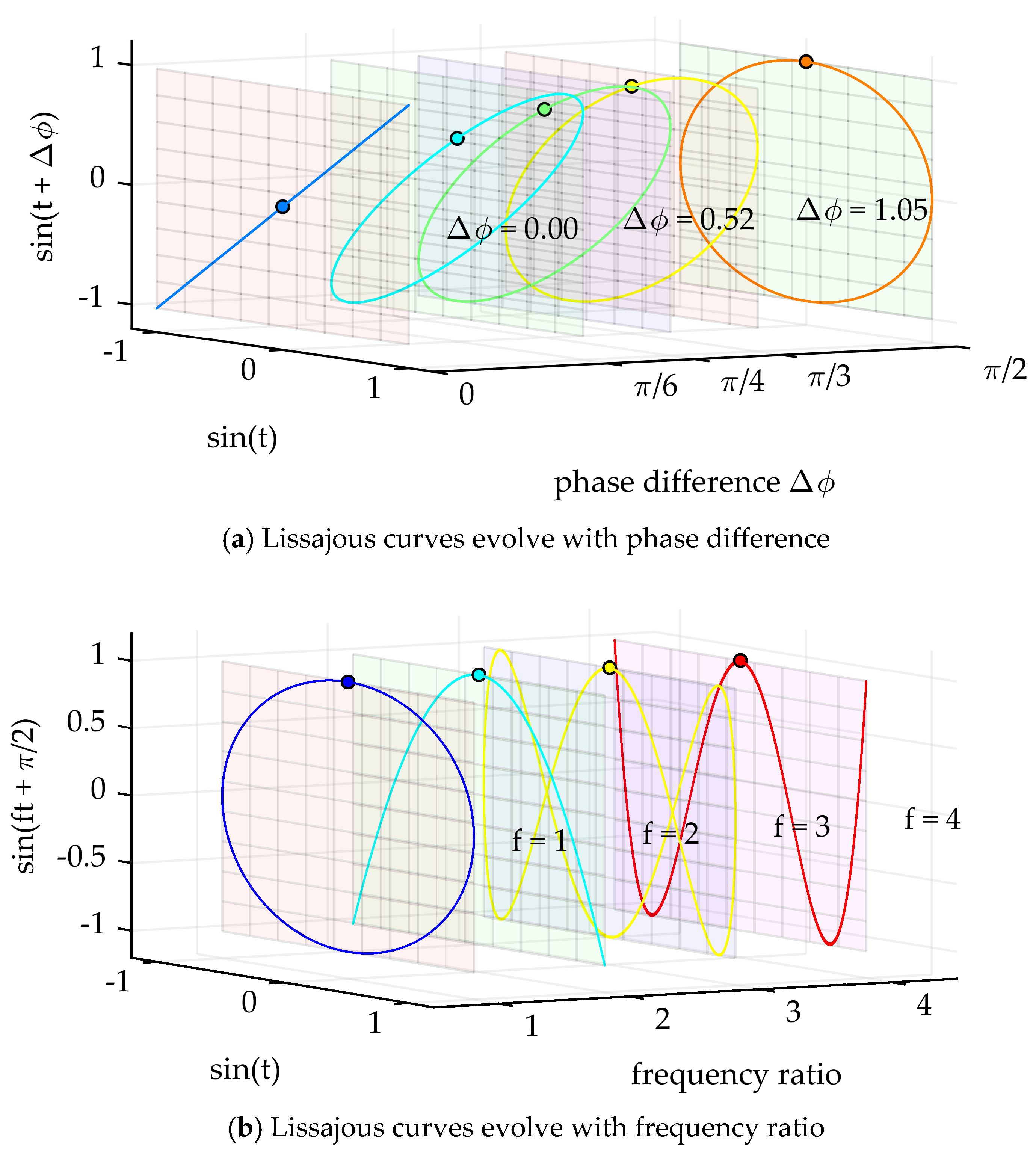
Figure 1. Schematic diagram of Lissajous curves plotted from a unit sinusoidal signal. (a) Lissajous curves with different phase differences and (b) Lissajous curves with different frequency ratios. The image uses auxiliary planes of different colors to distinguish Lissajous curves.
Energies 18 05916 g001
Figure 2. Lissajous Trajectories plotted from common signals. (a) Unit sine signal: unit circle; (b) Unit impulse function: an isosceles triangle; (c) Unit step function: U-shaped curve; (d) Unit signal function: Widen U-shaped curve.
Energies 18 05916 g002
Figure 3. Arc experiment wiring diagram: (a) schematic diagram of experimental wiring and (b) actual wiring of the experiment.
Energies 18 05916 g003
Figure 4. Measured currents for two types of loads: (a) linear loads, nearly sinusoidal, and (b) nonlinear sinusoidal distortion accompanied by a large number of random pulses.
Energies 18 05916 g004
Figure 5. Schematic diagram of the preamp circuit for nonlinear loads. Ellipsis represents other nonlinear loads.
Energies 18 05916 g005
Figure 6. Measurements to obtain normal GLT images for different load types: (a,b) linear loads with ellipsoid-like features and (c,d) nonlinear loads with a large number of distortions and closed envelope features.
Energies 18 05916 g006
Figure 7. Comparison of GLT images at SAF: (a) for linear loading, SAF induces zero rest, making the elliptical perimeter protrude, and (b) for nonlinear loading, SAF makes the perimeter appear as though it should not be closed.
Energies 18 05916 g007
Figure 8. Numerical current modeling for different load types: (a) for linear loads, where the phenomenon of zero rest and zero-rest pulses is simulated, and (b) for nonlinear loads, where the phenomenon of random pulses is simulated.
Energies 18 05916 g008
Figure 9. Validating the accuracy and generalizability of current models using the PSO algorithm.
Energies 18 05916 g009
Figure 10. Model optimization effect for one hundred random periodic cycles: (a) the sum of square error between the model and the measured current, and (b) the model-measured current correlation.
Energies 18 05916 g010
Figure 11. Schematic diagram of low-voltage user measurement circuit. The red arrow indicates the potential fault location.
Energies 18 05916 g011
Figure 12. Characteristic distributions and decision boundaries for different types of loads.
Energies 18 05916 g012
Figure 13. Scheme diagram of proposed SAF-GLT image-based detection algorithm.
Energies 18 05916 g013
Figure 14. ResNet50 model training results for linear loaded dataset.
Energies 18 05916 g014
Figure 15. ResNet50 model training results for nonlinear loaded dataset.
Energies 18 05916 g015
Figure 16. ResNet50 model training results for mixed loaded dataset.
Energies 18 05916 g016
Figure 17. Variation in the accuracy of the algorithm at different sampling rates.
Energies 18 05916 g017
Figure 18. Variation in the accuracy of the algorithm at different image sizes.
Energies 18 05916 g018
Figure 19. Schematic diagram of a comparative experiment based on the same set of raw data.
Energies 18 05916 g019
Figure 20. Comparison of results of four trajectory generation methods.
Energies 18 05916 g020
Table 1. H-transform pairs of common signals.
Original SignalImaginary PartAnalysis Signal
sin ( ω t ) sin ( ω t π 2 ) , ω > 0 sin ( ω t + π 2 ) , ω < 0 sin ( ω t ) + j sin ( ω t π 2 ) , ω > 0 sin ( ω t ) + j sin ( ω t + π 2 ) , ω < 0
δ ( t ) 1 π t δ ( t ) + j 1 π t
u ( t ) ln t π u ( t ) + j ln t π
sgn ( t ) 2 π ln t sgn ( t ) j 2 π ln t
Table 2. Parameterization of the simulation dataset.
Fault ConditionConfiguration 1SNR (dB)Sample Size
SAFlinear load t 0 , t t h e r m a l , α , C , N j , θ 25,
35,
50
30,000 each
nonlinear load α , M , C , N j , θ
mixed load t 0 , t t h e r m a l , α , M , C , N j , θ
trouble-freelinear load α , M , θ
nonlinear load
mixed load
1 The sample set is generated by traversing all parameter values, all possible load combinations, and all environmental noise conditions.
Table 3. Feature selected for modal recognition.
Feature TypeFormulaPhysical Meaning
Frequency
Domain
Odd Harmonic Distortion Ratio T H D odd = I 3 2 + I 5 2 + + I n 2 / I 1 Odd harmonics dominate in nonlinear loads
Fundamental Ratio F r = I 1 2 / I 2 Load energy concentration
Time DomainKurtosis K = E [ ( I μ ) 4 ] / δ 4 3 Current pulse sharpness
TrajectoryEllipticity E p = a / b Degree to which the trajectory is nearly elliptical
Table 4. Training results of ResNet50 on different datasets.
Different Sample SetsAcctrainAccvalPrevalRecallvalF1val
Specific conditions for trainingLinear Load99.83%99.81%99.95%99.88%99.92%
Nonlinear Load98.13%98.93%98.72%99.15%98.94%
Mixed Load97.11%97.33%98.43%96.22%97.31%
Mixed data 192%93%93%94%94%
1 Mixed datasets are the result of mixing different types of datasets for direct classification, which is significantly less effective than training on specific samples.
Table 5. Algorithm identification results (linear load).
Linear Load 1Predicted NormalPredicted Abnormal
True Normal5919 (98.65%)81 (0.68%)
True Abnormal127(1.06%)5873 (97.88%)
1 The algorithm for linear load accurately recognizes 11,792 test samples with an accuracy of 98.27% and an average elapsed time of 0.0016 s.
Table 6. Algorithm identification results (nonlinear load).
Nonlinear Load 1Predicted NormalPredicted Abnormal
True Normal5952 (99.20%)48 (0.40%)
True Abnormal236 (1.97%)5764 (96.07%)
1 The algorithm for nonlinear load accurately recognizes 11,716 test samples with an accuracy of 97.63% and an average elapsed time of 0.0016 s.
Table 7. Algorithm identification results (mixed load).
Mixed Load 1Predicted NormalPredicted Abnormal
True Normal5866 (97.77%)134 (1.12%)
True Abnormal1376 (11.47%)4624 (77.07%)
1 The algorithm for mixed load accurately recognizes 10,490 test samples with an accuracy of 87.42% and an average elapsed time of 0.0016 s.
Table 8. Comparison of algorithm identification results (nonlinear load).
MethodsAcctrAccvalNote
GLT98.13%98.93%Simple pre-processing with accurate results
MTF91.3%90.7%Complex calculations and loss of phase information
GADF92.51%90.93%Complex calculations and high sampling rate requirements
Original Waveforms93.80%89.29%Performance depends on terminal configuration
Disclaimer/Publisher’s Note: The statements, opinions and data contained in all publications are solely those of the individual author(s) and contributor(s) and not of MDPI and/or the editor(s). MDPI and/or the editor(s) disclaim responsibility for any injury to people or property resulting from any ideas, methods, instructions or products referred to in the content.