An Efficient Heuristic Algorithm for Stochastic Multi-Timescale Network Reconfiguration for Medium- and High-Voltage Distribution Networks with High Renewables

Abstract

To handle the uncertainties brought by the increasing penetration of renewable energy sources and random loads, we design a stochastic multi-timescale distribution network reconfiguration (SMTDNR) framework to coordinate diverse scheduling resources across different timescales and develop an efficient heuristic algorithm to solve this complex NP-hard combinatorial optimization problem with high efficiency for medium- and high-voltage distribution networks. First, the SMTDNR problem, incorporating distributed renewable generators, fuel generators, energy storage systems, and controllable loads, is simplified through circular constraint linearization, Jabr relaxation, and second-order cone (SOC) relaxation techniques. Then, a one-stage multi-timescale successive branch reduction (MTSBR) algorithm is developed for distribution networks with one redundant branch, which transforms the SMTDNR problem into a stochastic multi-timescale optimal power flow (SMTOPF) problem. This is extended to a two-stage MTSBR algorithm for general networks with multiple redundant branches, which iteratively runs the proposed one-stage MTSBR algorithm. Numerical results on modified IEEE 33-bus and 123-bus distribution networks validate the superior optimality, feasibility, and computational efficiency of the proposed algorithms, particularly in scenarios of high renewable penetration and increased uncertainty, offering robust and feasible solutions where traditional methods may fail.

1. Introduction

Distribution network reconfiguration (DNR) is a critical operational strategy utilized to enhance system performance (e.g., reducing power losses, alleviating line overloads and bus voltage violations, and improving overall transmission capacity) by strategically altering the status of existing sectionalizing and tie switches without the need for additional infrastructure investments [1,2,3]. Tie switches primarily interconnect the ends of adjacent radial feeders or establish connections to alternative supply points, whereas sectionalizing switches segment the main branches or sections of a single radial feeder [4]. However, DNR poses significant computational challenges due to its formulation as a complex NP-hard combinatorial optimization problem. This intractability stems from the coupling of nonconvex power flow equations with discrete (binary) switching actions, all constrained by the stringent requirement of maintaining a radial network topology. Furthermore, the pervasive uncertainty inherent in integrating high levels of renewable energy sources escalates the complexity of the DNR problem, particularly as operational decisions must span multiple interdependent timescales, and different timescale control devices must be coordinated.

To manage these uncertainties, various uncertainty optimization frameworks have been proposed, primarily encompassing stochastic, robust, and distributionally robust optimization techniques. Robust DNR approaches aim to minimize operational costs in the worst-case scenarios involving uncertain renewable outputs and loads [1]. However, this methodology can be overly conservative, potentially leading to economic inefficiency [5]. To alleviate this conservatism and prevent unnecessary losses, stochastic DNR (SDNR) incorporates statistical properties of uncertain variables and seeks to minimize the expected costs across all possible scenarios [6]. In contrast, distributionally robust DNR endeavors to minimize operational costs for the most adverse probability distributions of uncertain quantities, thereby balancing the conservativeness of robust DNR and the robustness of SDNR [2]. Despite its advantages, distributionally robust DNR incurs significantly higher computational complexity compared with SDNR, motivating our focus on the SDNR framework.

Existing methods for solving SDNR can be broadly classified into three categories: mathematical programming, heuristics/metaheuristics, and machine learning approaches. Mathematical programming methods typically transform SDNR into mixed-integer linear programs via linearization or into mixed-integer convex programs through convex relaxation techniques, such as quadratic, quadratically constrained, or conic relaxations [7]. Despite their rigor, they face scalability issues in large-scale systems, and their approximations often compromise solution accuracy and optimality guarantees. Heuristic methods exploit the topological features of distribution networks to reduce computational complexity, employing strategies such as switch opening and exchanging [8], and sequential switch opening or successive branch reduction [6,9,10]. Metaheuristic algorithms are inspired by biological or physical processes, including approaches such as hybrid particle swarm optimization [11], shuffled frog leaping [12], and hybrid simulated annealing with minimum-spanning tree algorithms [13]. Although these methods are computationally efficient, they have the disadvantages of high computational cost for evaluation, parameter dependency and tuning, and sensitivity to problem formulation and randomness. Machine learning techniques (e.g., double deep Q-learning [14] and deep reinforcement learning [15]) bypass explicit physical modeling by extracting optimal operational knowledge from historical data. However, offline training risks sub-optimal generalization, while online deployment raises safety concerns.

A notable limitation across these approaches is the limited consideration of varying timescales among different devices. Due to concerns about switch longevity and practical constraints, frequently altering switch statuses to accommodate rapid fluctuations from renewable energy sources is impractical. Conversely, distributed generators and energy storage devices can respond swiftly to maintain system power balance. To coordinate diverse scheduling resources across different timescales, a multi-timescale co-optimization framework is proposed in [16]. This framework schedules on-load tap changers on an hourly basis, dispatches the fast-acting battery energy storage system and photovoltaic inverters every 20 min, and executes DNR daily. However, this approach relies on solving the multi-timescale MISOCP problem using GAMS/Cplex, which can be computationally intensive for large-scale systems. Another study in [17] develops a bi-level Rainbow-safeDDPG algorithm, where the upper-layer Rainbow algorithm determines network topology and switching gears for on-load tap changers and switched capacitors on a slow timescale. Concurrently, the lower-layer continuous safeDDPG algorithm schedules distributed photovoltaic inverters on a fast timescale. Nonetheless, the feasibility of solutions cannot be assured due to the inherent security issues associated with deep reinforcement learning. Furthermore, both multi-timescale methods overlook the uncertainties in renewables and loads, as well as time-coupling devices such as energy storage systems.

To address these challenges, we extend our previous work on the SDNR problem by introducing a stochastic multi-timescale DNR (SMTDNR) framework and developing an efficient heuristic algorithm for medium- and high-voltage distribution networks. Model predictive control (MPC) is strategically applied to handle the uncertainties associated with loads and renewables more effectively. While prior work [18] introduced a stochastic MPC approach for dynamic and adaptive distribution network reconfiguration, it primarily addresses hourly switch operations, neglecting the coordinated control of multi-timescale devices and time-coupling devices such as the energy storage system and the ramping rate constraint of fuel generators. The primary contributions of this work are as follows:

• We design a stochastic multi-timescale rolling optimization framework that coordinates the control of various devices operating on different timescales. This framework integrates stochastic optimization with the MPC approach to effectively address uncertainties in renewables and loads and considers energy reserves to tackle these uncertainties better.
• We develop a novel heuristic algorithm to solve the SMTDNR problem with high efficiency while ensuring solution feasibility. Initially, we introduce a one-stage multi-timescale successive branch reduction (MTSBR) algorithm tailored for distribution networks with a single redundant branch. This is subsequently extended to a two-stage MTSBR algorithm applicable to general networks with multiple redundant branches through iterative application of the one-stage MTSBR method.
• We validate the optimality, feasibility, and computational efficiency of the proposed MTSBR algorithm on IEEE 33-bus and 123-bus distribution networks, considering different penetration levels of renewable generation and numbers of uncertainty scenarios.

The development of the presented algorithms stems from an extension of the SBR methodologies initially proposed in [6,19]. The SBR algorithm introduced in [19] was designed to address a deterministic DNR problem in systems without considering renewable energy sources. This was subsequently enhanced in [6] to handle a stochastic DNR problem in distribution networks characterized by high renewable energy penetration. This study further advances the framework, extending it into one-stage and two-stage MTSBR algorithms. This novel structure enables the coordinated control of energy devices operating over multiple distinct timescales within the distribution network, which is more practical for real-world applications.

The remainder of this paper is organized as follows: Section 2 presents the SMTDNR model and problem formulation. Section 3 details the one-stage and two-stage MTSBR algorithms. Section 4 provides numerical case studies, and Section 5 concludes the paper.

2. Model and Problem Formulation

2.1. Stochastic Multi-Timescale Distribution Network Reconfiguration Based on Model Predictive Control

The SMTDNR problem seeks to optimally coordinate slow-acting DNR operations with fast-acting energy resources (e.g., distributed generators and battery energy storage systems) to minimize the expected operational cost across various uncertain generation and load scenarios over a specified planning horizon. To effectively manage these uncertainties, a model predictive control framework is integrated, enabling the system to anticipate variations in renewable energy generation and loads, thereby facilitating the determination of optimal control actions for all controllable devices.

Consider a total operational period denoted by ${\mathcal{T}}_{all}$, which is examined through a sliding time window $\mathcal{T}$, which refers to the finite and fixed-length prediction horizon (i.e., the time steps) over which the optimal control actions are determined by MPC at each reconfiguration interval. For each time step $t\in {\mathcal{T}}_{all}$, the following definitions apply:

$$\begin{array}{cc}\hfill & \tau :=mod(t-1,|\mathcal{T}\left|\right),\hfill \\ \hfill & {\mathcal{T}}_1:=\{t,t+1,\dots ,t+|\mathcal{T}|-\tau -1\},\hfill \\ \hfill & {\mathcal{T}}_2:=\{t+|\mathcal{T}|-\tau ,t+|\mathcal{T}|-\tau +1,\dots ,t+|\mathcal{T}|-1\},\hfill \end{array}$$

(1)

where $\left|\mathcal{T}\right|$ denotes the number of time intervals within the window $\mathcal{T}$. As depicted in Figure 1, control actions for fast-acting devices are optimized at every time step, whereas the distribution network topology (i.e., slow-acting device branch switches) is reconfigured every $\left|\mathcal{T}\right|$ intervals. Consequently, the network topology remains fixed and radial during ${\mathcal{T}}_1$ and is subsequently re-optimized for ${\mathcal{T}}_2$, balancing operational flexibility with practical constraints on switch operations. The mathematical formulation of the SMTDNR problem for each sliding time window is detailed below.

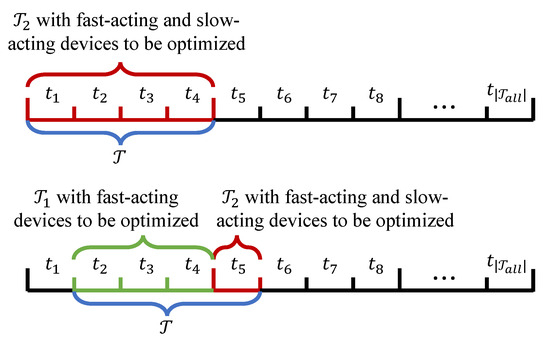
Figure 1. Illustration of the SMTDNR framework.

Consider a distribution network comprising a set of buses $i\in \mathcal{N}$ and a set of branches $ij\in \mathcal{E}$. To define the system model, we consider a distribution network characterized by a collection of nodes $\mathcal{N}$ and the paths that link them, which form the set of connections $\mathcal{E}$. For any specific connection $ij\in \mathcal{E}$ or $(i,j))\in \mathcal{E}$, we assign a consistent flow direction (for instance, always from node i to node j). The sets of substation, fuel generator, energy storage, controllable load, and non-controllable load buses are denoted by ${\mathcal{N}}_s$, ${\mathcal{N}}_G$, ${\mathcal{N}}_E$, ${\mathcal{N}}_C$, and ${\mathcal{N}}_{NC}$, respectively. The substation buses interface with the external utility or bulk power system, while the non-substation buses are interfaced with local demands and various distributed energy assets.

All branches $ij\in \mathcal{E}$ are considered switchable, encompassing both tie-line and sectionalizing switches without loss of generality. The operational condition of a switch on branch $ij$ at any time $t\in \mathcal{T}$ is captured by the Boolean decision variable ${\alpha }_{ij}^t$. The switch is considered open if ${\alpha }_{ij}^t=0$ and closed if ${\alpha }_{ij}^t=1$. The underlying uncertainty in the system, primarily arising from fluctuating renewable power output and unpredictable customer loads, is quantified by the joint probability distribution $\pi =({\pi }_w,\forall w\in \mathcal{W})$, defined across a finite collection of stochastic scenarios $\mathcal{W}$. Based on these defined components, the SMTDNR problem is constructed for optimization across each consecutive sliding time window in the operation horizon.

2.2. Objective

The objective is to minimize the expected total operational cost over all possible scenarios $\mathcal{W}$ and within the sliding time window $\mathcal{T}$. This cost encompasses fuel generator expenses, penalties for load curtailment, costs associated with energy purchases from the main grid, and benefits from energy reserves provided by fuel generators and controllable loads, as defined below:

$$\begin{array}{cc}\hfill & \mathrm{\Gamma }(\mathbf{\alpha },\mathbf{x})=\sum _{t\in \mathcal{T}}\sum _{w\in \mathcal{W}}{\pi }_w[\sum _{i\in {\mathcal{N}}_G}{C}_i\left(p_{g,i}^{w,t}\right)+C_i(p_{c,i}^{w,t},q_{c,i}^{w,t})+\hfill \\ \hfill & {\lambda }_0{p}_0^{w,t}-\sum _{i\in {\mathcal{N}}_G}({\lambda }_g^u{u}_{g,i}^{w,t}+{\lambda }_g^d{d}_{g,i}^{w,t})-\sum _{i\in {\mathcal{N}}_c}({\lambda }_c^u{u}_{c,i}^{w,t}+{\lambda }_c^d{d}_{c,i}^{w,t})],\hfill \end{array}$$

(2)

where $p_0^{w,t}$ is the power purchased from the main grid; $p_{g,i}^{w,t}$ denotes active power generation; $(p_{c,i}^{w,t},q_{c,i}^{w,t})$ represent active and reactive controllable loads; $u_{g,i}^{w,t}$ and $d_{g,i}^{w,t}$ are upward and downward reserves of the fuel generator; $u_{c,i}^{w,t}$ and $d_{c,i}^{w,t}$ denote upward and downward reserves of the controllable load; ${\lambda }_0$, ${\lambda }_g^u$, ${\lambda }_g^d$, ${\lambda }_d^u$, and ${\lambda }_d^d$ are energy pricing parameters; and $\mathbf{\alpha }$ and $\mathbf{x}$ represent decision variables for slow-acting and fast-acting devices, respectively.

The generation cost for distributed generators, denoted by $C_i\left(p_{g,i}^{w,t}\right)$, is modeled as a quadratic function:

$$C_i\left(p_{g,i}^{w,t}\right)={\rho }_a{\left(p_{g,i}^{w,t}\right)}^2+{\rho }_b{p}_{g,i}^{w,t}+{\rho }_c,$$

(3)

where ${\rho }_a$, ${\rho }_b$, and ${\rho }_c$ are predefined cost coefficients.

The cost associated with load curtailment, $C_i(p_{c,i}^{w,t},q_{c,i}^{w,t})$, is defined as

$$C_i(p_{c,i}^{w,t},q_{c,i}^{w,t})={\lambda }_c^p\left(\right|p_{c,i}^{w,t}-{\widehat{p}}_{c,i}^{w,t}|+|p_{c,i}^{w,t}-{\widehat{p}}_{c,i}^{w,t}\left|\right),$$

(4)

where ${\lambda }_c^p$ is the unit cost of load curtailment.

The third and fourth terms in the objective function account for the benefits derived from energy reserves provided by fuel generators and controllable loads, respectively.

2.2.1. Network Constraints

The following constraints apply to all buses $i,j\in \mathcal{N}$ and all branches $ij\in \mathcal{E}$, for every scenario $w\in \mathcal{W}$ at all time instances $t\in \mathcal{T}$:

$$\begin{array}{cc}\hfill & p_{ij}^{w,t}={\alpha }_{ij}^t\left[g_{ij}{\left(V_i^{w,t}\right)}^2-V_i^{w,t}{V}_j^{w,t}(b_{ij}\sin {\theta }_{ij}^{w,t}+g_{ij}\cos {\theta }_{ij}^{w,t})\right], \hfill \end{array}$$

(5)

$$\begin{array}{cc}\hfill & q_{ij}^{w,t}={\alpha }_{ij}^t\left[-b_{ij}{\left(V_i^{w,t}\right)}^2-V_i^{w,t}{V}_j^{w,t}(g_{ij}\sin {\theta }_{ij}^{w,t}-b_{ij}^{w,t}\cos {\theta }_{ij}^{w,t})\right],\hfill \end{array}$$

(6)

$$\begin{array}{cc}\hfill & {\sum }_{(i,j)\in \mathcal{E}}{p}_{ij}^{w,t}=p_i^{w,t}, \hfill \end{array}$$

(7)

$$\begin{array}{cc}\hfill & {\sum }_{(i,j)\in \mathcal{E}}{q}_{ij}^{w,t}=q_i^{w,t}, \hfill \end{array}$$

(8)

where $V_i^{w,t}$ and ${\theta }_i^{w,t}$ are the voltage magnitude and angle at bus i, respectively; ${\theta }_{ij}^{w,t}:={\theta }_i^{w,t}-{\theta }_i^{w,t}$ is the voltage angle difference across branch $(i,j)$; $(p_i^{w,t},q_i^{w,t})$ represent the active and reactive net power injections at bus i; $(p_{ij}^{w,t},q_{ij}^{w,t})$ denote the active and reactive branch power flows on branch $(i,j)$; and $g_{ij}$ and $b_{ij}$ are the series conductance and susceptance of branch $(i,j)$. Equations (5) and (6) define the active and reactive power flows on branch $(i,j)$, while Equations (7) and (8) ensure active and reactive power balance at bus i.

2.2.2. Fuel Generator Constraints

For each fuel generator located at bus $i\in {\mathcal{N}}_G$, across all scenarios $w\in \mathcal{W}$ and time instances $t\in \mathcal{T}$, the following constraints are enforced:

$$\begin{array}{cc}\hfill & p_{g,i}^{w,t}+u_{g,i}^{w,t}\le {\overline{p}}_{g,i}, \hfill \end{array}$$

(9)

$$\begin{array}{cc}\hfill & p_{g,i}^{w,t}-d_{g,i}^{w,t}\ge {\underline{p}}_{g,i}, \hfill \end{array}$$

(10)

$$\begin{array}{cc}\hfill & u_{g,i}^{w,t},d_{g,i}^{w,t},\ge 0 \hfill \end{array}$$

(11)

$$\begin{array}{cc}\hfill & {\underline{q}}_{g,i}\le q_{g,i}^{w,t}\le {\overline{q}}_{g,i}, \hfill \end{array}$$

(12)

$$\begin{array}{cc}\hfill & R{d}_{g,i}\le p_{g,i}^{w,t}-p_{g,i}^{w,t-1}\le R{u}_{g,i},\hfill \end{array}$$

(13)

where $({\overline{p}}_{g,i},{\underline{p}}_{g,i})$ and $({\overline{q}}_{g,i},{\underline{q}}_{g,i})$ represent the upper and lower bounds of active and reactive power generation of the fuel generator at bus i and $(R{d}_{g,i},R{u}_{g,i})$ denote the maximal downward and upward ramp rates of the fuel generator. Constraint (9)–(11) limit the capacity of the fuel generator. Constraint (12) restricts its reactive power output, while constraint (13) restricts the ramp rates of the fuel generator.

2.2.3. Energy Storage Constraints

For each energy storage unit at bus $i\in {\mathcal{N}}_E$, in all scenarios $w\in \mathcal{W}$ and time instances $t\in \mathcal{T}$, the following constraints apply:

$$\begin{array}{cc}\hfill & E_i^{w,t}={\kappa }_i{E}_i^{w,t-1}-p_{e,i}^{w,t}\Delta t,\hfill \end{array}$$

(14)

$$\begin{array}{cc}\hfill & {\underline{p}}_{e,i}\le p_{e,i}^{w,t}\le {\overline{p}}_{e,i}, \hfill \end{array}$$

(15)

$$\begin{array}{cc}\hfill & {\underline{E}}_i\le E_i^{w,t}\le {\overline{E}}_i, \hfill \end{array}$$

(16)

where $p_{e,i}^{w,t}$ and $E_i^{w,t}$ represent the active power output and state of charge of the energy storage at bus i, respectively; ${\kappa }_i\in (0,1)$ is the leakage rate accounting for energy loss over time; and ${\overline{E}}_i$ and ${\underline{E}}_i$ are the upper and lower limits of the energy storage capacity. Equation (14) establishes the relationship between the state of charge and the total active power output of the energy storage. Constraint (15) and (16) set the limits on the active power output and state of charge, respectively.

2.2.4. Controllable Load Constraints

For each aggregate controllable load at bus $i\in {\mathcal{N}}_C$, across all scenarios $w\in \mathcal{W}$ and time instances $t\in \mathcal{T}$, the following constraints are enforced:

$$\begin{array}{cc}\hfill & p_{c,i}^{w,t}+u_{c,i}^{w,t}\le {\widehat{p}}_{c,i}^{w,t},\hfill \end{array}$$

(17)

$$\begin{array}{cc}\hfill & p_{c,i}^{w,t}-d_{c,i}^{w,t}\ge {\underline{p}}_{c,i}^{w,t},\hfill \end{array}$$

(18)

$$\begin{array}{cc}\hfill & u_{c,i}^{w,t},u_{c,i}^{w,t}\ge 0, \hfill \end{array}$$

(19)

$$\begin{array}{cc}\hfill & {\underline{q}}_{c,i}^{w,t}\le q_{c,i}^{w,t}\le {\widehat{q}}_{c,i}^{w,t},\hfill \end{array}$$

(20)

where $(p_{c,i}^{w,t},q_{c,i}^{w,t})$ are the active and reactive power outputs for the controllable load; $(u_{c,i}^{w,t},d_{c,i}^{w,t})$ denote the upward and downward energy reserves for the controllable load; $({\widehat{p}}_{c,i}^{w,t},{\widehat{q}}_{c,i}^{w,t})$ are the forecasted active and reactive power demands; and ${\underline{p}}_{c,i}^{w,t}$ is the minimum active power demand. Constraint (17)–(19) limit the capacity of the controllable load, while constraint (20) sets the bounds for its reactive power demand.

2.2.5. Net Power Injection Constraints

For each bus $i\in \mathcal{N}$, in all scenarios $w\in \mathcal{W}$ and time instances $t\in \mathcal{T}$, the net active and reactive power injections are defined as

$$\begin{array}{cc}\hfill & p_i^{w,t}=p_{g,i}^{w,t}+p_{e,i}^{w,t}+{\widehat{p}}_{ri}^{w,t}-p_{c,i}^{w,t}-{\widehat{p}}_{nc,i}^{w,t},\hfill \end{array}$$

(21)

$$\begin{array}{cc}\hfill & q_i^{w,t}=q_{g,i}^{w,t}+{\widehat{q}}_{ri}^{w,t}-q_{c,i}^{w,t}-{\widehat{q}}_{nc,i}^{w,t}, \hfill \end{array}$$

(22)

where $(p_{nc,i}^{w,t}$ and $q_{nc,i}^{w,t})$ denote the active and reactive power consumption of the aggregate non-controllable load, respectively, and ${\widehat{p}}_{ri}^{w,t}$ and ${\widehat{q}}_{ri}^{w,t}$ are the active and reactive power outputs of the aggregate renewable energy source, respectively. Both $({\widehat{p}}_{nc,i}^{w,t},{\widehat{p}}_{nc,i}^{w,t})$ and $({\widehat{p}}_{ri}^{w,t},{\widehat{q}}_{ri}^{w,t})$ are uncertain parameters with a probability distribution $\mathit{\pi }$ over scenarios $w\in \mathcal{W}$. Equations (21) and (22) restrict the active and reactive net power injections at each bus.

2.2.6. Branch Thermal Limits

For each branch $ij\in \mathcal{E}$, in all scenarios $w\in \mathcal{W}$ and time instances $t\in \mathcal{T}$, the apparent power flow must respect the thermal limit:

$${\left(p_{ij}^{w,t}\right)}^2+{\left(q_{ij}^{w,t}\right)}^2\le {\overline{s}}_{ij}^2,$$

(23)

where ${\overline{s}}_{ij}$ is the branch transmission capacity of branch $(i,j)$. To enhance computational efficiency, the nonlinear constraint in (23) can be linearized using the circular constraint linearization method [20] as follows:

$$\begin{array}{cc}\hfill & -{\overline{s}}_{ij}\le p_{ij}^{w,t}\le {\overline{s}}_{ij}, \hfill \end{array}$$

(24)

$$\begin{array}{cc}\hfill & -{\overline{s}}_{ij}\le q_{ij}^{w,t}\le {\overline{s}}_{ij}, \hfill \end{array}$$

(25)

$$\begin{array}{cc}\hfill & -\sqrt{2}{\overline{s}}_{ij}\le p_{ij}^{w,t}+q_{ij}^{w,t}\le \sqrt{2}{\overline{s}}_{ij},\hfill \end{array}$$

(26)

$$\begin{array}{cc}\hfill & -\sqrt{2}{\overline{s}}_{ij}\le p_{ij}^{w,t}-q_{ij}^{w,t}\le \sqrt{2}{\overline{s}}_{ij}.\hfill \end{array}$$

(27)

2.2.7. Voltage Limits

For each bus $i\in \mathcal{N}$ and all branches $ij\in \mathcal{E}$ across all scenarios $w\in \mathcal{W}$ and time instances $t\in \mathcal{T}$, voltage magnitudes and angles are bounded as

$$\begin{array}{c}\hfill {\underline{V}}_i\le V_i^{w,t}\le {\overline{V}}_i,\end{array}$$

(28)

$$\begin{array}{c}\hfill {\underline{\theta }}_{ij}\le {\theta }_{ij}^{w,t}\le {\overline{\theta }}_{ij},\end{array}$$

(29)

where $({\underline{V}}_i,{\overline{V}}_i)$ represent the lower and upper bounds for voltage magnitude at bus i and $({\underline{\theta }}_{i}j,{\overline{\theta }}_{i}j)$ represent the lower and upper bounds for voltage angle difference across branch $(i,j)$.

2.2.8. Network Topology Constraints

Let the network graph with switch statuses $\mathbf{\alpha }=({\alpha }_{ij}^t,\forall ij\in \mathcal{E},\forall t\in \mathcal{T})$ be denoted by $\mathcal{G}\left(\mathbf{\alpha }\right)$. The feasible set of $\mathbf{\alpha }$, denoted by $\mathcal{A}$, can be defined to ensure a radial topology [6]:

$$\begin{array}{cc}\hfill \mathcal{A}:=\{\mathbf{\alpha } |& \mathcal{G}\left(\mathbf{\alpha }\right) \mathrm{has} \mathrm{no} \mathrm{loop}; \mathrm{and} \mathrm{each} \mathrm{bus} \mathrm{in} \mathcal{N}/{\mathcal{N}}_s\hfill \\ \hfill & \mathrm{is} \mathrm{connected} \mathrm{to} \mathrm{a} \mathrm{single} \mathrm{bus} \mathrm{in} {\mathcal{N}}_s\}.\hfill \end{array}$$

A network graph $\mathcal{G}\left(\mathbf{\alpha }\right)$ is radial if and only if $\mathbf{\alpha }|\in \mathcal{A}$.

2.3. SMTDNR Problem Formulation

Combining the objective and all constraints, the SMTDNR problem for each sliding time window $\mathcal{T}$ is formulated as a mixed-integer nonlinear and nonconvex optimization problem:

$$\begin{array}{cc}\hfill \mathbf{SMTDNR}& : \min \mathrm{\Gamma }(\mathit{\alpha },\mathit{x})\hfill \\ \hfill \mathrm{over} \mathit{\alpha }& :=({\alpha }_{ij}^t, \forall ij\in \mathcal{E}, \forall t\in {\mathcal{T}}_2)\in \mathcal{A},\hfill \\ \hfill \mathit{x}& :=({\mathbf{x}}^{w,t}, \forall w\in \mathcal{W}, \forall t\in \mathcal{T})\hfill \\ \hfill & :=\left(p_{g,i}^{w,t},q_{g,i}^{w,t},\forall i\in {\mathcal{N}}_G;p_{e,i}^{w,t},\forall i\in {\mathcal{N}}_E;p_{c,i}^{w,t},q_{c,i}^{w,t},\right.\hfill \\ \hfill & \left.\forall i\in {\mathcal{N}}_C;V_i^{w,t},{\theta }_i^{w,t},\forall i\in \mathcal{N};\forall w\in \mathcal{W},\forall t\in \mathcal{T}\right).\hfill \\ \hfill \mathrm{s.t.}& \left(5\right)–\left(22\right), \left(24\right)–\left(29\right).\hfill \end{array}$$

To efficiently solve this intricate problem, relaxation techniques and a simplified power flow model are introduced in subsequent subsections.

2.4. Jabr Relaxation

To expedite computation, Jabr relaxation is employed to obtain a second-order cone (SOC) relaxation of the SMTDNR problem. For every bus $i\in \mathcal{N}$, an auxiliary variable $v_i^{w,t}={\left|V_i^{w,t}\right|}^2$ is introduced. For every branch $(i,j)\in \mathcal{E}$, auxiliary variables $c_{ij}^{w,t}=|V_i^{w,t}\left|\right|V_j^{w,t}|\cos \left({\theta }_{ij}^{w,t}\right)$ and $s_{ij}^{w,t}=|V_i^{w,t}\left|\right|V_j^{w,t}|\sin \left({\theta }_{ij}^{w,t}\right)$ are defined. With these auxiliary variables, the branch flow equations in (5) and (6) can be reformulated as follows for $\forall i,j\in \mathcal{N}$, $\forall ij\in \mathcal{E}$, $\forall w\in \mathcal{W}$, and $\forall t\in \mathcal{T}$:

$$\begin{array}{cc}\hfill & p_{ij}^{w,t}={\alpha }_{ij}^t(g_{ij}{v}_i^{w,t}-g_{ij}{c}_{ij}^{w,t}-b_{ij}{s}_{ij}^{w,t}),\hfill \end{array}$$

(30)

$$\begin{array}{cc}\hfill & q_{ij}^{w,t}={\alpha }_{ij}^t(-b_{ij}{v}_i^{w,t}+b_{ij}{c}_{ij}^{w,t}-g_{ij}{s}_{ij}^{w,t}).\hfill \end{array}$$

(31)

The nonconvex definitions of variables $v_i^{w,t}$, $c_{ij}^{w,t}$, and $s_{ij}^{w,t}$ are relaxed by adding the following rotated cone constraints:

$${\left(c_{ij}^{w,t}\right)}^2+{\left(s_{ij}^{w,t}\right)}^2\le v_i^{w,t}{v}_j^{w,t},\forall ij\in \mathcal{E},\forall w\in \mathcal{W},\forall t\in \mathcal{T}.$$

(32)

Thus, the SMTDNR problem with Jabr relaxation, denoted by SMTDNR-J, is formulated as

$$\begin{array}{cc}\hfill \mathbf{SMTDNR-J}: & \min \mathrm{\Gamma }(\mathit{\alpha },\mathit{x})\hfill \\ \hfill \mathrm{s.t.} & \left(7\right)–\left(27\right), \left(30\right)–\left(32\right),\hfill \\ \hfill & \forall w\in \mathcal{W},\forall t\in \mathcal{T}.\hfill \end{array}$$

2.5. DistFlow Model for Radial Topology

For a radial power network with fixed switch statuses $\mathit{\alpha }$, the network constraints in (5) and (6) can be equivalently represented using the DistFlow model. For all $i,j\in \mathcal{N}$, $ij\in \mathcal{E}$, $w\in \mathcal{W}$, and $t\in \mathcal{T}$,

$$\begin{array}{c}\sum _{ij\in \mathcal{E}}\left(p_{ij}^{w,t}-r_{ij}{l}_{ij}^{w,t}\right)+p_j^{w,t}=\sum _{jk\in \mathcal{E}}{p}_{jk}^{w,t}, \hfill \end{array}$$

(33)

$$\begin{array}{c}\sum _{ij\in \mathcal{E}}\left(q_{ij}^{w,t}-x_{ij}{l}_{ij}^{w,t}\right)+q_j^{w,t}=\sum _{jk\in \mathcal{E}}{q}_{jk}^{w,t}, \hfill \end{array}$$

(34)

$$\begin{array}{c}{v}_i^{w,t}-v_j^{w,t}\ge 2(r_{ij}{p}_{ij}^{w,t}+x_{ij}{q}_{ij}^{w,t})-(r_{ij}^2+x_{ij}^2)l_{ij}^{w,t}\hfill \\ -M(1-{\alpha }_{ij}^t),\hfill \end{array}$$

(35)

$$\begin{array}{c}{v}_i^{w,t}-v_j^{w,t}\le 2(r_{ij}{p}_{ij}^{w,t}+x_{ij}{q}_{ij}^{w,t})-(r_{ij}^2+x_{ij}^2)l_{ij}^{w,t}\hfill \\ +M(1-{\alpha }_{ij}^t),\hfill \end{array}$$

(36)

$$\begin{array}{c}{l}_{ij}^{w,t}{v}_i^{w,t}={\left(p_{ij}^{w,t}\right)}^2+{\left(q_{ij}^{w,t}\right)}^2, \hfill \end{array}$$

(37)

where $r_{ij}$ and $x_{ij}$ are the resistance and reactance of branch $(i,j)$, respectively; $l_{ij}^{w,t}$ denotes the squared current of branch $(i,j)$; and M is a sufficiently large positive constant used in the big-M formulation. Constraint (35) and (36) enforce the voltage drop across branch $(i,j)$ when ${\alpha }_{ij}^t=1$. The big-M formulation relaxes the voltage coupling between buses i and j when ${\alpha }_{ij}^t=0$ (i.e., the line is disconnected). Constraint (33) and (34) ensure active and reactive power balance at each bus, respectively. Quadratic constraint (37) introduces nonconvexity, which is convexified via the SOC relaxation below:

$$l_{ij}^{w,t}{v}_i^{w,t}\ge {\left(p_{ij}^{w,t}\right)}^2+{\left(q_{ij}^{w,t}\right)}^2.$$

(38)

Additionally, the voltage constraint in (28) is replaced by

$${\left({\underline{V}}_i\right)}^2\le v_i^{w,t}\le {\left({\overline{V}}_i\right)}^2, \forall i\in \mathcal{N},\forall w\in \mathcal{W},\forall t\in \mathcal{T}.$$

(39)

2.6. Multi-Timescale Optimal Power Flow Model

For a given and fixed network topology with switch statuses $\mathit{\alpha }$, the SMTDNR problem reduces to a stochastic multi-timescale optimal power flow (SMTOPF) problem as follows:

$$\begin{array}{ccc}& & \mathrm{SMTOPF}\left(\mathit{\alpha }\right): \min \mathrm{\Gamma }\left(\mathit{x}\right)\hfill \\ & & \mathrm{s.t.} \left(9\right)–\left(27\right), \left(30\right)–\left(32\right), \forall w\in \mathcal{W},\forall t\in \mathcal{T}.\hfill \end{array}$$

For a radial network, the SMTOPF problem can be further simplified by employing the DistFlow model, resulting in

$$\begin{array}{c}\mathbf{SMTOPF-Radial}\left(\mathit{\alpha }\right): \min \mathrm{\Gamma }\left(\mathit{x}\right)\hfill \\ \mathrm{s.t.} \left(9\right)–\left(27\right), \left(33\right)–\left(39\right), \forall w\in \mathcal{W},\forall t\in \mathcal{T}.\hfill \end{array}$$

Since only the network topology during $t\in {\mathcal{T}}_2$ needs optimization, the SMTOPF problem can be formulated as a mixed model to improve computational efficiency, referred to as SMTOPF-Mix$\left(\alpha \right)$:

$$\begin{array}{ccc}& & \mathbf{SMTOPF-Mix}\left(\mathit{\alpha }\right): \min \mathrm{\Gamma }\left(\mathit{x}\right)\hfill \\ & & \mathrm{s.t.} \left(9\right)–\left(27\right), \left(33\right)–\left(39\right), \forall w\in \mathcal{W},\forall t\in {\mathcal{T}}_1.\hfill \\ & & \left(9\right)–\left(27\right), \left(30\right)–\left(32\right), \forall w\in \mathcal{W},\forall t\in {\mathcal{T}}_2.\hfill \end{array}$$

In this mixed formulation, DistFlow model (33)–(37) is applied to the radial network topology for time intervals ${\mathcal{T}}_1$, while the more general Jabr relaxation in (30)–(32) is employed for ${\mathcal{T}}_2$, where the topology is being optimized. Notably, when $\tau =0$, the problem $\mathrm{SMTOPF}-\mathrm{Mix}\left(\mathit{\alpha }\right)$ is equivalent to $\mathrm{SMTOPF}\left(\mathit{\alpha }\right)$.

3. Multi-Timescale Successive Branch Reduction Algorithm

3.1. One-Stage Multi-Timescale Successive Branch Reduction Algorithm

The algorithms presented herein build upon the SBR methodology previously developed in [6] for the SDNR problem. The new contribution lies in their ability to coordinate optimal control across multi-timescale devices. We will, therefore, bypass common elements and theoretical justifications to concentrate on the distinguishing components of this extension. Consistently with the finding in [6] that aggregating multiple substations does not affect the efficacy of the algorithm, a singular substation bus is presumed for the distribution network throughout this formulation.

For clarification, we start with the specific network configuration with a single redundant branch and present a one-stage multi-timescale SBR (MTSBR) algorithm, Algorithm 1, which contains the following steps:

Algorithm 1: One-stage MTSBR.

3.1.1. Initialization (Line 1)

For time intervals $t\in {\mathcal{T}}_1$, the branch statuses are known and fixed, typically from a prior optimization or initial configuration. For time intervals $t\in {\mathcal{T}}_2$, all branches (including the redundant branch) are initially considered closed.

3.1.2. Divide the Loop into Sub-Paths (Lines 2–3)

Let us define the sole loop structure of the network by $\mathcal{P}$ and the set of buses in the loop by ${\mathcal{N}}_{\mathcal{P}}$. Based on the optimal solution ${\mathit{x}}_{\mathcal{E}}$ of $\mathrm{SMTOPF-Mix}\left({\mathit{\alpha }}_{\mathcal{E}}\right)$, the expected active power injection into loop $\mathcal{P}$ is defined as

$$\begin{array}{c}\hfill {\tilde{p}}_i^{\mathcal{P}}:={\displaystyle \frac{1}{|{\mathcal{T}}_2\left|\right|\mathcal{W}|}}\sum _{t\in {\mathcal{T}}_2}\sum _{w\in \mathcal{W}}\sum _{\begin{array}{c}j:i\sim j and\\ j\in {\mathcal{N}}_{\mathcal{P}}\end{array}}{p}_{ij}^{w,t},\end{array}$$

(40)

The buses with positive expected active power injection (${\tilde{p}}_i^{\mathcal{P}}>0$) are installed with or are equivalent to distributed energy sources and divide the loop into several sub-paths $\left\{{\mathcal{P}}_1,\dots ,{\mathcal{P}}_{n_r}\right\}$.

3.1.3. Identify the Candidate Branches (Lines 4–8)

Let us define the expected active power flow for branch $ij\in {\mathcal{P}}_m$ as follows:

$$\begin{array}{c}\hfill {\tilde{p}}_{ij}:={\displaystyle \frac{1}{|{\mathcal{T}}_2\left|\right|\mathcal{W}|}}\sum _{t\in {\mathcal{T}}_2}\sum _{w\in \mathcal{W}}{p}_{ij}^{w,t}.\end{array}$$

(41)

For each sub-path ${\mathcal{P}}_m$, we find the branch with the minimum expected active power flow and denote it by ${\widehat{e}}_m$. Then, we denote the upstream neighbor incident to the head node i by ${\widehat{e}}_m^{\mathrm{up}}$ and the downstream neighbor incident to the tail node j by ${\widehat{e}}_m^{\mathrm{down}}$. Both ${\widehat{e}}_m^{\mathrm{up}}$ and ${\widehat{e}}_m^{\mathrm{down}}$ are in loop ${\mathcal{P}}_m$. For each branch ${\widehat{e}}_m$, a subset of candidate branches, $\mathcal{K}\left({\widehat{e}}_m\right)$, is identified as follows:

$$\begin{array}{ccc}& \mathcal{K}\left({\widehat{e}}_m\right)& :=\left\{\begin{array}{cc}\{{\widehat{e}}_m,{\widehat{e}}_m^{\mathrm{down}}\},\hfill & \mathrm{if} {\tilde{p}}_{{\widehat{e}}_m}>0 \mathrm{and} {\widehat{e}}_m^{\mathrm{down}} \mathrm{exists};\hfill \\ \{{\widehat{e}}_m,{\widehat{e}}_m^{\mathrm{up}}\},\hfill & \mathrm{if} {\tilde{p}}_{{\widehat{e}}_m}<0 \mathrm{and} {\widehat{e}}_m^{\mathrm{up}} \mathrm{exists};\hfill \\ \left\{{\widehat{e}}_m\right\},\hfill & \mathrm{otherwise}.\hfill \end{array}\right.\hfill \end{array}$$

Finally, the union of $\mathcal{K}\left({\widehat{e}}_m\right)$ from all sub-paths forms the candidate branch set ${\mathcal{E}}_c$.

3.1.4. Identify the Optimal Branch in Each Sub-Path (Lines 9–12)

First, we open one candidate branch $e\in {\mathcal{E}}_c$ and keep the other branches close to form a radial network. Then, we solve $\mathrm{SMTOPF-Radial}\left({\mathit{\alpha }}_{\mathcal{E}}\left(e\right)\right)$ to get the objective value.

3.1.5. Get the Optimal Solution (Lines 13–14)

Among all solutions of $\mathrm{SMTOPF-Radial}\left({\mathit{\alpha }}_{\mathcal{E}}\left(e\right)\right)$, we find the one with the minimum objective value.

The adaptation of Algorithm 1 for networks that feature both controllable and fixed (uncontrollable) branches is achieved via targeted restrictions on the optimization domain. The algorithm is implemented by confining the branch search (Line 6) to controllable assets and excluding uncontrollable branches from the set of selectable candidates ${\cup }_{m=1}^{n_r}\mathcal{K}\left({\widehat{e}}_m\right)$ (Line 8), specifically within the network topology optimization phase ($t\in {\mathcal{T}}_2$). Crucially, this work refines the approach in [6] by computing the expected power injections (${\tilde{p}}_i^{\mathcal{P}}$) and flows (${\tilde{p}}_{ij}$) specifically for the $t\in {\mathcal{T}}_2$ period. For modeling simplicity, the formulation employs a mixed methodology that integrates the properties of the DistFlow approximation with the Jabr relaxation.

3.2. Two-Stage Multi-Timescale Successive Branch Reduction Algorithm

For general networks with more than one redundant branch or chordless loop, the one-stage MTSBR approach (Algorithm 1) is extended into a two-stage MTSBR approach, denoted Algorithm 2. Without loss of generalization, we assume the distribution network to have $L>1$ redundant branches, characterized by L chordless loops ${\mathcal{P}}^l$, $l=1,\dots ,L$. A detailed implementation of Algorithm 2 is presented below.

3.2.1. Initial Radial Topology Determination (Lines 1–11)

The first stage aims to obtain the initial radial network for the second stage, which contains the following steps:

Step 1:

Similar to Algorithm 1, the initial branch statuses are fixed and known for the time intervals $t\in {\mathcal{T}}_1$ and are presumed closed for the subsequent intervals $t\in {\mathcal{T}}_2$ (Line 1). Based on this initialization, the $\mathrm{SMTOPF-Mix}\left({\mathit{\alpha }}_{\mathcal{E}}\right)$ problem is solved to obtain the initial operating state (Line 3).

Step 2:

The branch in each existing network loop that exhibits the minimum expected active power flow is identified and sequentially opened (Lines 5–7). A necessary step involves updating the set of affected loops when an opened branch is common to two or more such loops (Lines 8–10). This operation continues until a radial topology is realized.

Step 3:

The collective set of branches opened during this initial stage, ${\mathcal{E}}^o$, constitutes the initial candidate set of open branches for the subsequent refinement stage (Line 12).

Algorithm 2: Two-stage MTSBR.

3.2.2. Second-Stage Iterative Refinement (Lines 12–25)

The second stage implements an iterative refinement procedure to search for the optimal radial topology, containing the following steps:

Step 1:

Each branch within the initial candidate set ${\mathcal{E}}^o$ is closed alternatively (Line 16). Each of these closures introduces a single redundancy, creating L distinct loops in the network.

Step 2:

For every resulting network configuration (i.e., corresponding to each of the L loops), Algorithm 1 is then invoked to identify an improved open branch, which subsequently updates the candidate set ${\mathcal{E}}^o$. This close-and-open refinement is executed over successive outer iterations. This operation continues until a radial topology is realized.

Step 3:

The optimal radial topology is identified throughout all inner and outer iterations for time intervals $t\in {\mathcal{T}}_2$, along with the corresponding control settings for all fast-acting devices throughout the entire time horizon $t\in \mathcal{T}$.

A significant benefit of the proposed algorithms is the guarantee of solution feasibility. This assurance is inherently secured through the requirement to solve the SMTOPF problem for every feasible candidate topology, a step explicitly mandated in Line 11 of Algorithm 1 and Line 17 of Algorithm 2. Notwithstanding the guaranteed feasibility, it is pertinent to note that global optimality of the solutions cannot be strictly ensured. A formal investigation into the existence and magnitude of any resulting optimality gaps presents a promising direction for future research.

4. Results

4.1. Experimental Setup

To validate the proposed approach, numerical experiments were conducted on modified IEEE 33-bus and 123-bus distribution networks. The modified IEEE 33-bus system, depicted in Figure 2, includes a substation with two fuel generators (Buses 3 and 30, marked by dark purple squares), two renewable energy resource buses (Buses 4 and 9, each with a small wind turbine and solar panel, marked by light purple squares), two energy storage buses (Buses 7 and 15, marked by blue squares), two aggregated controllable load buses (Buses 14 and 29, marked by green circles), and non-controllable load buses. For the modified IEEE 123-bus system (Figure 3), fuel generators are at Buses 2 and 36, renewable resources at Buses 14 and 25, energy storage at Buses 100 and 118, and aggregated controllable loads at Buses 51 and 65, with other buses being non-controllable loads. The black lines represent the initially closed branches, while the red dashed lines represent the redundant branches of the test systems in Figure 2 and Figure 3.

Figure 2. Modified IEEE 33-bus distribution network with 5 redundant branches.

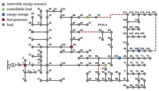
Figure 3. Modified IEEE 123-bus distribution network with 5 redundant branches.

Uncertainty scenarios were generated using hourly load, wind, and solar generation data from Germany in 2019 [21]. Note that the algorithmic efficiency and convergence of the proposed heuristic are independent of the specific input data set. Twenty-four-hour daily vectors for these parameters were concatenated into 365 daily vectors. These vectors were then scaled to match IEEE network capacities and then clustered using the classical k-medoids method. This widely adopted technique derives the probability distribution of generation and loads, and the choice of clustering method does not affect the algorithm’s applicability. The optimal number of scenarios was determined using the Silhouette criterion clustering evaluation method, with Figure 4 showing that two clusters yielded the highest silhouette value, indicating optimal clustering at two scenarios. Reactive power for renewable generation was determined using fixed power factors [8].

Figure 4. Silhouette criterion clustering evaluation result.

Key simulation parameters were configured as follows: bus voltage limits ${\underline{V}}_i=0.95$ p.u. and ${\overline{V}}_i=1.05$ p.u.; branch thermal limit ${\overline{s}}_{ij}=0.1 \mathrm{p}.\mathrm{u}.$; time horizon $\left|\mathcal{T}\right|=4 \mathrm{h}$ with total period $|{\mathcal{T}}_{all}|=24$ h; fuel generator ramp rates $R{d}_{g,i}=-0.7 {\overline{p}}_{g,i}$ and $R{u}_{g,i}=0.7 {\overline{p}}_{g,i}$; energy storage efficiency ${\eta }_{c,i}=0.9$, leakage rate ${\kappa }_i=1$, maximum power ${\overline{p}}_{e,i}=1$ p.u., minimum power ${\underline{p}}_{e,i}=-1$ p.u., maximum capacity $\overline{E}=20 \mathrm{p}.\mathrm{u}.$, and initial state of charge $E_0=2$ p.u.; and reserve prices ${\lambda }_g^u={\lambda }_g^d={\lambda }_d^u={\lambda }_d^d=1$. All experiments were conducted on a Windows 64-bit system equipped with an Intel Core i7-10875H 8-core CPU and 16 GB of RAM from LENOVO, Beijing, China. The commercial solver Gurobi was utilized to solve the optimization problems.

The proposed method was benchmarked against two alternative approaches to assess its optimality and computational efficiency:

• Method 1: Mathematical Programming with Convexified DistFlow Model. This approach replaces the exact power flow Equations (5) and (6) with the SOC relaxed DistFlow model (Section 2.5) to reduce computational complexity.
• Method 2: Mathematical Programming with Linearized DistFlow Model. This method employs the linearized DistFlow equations, as a further simplification of the power flow constraints.

Due to the highly nonconvex nature and the large-scale, combined combinatorial and continuous structure of the proposed stochastic multi-timescale rolling reconfiguration model, deriving a non-trivial and generalizable theoretical optimality gap guarantee is currently mathematically intractable. To provide a quantitative validation of the proposed algorithms, we adopt the standard practice for complex power system heuristics, i.e., rigorous empirical analysis against proven high-quality benchmarks. Method 1, using a convexified DistFlow model, served as the benchmark for defining the relative errors (optimality gap) of the other comparison methods.

4.2. Optimality of One-Stage Multi-Timescale Successive Branch Reduction Algorithm

Experiments were first performed using the one-stage MTSBR algorithm (Algorithm 1) on the modified IEEE 33-bus distribution network, where each initial redundant branch shown in Figure 2 is individually closed to create a single-redundant-branch network scenario.

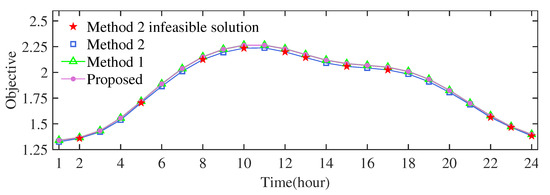
Table 1 presents the mean and maximum relative errors of the objective function for Algorithm 1 (proposed) and Method 2 in different scenarios. As observed in Table 1, Algorithm 1 consistently exhibited a negligible relative error, with a maximum observed error of only 0.261%. In contrast, for initial redundant branches (8, 21), (12, 22), (18, 33), and (2, 29), Method 2 frequently yielded solutions infeasible for the original SMTDNR problem, which incorporates nonconvex power flow Equations (6)–(8). These infeasible instances are denoted by “*” in Table 1 and marked by red stars in Figure 5. Figure 5 further illustrates the objective values over a 24 h period, specifically for the (2, 29) scenario as an example, clearly showing the infeasible solutions of Method 2. In summary, Algorithm 1 demonstrates competitive optimality compared with benchmark Method 1, which uses the SOC-relaxed DistFlow model, and significantly superior feasibility compared with Method 2, which uses the linearized DistFlow model.

Table 1. Relative errors in objective (IEEE 33-bus network with a single redundant branch).

Initial Redundant Branch	Algorithm 1 (Proposed) vs. Method 1		Method 2 vs. Method 1
	Mean (%)	Max (%)	Mean (%)	Max (%)
(8, 21)	0.013	0.261	−0.887 *	−0.072 *
(9, 15)	−0.001	0.000	−0.923	−0.392
(12, 22)	0.026	0.176	−0.893 *	−0.408 *
(18, 33)	−0.001	0.004	−0.704 *	−0.053 *
(2, 29)	−0.001	−0.001	−1.090 *	−0.475 *

*: The solution is infeasible for the original network constraints in (5)–(8).

Figure 5. Objective in the IEEE 33-bus network with initial redundant branch (2, 29). Points marked in red for Method 2 indicate solutions infeasible for the original network constraints in (5)–(8).

4.3. Optimality of Two-Stage Multi-Timescale Successive Branch Reduction Algorithm

The effectiveness of the proposed two-stage SBR algorithm (Algorithm 2) was evaluated on the IEEE 33-bus network, augmented with five redundant branches, two fuel generators, two energy storage systems, and two controllable loads (Figure 2).

4.3.1. Impact of Renewable Penetration Levels

Figure 6 illustrates the temporal evolution of the objective value over a 24 h horizon under different renewable energy resource penetration levels, where the penetration coefficient $k_r$ uniformly scales the power output of renewable energy resources. As $k_r$ increases, Method 2 (with linearization) exhibits noticeable performance degradation, frequently producing solutions that violate the original network constraints in (5)–(8). Method 1 performs the worst, often failing to converge to a feasible configuration across the majority of the time series. In contrast, the proposed method, Algorithm 2, consistently delivers feasible, high-quality solutions throughout the simulation, outperforming both benchmarks in optimality and feasibility.

Figure 6. Objective in the IEEE 33-bus network under different renewable penetration levels: (a) $k_r=1$, (b) $k_r=2$, and (c) $k_r=3$. Load level $k_l=1.0$. Number of uncertainty scenarios $\left|\mathcal{W}\right|=2$. Missing data points indicate that solver does not converge. Points marked in red stars indicate infeasible solutions for nonconvex network constraints in (5)–(8).

4.3.2. Impact of Number of Scenarios

The influence of the number of uncertainty scenarios, $\left|\mathcal{W}\right|$, on the optimization methods is illustrated in Figure 7. As $\left|\mathcal{W}\right|$ increases, both Method 1 and Method 2 increasingly struggle to achieve feasible solutions or generate solutions violating the nonconvex network constraints in (5)–(8). Conversely, the proposed method, Algorithm 2, maintains robust feasibility, with only marginal degradation in objective values as the number of scenarios increases. A consistent trend is observed across all test cases: the advantages of the proposed method, Algorithm 2, become more pronounced with more redundant branches, higher renewable penetration levels, and increased uncertainty dimensionality. This is attributed to the escalating number of binary switching decisions and nonconvex and nonlinear network constraints in (5)–(8), which substantially amplify the computational burden and sub-optimality risk for conventional mixed-integer nonlinear programming solvers. By transforming the SMTDNR problem into multiple SMTOPF problems, Algorithm 2 effectively mitigates these challenges, leading to superior solution quality and computational reliability.

Figure 7. Objective in the IEEE 33-bus network under different numbers of scenarios: (a) $\left|\mathcal{W}\right|=2$ and (b) $\left|\mathcal{W}\right|=4$. Missing data points indicate that solver does not converge. Points marked in red stars indicate infeasible solutions for nonconvex network constraints in (5)–(8).

4.4. Scalability of Two-Stage MTSBR

To further demonstrate the scalability of the proposed two-stage MTSBR algorithm (Algorithm 2), experiments were conducted on the IEEE 123-bus network, specifically augmented to include five redundant branches, two fuel generators, two energy storage systems, and two controllable loads (see Figure 3). Similar to Section 4.2, Method 1 is used as a trustworthy benchmark for relative error assessment.

Table 2 presents the relative errors in the objective function (compared with Method 1) under different renewable penetration levels, where $k_r$ proportionally scales the power output of renewable power sources. Infeasible instances are marked with an asterisk (“*”) in Table 2 and red stars in Figure 8. The results indicate that the proposed algorithm consistently exhibits minor relative errors in the objective, specifically less than 0.025%. In contrast, Method 2 exhibits significantly larger relative errors, ranging from over 1.5% to 4.5%. Crucially, all solutions from Method 2 were found to be infeasible for the original nonconvex power flow constraints in (5)–(8), whereas all solutions generated by the proposed algorithm remained feasible. These findings are further corroborated by Figure 8, which illustrates objective value distribution over a 24 h period for $k_r=3$. This comprehensive analysis underscores the superior scalability, robustness, and solution quality of the proposed two-stage MTSBR algorithm.

Table 2. Relative errors in objective under different renewable penetration levels (IEEE 123-bus network with five redundant branches).

${\mathit{k}}_{\mathit{r}}$	Method	Mean (%)	Max (%)
1	Proposed	0.007	0.025
	Method 2	1.752 *	4.500 *
2	Proposed	0.007	0.017
	Method 2	1.655 *	4.328 *
3	Proposed	0.005	0.017
	Method2	1.588 *	4.116 *

*: The solution is infeasible for network constraints in (5)–(8).

Figure 8. Objective in the IEEE 123-bus network under renewable penetration levels $k_r=3$. Load level $k_l=1.0$. Number of uncertainty scenarios $\left|\mathcal{W}\right|=2$. Points marked in red for Method 2 indicate solutions infeasible for network constraints in (5)–(8).

4.5. Computational Efficiency

The computational efficiency of the proposed two-stage MTSBR algorithm (Algorithm 2) is verified by comparing its Gurobi “solvertime” with that of Method 1 and Method 2.

Table 3 presents the mean computation time of all three methods over a 24 h period under different renewable penetration levels ($k_r$) in the modified IEEE 33-bus and 123-bus systems. Across all penetration levels, the proposed method, Algorithm 2, consistently outperforms Method 1 in computational speed and achieves performance comparable to that of Method 2. Although Method 2 generally exhibits the shortest computation times, its solutions may violate the nonconvex and nonlinear power flow constraints in (5)–(8), as evidenced in Figure 6 and Figure 8.

Table 3. Computation time (in seconds) for 33-bus and 123-bus networks, different renewable penetration levels, different methods, and $\left|\mathcal{W}\right|=1$.

Network	${\mathit{k}}_{\mathit{r}}$	Method 1	Method 2	Proposed
33-bus	1.0	21.754	0.3	0.404
	2.0	19.07	0.308	0.283
	3.0	31.393	0.154	0.291
123-bus	1.0	35.328	0.414	3.254
	2.0	36.147	0.413	3.309
	3.0	37.809	0.424	4.095

Table 4 further illustrates the computational efficiency advantage of the proposed algorithm by comparing its solution time with Methods 1 and 2 in the modified IEEE 33-bus network under different numbers of scenarios ($\left|\mathcal{W}\right|$). As $\left|\mathcal{W}\right|$ increases, the solvertime of the proposed method remains relatively stable, whereas that of Method 1 and Method 2 increases significantly. This is primarily because the proposed method decomposes the SMTDNR problem into multiple SMTOPF problems that can be solved in parallel, whereas Methods 1 and 2 solve the SMTDNR problem in a centralized manner. This highlights the superior scalability and efficiency of the proposed method in large-scenario settings.

Table 4. Computation time (in seconds): 33-bus network, different $\left|\mathcal{W}\right|$, different methods, and $k_r=1.0$.

$\left|\mathcal{W}\right|$	Solvertime
	Method 1	Method 2	Proposed
2	21.754	0.300	0.404
4	27.171	2.729	0.355

5. Discussion

The proposed stochastic multi-timescale rolling optimization framework presents a significant conceptual and practical advancement over existing DNR schemes by coordinating slow-timescale DNR decisions with fast-timescale distributed energy resource (DER) scheduling, which is the strength of the framework. This integrated structure inherently provides superior management of renewable and load uncertainties, yielding solutions that are more robust and stable than conventional sequential or single-timescale methods. More importantly, an efficient heuristic algorithm is developed to solve this challenging NP-hard problem. The numerical test results presented in Section 4 also verify the superior optimality, feasibility, and computational efficiency of the proposed algorithm when benchmarked against conventional mathematical programming methods that utilize convexified and linearized DistFlow models. This computational efficiency is vital, as it enables the application of the algorithm to coordinate DNR and optimal DER scheduling at the speed necessary for near-real-time integration into a utility’s distribution management system.

Practical implementation requires a sophisticated distribution automation infrastructure. The algorithm’s functionality and system security depend on the deployment of state-of-the-art sensors (intelligent electronic devices [22], remote terminal units [23], advanced metering infrastructure [24], micro-PMUs [25], etc.) and control devices (distribution management systems [26], distributed energy resource management systems [27], automated switches [28], demand response controllers [29], etc.) to enable reliable data exchange. While this infrastructure is mandatory for system operation, the separate and complex problem of optimal installation of these sensors, controllers, and communication channels remains outside the scope of the present work. Additionally, as the current work is validated through rigorous simulation, information regarding pilot projects at real facilities is not available.

Future research will focus on two strategic areas: quantifying the optimality gap of the proposed heuristic to establish reliable performance bounds for practical applications, and extending the framework to include the installation of energy storage systems and soft open points, as well as leveraging the advanced reinforcement learning techniques.

6. Conclusions

In this study, we establish a stochastic multi-timescale distribution network reconfiguration (SMTDNR) framework to coordinate diverse energy sources across different timescales and propose one-stage and two-stage iterative multi-timescale successive branch reduction (MTSBR) algorithms to solve this complex NP-hard combinatorial optimization problem with high efficiency. The superior performance of the proposed algorithms was validated through extensive numerical studies on modified IEEE 30-bus and 123-bus distribution networks in scenarios of various renewable penetration levels and uncertainty. The key findings and contributions are summarized as follows:

• Compared with the benchmark method, i.e., mathematical programming with the convexified DistFlow model (Method 1), the proposed algorithms achieve near-optimal solutions, demonstrating an average optimality loss of less than $0.01\%$, while the mathematical programming with the linearized DistFlow model (Method 2) has over 4.5% optimality loss. Crucially, while conventional mixed-integer nonlinear solvers often fail to converge and linearized approximations frequently yield infeasible solutions for the original nonconvex power flow model, the proposed MTSBR algorithms reliably guarantee feasible solutions.
• The proposed MTSBR algorithms deliver a significant gain in computational performance. Specifically, the proposed approach is two orders of magnitude faster than Method 1 and exhibits computational speed comparable to that of Method 2.

References

- Zheng, W.; Huang, W.; Hill, D.J. A deep learning-based general robust method for network reconfiguration in three-phase unbalanced active distribution networks. Int. J. Electr. Power Energy Syst. 2020, 120, 105982. [Google Scholar] [CrossRef]
- Zheng, W.; Huang, W.; Hill, D.J.; Hou, Y. An adaptive distributionally robust model for three-phase distribution network reconfiguration. IEEE Trans. Smart Grid 2021, 12, 1224–1237. [Google Scholar] [CrossRef]
- Huang, W.; Zheng, W.; Hill, D.J. Distribution network reconfiguration for short-term voltage stability enhancement: An efficient deep learning approach. IEEE Trans. Smart Grid 2021, 12, 5385–5395. [Google Scholar] [CrossRef]
- Badran, O.; Mekhilef, S.; Mokhlis, H.; Dahalan, W. Optimal reconfiguration of distribution system connected with distributed generations: A review of different methodologies. Renew. Sustain. Energy Rev. 2017, 73, 854–867. [Google Scholar] [CrossRef]
- Mahdavi, M.; Schmitt, K.E.K.; Jurado, F. Robust distribution network reconfiguration in the presence of distributed generation under uncertainty in demand and load variations. IEEE Trans. Power Deliv. 2023, 38, 3480–3495. [Google Scholar] [CrossRef]
- Huang, W.; Zhao, C. Improved successive branch reduction for stochastic distribution network reconfiguration in the presence of renewables. CSEE J. Power Energy Syst. 2024, 1–11. [Google Scholar] [CrossRef]
- Dorostkar-Ghamsari, M.R.; Fotuhi-Firuzabad, M.; Lehtonen, M.; Safdarian, A.; Hoshyarzade, A.S. Stochastic operation framework for distribution networks hosting high wind penetrations. IEEE Trans. Sustain. Energy 2019, 10, 344–354. [Google Scholar] [CrossRef]
- Zhan, J.; Liu, W.; Chung, C.Y.; Yang, J. Switch opening and exchange method for stochastic distribution network reconfiguration. IEEE Trans. Smart Grid 2020, 11, 2995–3007. [Google Scholar] [CrossRef]
- Li, J.; Chen, J.; Wang, Y.; Chen, W. Combining multi-step reconfiguration with many-objective reduction as iterative bi-level scheduling for stochastic distribution network. Energy 2024, 290, 130198. [Google Scholar] [CrossRef]
- Huang, W.; Zhao, C. Deep-learning-aided voltage-stability-enhancing stochastic distribution network reconfiguration. IEEE Trans. Power Syst. 2024, 39, 2827–2836. [Google Scholar] [CrossRef]
- Fu, Y.Y.; Chiang, H.D. Toward optimal multiperiod network reconfiguration for increasing the hosting capacity of distribution networks. IEEE Trans. Power Deliv. 2018, 33, 2294–2304. [Google Scholar] [CrossRef]
- Azizivahed, A.; Arefi, A.; Ghavidel, S.; Shafie-khah, M.; Li, L.; Zhang, J.; Catalão, J.P.S. Energy management strategy in dynamic distribution network reconfiguration considering renewable energy resources and storage. IEEE Trans. Sustain. Energy 2020, 11, 662–673. [Google Scholar] [CrossRef]
- Stojanović, B.; Rajić, T.; Šošić, D. Distribution network reconfiguration and reactive power compensation using a hybrid Simulated Annealing–Minimum spanning tree algorithm. Int. J. Electr. Power Energy Syst. 2023, 147, 108829. [Google Scholar] [CrossRef]
- Zhan, H.; Jiang, C.; Lin, J. A novel dynamic reconfiguration approach for active distribution networks with soft open points and energy storage systems. Energy Rep. 2025, 13, 1875–1887. [Google Scholar] [CrossRef]
- Bahrami, S.; Chen, Y.C.; Wong, V.W.S. Dynamic distribution network reconfiguration with generation and load uncertainty. IEEE Trans. Smart Grid 2024, 15, 5472–5484. [Google Scholar] [CrossRef]
- Zafar, R.; Pota, H.R. Multi-timescale coordinated control with optimal network reconfiguration using battery storage system in smart distribution grids. IEEE Trans. Sustain. Energy 2023, 14, 2338–2350. [Google Scholar] [CrossRef]
- Xue, L.; Wang, J.; Qin, Y.; Zhang, Y.; Yang, Q.; Li, Z. Two-timescale online coordinated schedule of active distribution network considering dynamic network reconfiguration via bi-level safe deep reinforcement learning. Electr. Power Syst. Res. 2024, 234, 110549. [Google Scholar] [CrossRef]
- Rahmani-Andebili, M. Dynamic and adaptive reconfiguration of electrical distribution system including renewables applying stochastic model predictive control. IET Gener. Transm. Distrib. 2017, 11, 3912–3921. [Google Scholar] [CrossRef]
- Peng, Q.; Tang, Y.; Low, S.H. Feeder reconfiguration in distribution networks based on convex relaxation of OPF. IEEE Trans. Power Syst. 2015, 30, 1793–1804. [Google Scholar] [CrossRef]
- Huang, W.; Zheng, W.; Hill, D.J. Distributionally robust optimal power flow in multi-microgrids with decomposition and guaranteed convergence. IEEE Trans. Smart Grid 2021, 12, 43–55. [Google Scholar] [CrossRef]
- Open Power System Data Platform. Data Package for Power System Modelling. 2022. Available online: https://data.open-power-system-data.org/time_series/2020-10-06 (accessed on 1 December 2024).
- Kim, M.; Metzner, J.J. A key exchange method for intelligent electronic devices in distribution automation. IEEE Trans. Power Deliv. 2010, 25, 1458–1464. [Google Scholar] [CrossRef]
- Shammah, A.; Abou El-Ela, A.; Azmy, A.M. Optimal location of remote terminal units in distribution systems using genetic algorithm. Electr. Power Syst. Res. 2012, 89, 165–170. [Google Scholar] [CrossRef]
- López, G.; Moreno, J.; Amarís, H.; Salazar, F. Paving the road toward Smart Grids through large-scale advanced metering infrastructures. Electr. Power Syst. Res. 2015, 120, 194–205. [Google Scholar] [CrossRef]
- Bu, F.; Dehghanpour, K.; Wang, Z. Enriching load data using micro-pmus and smart meters. IEEE Trans. Smart Grid 2021, 12, 5084–5094. [Google Scholar] [CrossRef]
- Meliopoulos, A.P.S.; Polymeneas, E.; Tan, Z.; Huang, R.; Zhao, D. Advanced distribution management system. IEEE Trans. Smart Grid 2013, 4, 2109–2117. [Google Scholar] [CrossRef]
- Strezoski, L.; Padullaparti, H.; Ding, F.; Baggu, M. Integration of utility distributed energy resource management system and aggregators for evolving distribution system operators. J. Mod. Power Syst. Clean Energy 2022, 10, 277–285. [Google Scholar] [CrossRef]
- Xu, Y.; Liu, C.C.; Schneider, K.P.; Ton, D.T. Placement of remote-controlled switches to enhance distribution system restoration capability. IEEE Trans. Power Syst. 2016, 31, 1139–1150. [Google Scholar] [CrossRef]
- Yoon, J.H.; Baldick, R.; Novoselac, A. Dynamic demand response controller based on real-time retail price for residential buildings. IEEE Trans. Smart Grid 2014, 5, 121–129. [Google Scholar] [CrossRef]
Disclaimer/Publisher’s Note: The statements, opinions and data contained in all publications are solely those of the individual author(s) and contributor(s) and not of MDPI and/or the editor(s). MDPI and/or the editor(s) disclaim responsibility for any injury to people or property resulting from any ideas, methods, instructions or products referred to in the content. |
© 2025 by the authors. Licensee MDPI, Basel, Switzerland. This article is an open access article distributed under the terms and conditions of the Creative Commons Attribution (CC BY) license (https://creativecommons.org/licenses/by/4.0/).