Abstract
Accurate State of Health (SOH) estimation is critical for the reliable and safe operation of lithium-ion batteries; this paper proposes an ORIME–Transformer–BILSTM model integrating multiple health factors and achieves high-precision SOH prediction. Traditional single-dimensional health factors (HFs) struggle to predict battery SOH accurately and stably. Therefore, this study employs Spearman and Kendall correlation coefficients to analyze multi-dimensional HFs and determine the key characteristics for quantifying SOH. The self-attention mechanism of the Transformer encoder extracts and fuses the key features of long-term sequences. A BILSTM network receives these input vectors, whose primary function is to uncover the temporal evolution of the SOH. Finally, the optimal random-weight-initialization meta-heuristic estimation (ORIME) algorithm adaptively adjusts the hyperparameters to optimize the model efficiently. Cycle data from four batteries (B5, B6, B7 and B18) provided by NASA are used for testing. The mean absolute error (MAE), mean absolute percentage error (MAPE) and root-mean-square error (RMSE) of the proposed method are 0.2634%, 0.4337% and 0.3106% Compared to recent state-of-the-art methods, this approach significantly reduces prediction errors by 33% to 67%, unequivocally confirming its superiority and robustness. This work provides a highly accurate and generalized solution for SOH estimation in real-world battery management systems.
1. Introduction
The prediction of SOH for lithium-ion batteries is a key technology to ensure the safe, reliable and economical operation of electric vehicles and large-scale energy storage systems. Over the past five years, the research paradigm in this field has undergone a significant transformation from a degradation model based on physical experience to a fully data-driven intelligent prediction method, and then to a hybrid modeling approach that integrates physical mechanisms and data. This evolutionary process aims to resolve the core contradiction among model accuracy, generalization ability and interpretability.
Early research mainly focused on revealing the degradation mechanism of the electrochemical processes inside batteries. Waldmann et al. [1] clarified the dominant role of temperature in the aging path through systematic disassembly and analysis. The research indicates that high temperatures accelerate the continuous growth of the solid electrolyte interphase (SEI) film, while low-temperature high-rate charging is prone to cause lithium precipitation. Qian et al. [2] quantitatively analyzed the evolution law of anode SEI thickness during the cycling process by using high-precision in situ observation technology. They found that the SEI continuously grew and led to capacity attenuation, confirming that SEI aging was the main attenuation mechanism. Peng et al. [3] further systematically studied the aging behavior at different charging rates and revealed the accelerated degradation mechanism of battery life caused by high-rate charging [4].
To overcome the limitations of mechanism models, researchers began to shift on a large scale to data-driven methods based on machine learning around 2019. Liu et al. [5] extracted the height and area of the main peak of the incremental capacity (IC) from the constant current charging curve as health features and combined them with the Extreme Learning Machine (ELM) to achieve SOH prediction. Manfredi et al. [6] innovatively introduced Gaussian Process Regression (GPR), quantifying the prediction uncertainty in the form of probability output, which made up for the inability of deterministic models to provide confidence intervals. The health feature extraction method based on differential voltage analysis (DVA) proposed by Ma et al. [7] further enhances the sensitivity of feature parameters to battery aging. However, these methods rely heavily on expert knowledge for feature engineering design, and the robustness and discrimination of manual features under different battery types and operating conditions are difficult to guarantee [8].
With the development of deep learning technology, end-to-end battery life prediction methods have gradually become a mainstream research focus. Kalhori et al. [9] trained a convolutional neural network (CNN) using the voltage–capacity curves of early cycles, achieving accurate prediction of the lifespan of commercial lithium-ion batteries based solely on early cycle data. Li et al. [10] proposed an SOH estimation method based on parameterless attention and a relaxation-voltage multi-scale temporal convolutional network (MSTCN). By fusing voltage relaxation features at different time scales, it effectively captured the local dynamics and long-term trends during battery degradation. The deep belief network (DBN) model developed by He et al. [11] can still maintain good prediction performance with a small number of training samples. In terms of innovation in deep learning architectures, bidirectional long short-term memory (BILSTM) networks and Transformer architectures have demonstrated unique advantages. Sun et al. [12] confirmed that BILSTM can effectively utilize the context information of historical and future cycles through its bidirectional coding structure, demonstrating better stability in data with measurement noise. Shi et al. [13] developed a Transformer-based prediction model that uses a self-attention mechanism to globally capture the key turning points in the battery degradation process. To further enhance the model performance, Li et al. [14] proposed the Multi-head Differential Attention Mechanism (MHDA), which offsets the input noise through the difference of two Softmax functions, increases the focus on key information, and effectively solves the overfitting problem of the Transformer on short sequence data. Zhang et al. [15] introduced relative position coding, enabling the model to better understand the temporal continuity of the battery aging process. Zhang et al. [16] proposed a hybrid architecture that innovatively combines temporal convolutional networks and bidirectional long short-term memory (TCN-BILSTM) with ECM. Huang et al. [17] further proposed a prediction model based on a bidirectional feedback spatiotemporal attention neural network, achieving synchronous capture of degradation features in both the temporal and spatial dimensions.
In the research on model interpretability, Chen et al. [18] analyzed the attention weight distribution of the Transformer and revealed the key focus patterns of the model on early specific charge and discharge fragments during the decision-making process. Soon et al. [19] applied the SHAP model to the prediction of battery SOH and systematically revealed the ranking of the contribution of different input features to the prediction results. To integrate the interpretability of mechanism models with the high precision of data-driven models, Song et al. [20] combined variational modal decomposition (VMD) with a variational autoencoder (VAE) to construct an enhanced variational autoencoder (EVAE) model. To further enhance adaptability, transfer learning was incorporated. This enabled the model to generalize across different chemical compositions and temperatures. Jin et al. [21] introduced a novel physically informed neural network (PINN) framework that can embed fundamental degradation mechanisms, using the growth of SEI layers and capacity attenuation as regularization constraints for network training. Gou et al. [22] further proposed a hybrid data-driven method, integrating models of two random learning algorithms to achieve higher-accuracy life prediction.
In response to the problem of data scarcity in practical applications, small-shot learning methods such as transfer learning and meta-learning have demonstrated great potential. Miao et al. [23] developed a novel meta-learning method, the multi-source Domain Meta-Learning (MSDML) strategy, which enhances the generalization of the network through diverse battery health degradation features based on meta-fusion blocks. Accurate SOH prediction was achieved using only a small amount of cycle data from the target battery. Wu et al. [24] proposed a few-shot learning framework based on CNN–Transformer and achieved rapid adaptation to new battery individuals through meta-learning strategies. Meng et al. [25] developed a method for estimating SOH in lithium-ion batteries using domain adversarial neural networks (DANNs) and EIS, effectively solving the problem of model generalization under different working conditions. In terms of multi-time-scale modeling, Li et al. [26] proposed a new multi-time-scale framework that unifies short-term SOH estimation with long-term RUL prediction. The multi-task learning (MTL) framework proposed by Zhang et al. [27] is capable of concurrently managing multiple SOH estimation regression tasks. With the development of emerging technologies, Yao et al. [28] proposed the CL-GraphSAGE battery SOH prediction framework based on a graph neural network (GNN), which takes into account the spatiotemporal characteristics of HI. The federated learning method studied by Wang et al. [29] enables multiple institutions to collaboratively train models without sharing raw data. The reinforcement learning adaptive prediction framework proposed by Chu et al. [30] can dynamically adjust the prediction strategy according to the actual usage status of the battery.
Despite this, the field still faces many challenges. There are significant differences between the laboratory accelerated aging data and the actual application scenarios [31]. The existing data-driven methods do not adequately consider the initial state and usage history of batteries [32], and there is a gap between the requirements for data quality of complex models and the actual situation [33]. In terms of feature engineering improvement, Kulkarni et al. [34] constructed health indicators based on time deviation and dynamic time warping (DTW) methods, which enhanced the model’s adaptability to changes in operating conditions. Zhang et al. [35] enhanced the robustness of the model in noisy environments by analyzing and processing characteristic signals based on acoustic emission (AE) and empirical mode decomposition (EMD).
Based on the above analysis, in order to strike a balance between model lightweighting and generalization of working conditions, this study proposes an SOH estimation model that integrates multiple health factors. Compared with existing studies, improvements have been made in the extraction of health factors, fusion models and hyperparameter optimization. And the model was verified on the NASA battery dataset. The innovative points of this study include the following:
- (1)
- Extraction of health factors: The battery health indicators in existing articles are usually directly given or refer to other studies. Due to the differences in batteries, the quantity and universality of these health indicators vary.
- (2)
- Fusion model: Traditional single models have difficulty capturing long-distance dependencies when dealing with time series data, resulting in low prediction accuracy. This paper integrates the Transformer encoder and BILSTM and proposes the ORIME–Transformer–BILSTM model that combines global search and deep mining, which can quickly and accurately capture the features and intrinsic correlations of key health indicators in battery time series data.
- (3)
- Hyperparameter optimization: Traditional optimization algorithms require manual adjustment of parameters during training, which is not only time-consuming but also prone to slow model convergence. To this end, the ORIME algorithm is introduced to achieve adaptive adjustment of the model’s hyperparameters, enhancing the model’s stability and generalization ability.
The remaining part of this article is arranged as follows: Section 2 introduces the processing, extraction and feature screening methods of lithium battery datasets; Section 3 elaborates the construction process of the SOH prediction model based on ORIME–Transformer–BILSTM in detail; Section 4 presents the experimental analysis and discusses the results; Section 5 summarizes the full text and presents prospects for future work.
2. Methodology
2.1. Definition of SOH
The method for defining battery SOH depends on the specific scenario and goal. We adopt the commonly accepted definition, where the state is expressed as the ratio of the battery’s present usable capacity to its nominal capacity, as illustrated in the following equation:
where is the actual available capacity in the current cycle and is the rated capacity of the battery.
2.2. Transformer–BILSTM Module
Transformer is an attention-based deep-learning architecture built around an encoder–decoder structure, and discarding the traditional convolutional and recurrent neural network structures. The main structure and functions of the model are as follows:
The position encoding mechanism is introduced to enable the model to recognize the order and relative positions of elements in the input sequence. The calculation formulas are as follows:
where is the position encoding, is the position index in the vector, is the dimension size of the position encoding and is the index value of the feature dimension.
The formal expression of the attention mechanism is shown as follows:
where , and correspond to the matrices for Query, Key and Value; the dimensions of , and are , and , respectively.
Multi-head attention captures information at different positions in the input sequence by running multiple attention heads in parallel. The calculation formulas are as follows:
where represents the number of attention heads, , are all parameter matrices during linear transformation, and is a learnable matrix. The result of concatenating multiple attention heads is subjected to linear transformation.
The structure of the Transformer and the multi-head attention mechanism is illustrated in Figure 1.
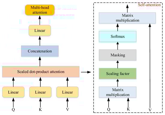
Figure 1.
Structure of the Transformer and the multi-head attention mechanism.
By introducing a gating mechanism, LSTM effectively alleviates the problems of gradient explosion and vanishing gradient faced by traditional recurrent neural networks (RNNs), thereby significantly improving the model’s processing effect on sequential data. The key structures of LSTM include the forget gate, input gate and output gate.
Firstly, in the forgetting stage, the forgetting gate combines the current input with the output of the previous moment and, through the activation function , determines with a certain probability which information in the cell state of the previous stage will be forgotten. The process is as follows:
where represents the forgetting gate, is the activation function, is the weight matrix of the forgetting gate, denotes the cell’s hidden state at timestep , is the corresponding state inherited from the previous timestep and is the bias term when the forgetting gate is in place.
Next, the input gate determines which new information to add to the cell state. The control signal generated by and the current candidate cell state generated by the tanh function will determine how much information to add to . After that, the cell state is updated with the following formula:
where is the weight matrix of the input gate, and are the bias terms at the time of the input gate and cell candidate, is the input gate, is the cell state at time and comes from the cellular state of the previous moment.
The last step reaches the output gate, which determines which information to output as the hidden state, and receives the of the previous state and the current state as input. The calculation formulas are as follows:
where is the weight matrix of the output gate and is the bias term when it is in the output gate. is the output gate.
As an extended form of LSTM, the implementation of BILSTM relies on two independent LSTM networks: forward LSTM processes data in sequence and captures historical information; backward LSTM reverse-processes sequences to extract future information, and compared with LSTM, it has a more comprehensive information processing capability. Figure 2 shows the BILSTM unit structure:
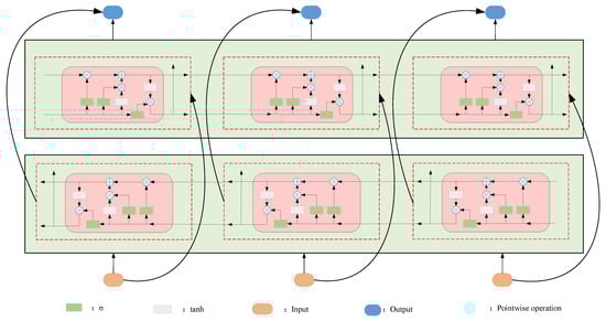
Figure 2.
Structure of BILSTM.
The output calculation formulas of BILSTM are as follows:
where represents the forward output result of LSTM, represents the reverse output result of LSTM, is the output of BILSTM at time , is the weight from the forward LSTM to the output and is the weight from the reverse LSTM to the output. represents the bias of the current output.
2.3. Improved Rime Ice Optimization Algorithm
The RIME (Rime Ice Optimization Algorithm), proposed by Su et al. [36] in 2023, comprises initialization, soft-rime search, hard-rime puncture, and positive greedy selection. However, random initialization lacks distributional control, leading to insufficient initial population diversity; the soft-rime search relies on uniform perturbations, making it hard to escape local optima in later stages; and the positive greedy update accelerates population convergence, weakening global exploration. To remedy these defects, this paper proposes the improved algorithm ORIME: a Sine–elite hybrid initialization ensures uniform coverage, the soft-rime stage is enhanced with Lévy flights to flee local optima, and the greedy update incorporates a roulette-wheel strategy to balance convergence and diversity.
2.3.1. Population-Initialization Improvements
Denote the entire population as . Each frost body is composed of frost ice particles , and each frost ice particle contains frost particles . Randomly initialize the population as follows:
where is the ordinal number of the frost body, is the ordinal number of the frost and ice particles, and is the QTH decision variable in the PTH candidate solution. Its position is updated as shown in Equation (18). and delimit the solution space, serving as its minimum and maximum bounds, respectively.
The Sine–elite hybrid initialization is used to initialize the population, and the mathematical expressions are as follows:
where represents the value at the current iteration step ; is the initial value, whose value is [0, 1]; is calculated from ; is the solution generated by the sine mapping; is a random number in the interval [−1, 1]; and is the solution generated by directional learning.
where represents the population position generated by the Sine–elite mixed initialization and is the fitness function.
2.3.2. Improvement of Search Strategies
To enhance the traversal ability of the soft frost search strategy in the global exploration stage, this paper introduces the Lévy flight mechanism to simulate the non-local and scale-free growth characteristics of soft frost particles. This mechanism generates a large jump step size through a double-tail distribution, thereby significantly enhancing the randomness and nonlinearity of the search path and effectively alleviating premature convergence. Based on this, the mathematical expression of the improved soft frost search strategy can be formalized as
where represents the updated position of the frost ice and is the position of the QTH frost ice of the optimal candidate solution. , and are random numbers in the interval [−1, 1]; denotes the present iteration count; represents the maximum number of iterations; [] indicates rounding off ; is a step function; is the coefficient of condensation; and are uniformly distributed random variables in the interval [0, 1]; is random numbers in the interval (1, 2]; takes 1.5; and is a vector operation.
The local development of the algorithm was carried out through hard frost puncture, as follows:
where is the updated position after hard frost puncture, is the standardized fitness value and is a random number in the interval [−1, 1].
The traditional soft frost particles mainly oscillate in small magnitudes around the historical optimal position, presenting obvious local aggregation characteristics. The introduction of the Lévy term enables particles to undergo long-distance transitions spanning multiple orders of magnitude in the early stages of iteration.
2.3.3. Improve the Positive Greed Mechanism
Based on the original positive greed mechanism, roulette selection is added. When the same optimal solution occurs five times in an iteration, the roulette mechanism comes into play, operating with a 30% probability of swapping, a 30% probability of flipping or a 40% probability of inserting patterns, aiming to enhance the quality of the global solution and the diversity of the population. The expression of the forward greedy selection mechanism is shown as follows:
where represents the position of the current solution and represents the position of the updated solution.
In roulette, represents the exchange probability, represents the flipping probability and represents the insertion probability. The mathematical expression is shown as follows:
where represents the optimal solution selected after roulette and represents the position after the roulette operation.
2.4. Full Text Framework
To estimate the SOH of NASA batteries, this paper proposes the ORIME–Transformer–BILSTM framework, with the process shown in Figure 3. The steps are as follows: First, clean the abnormal data and extract the multi-dimensional health factors of current, voltage and temperature; after the joint screening by Spearman and Kendall, the global features are extracted using the Transformer encoder and then input into BILSTM to capture the temporal evolution. The hyperparameters are optimized by ORIME during the training phase.
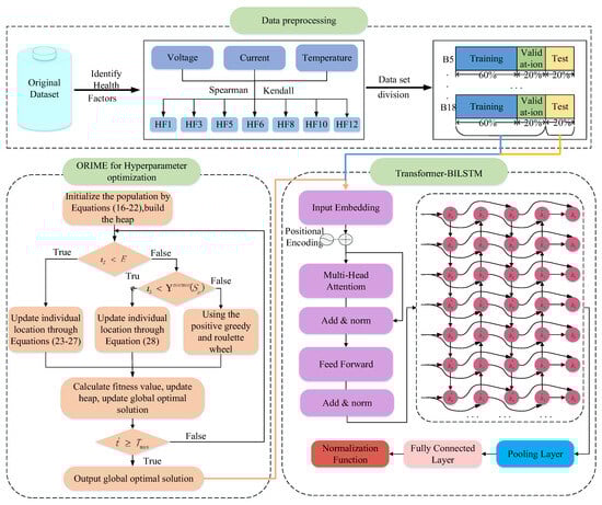
Figure 3.
Full-text Framework.
3. Experimental Preparation
3.1. Selection of the Dataset
This paper adopts the lithium-ion battery test dataset of NASA and selects four groups of batteries, namely B0005, B0006, B0007 and B0018 (denoted as B5, B6, B7 and B18 in the following text), all of which are of model 18650 and have a rated capacity of 2 Ah. Charging stage: The battery underwent constant-current (CC) charging at 1.5 A until its terminal voltage reached 4.2 V. Then, it was switched to constant pressure (CV) mode. After standing for a period of time, it entered the discharge stage: the battery was discharged at a constant 2 A until the voltage reached 2.7 V, 2.5 V, 2.2 V or 2.5 V, depending on the test condition. Figure 4a shows the voltage–current curves of the B5 cell during one charge–discharge cycle; Figure 4b presents the corresponding temperature profile.
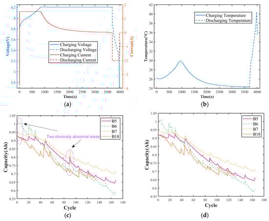
Figure 4.
One B5 cell cycle and Li-ion capacity fade: (a) voltage–current curve of the B5 cell during one charge–discharge cycle; (b) temperature profile; (c) raw capacity with outliers; (d) cleaned capacity trend.
In the battery dataset, some cycle periods show repetitive measurement data. To ensure the accuracy of the dataset, it was chosen to directly delete these duplicate data. Table 1 lists the locations where abnormal data occur in the NASA dataset.

Table 1.
Abnormal data deleted from the battery dataset.
The original capacity curve shown in Figure 4c has significant abnormal points due to reasons such as sensor drift and sudden changes in working conditions, which mask the true degradation pattern of the battery. After adaptive anomaly elimination and repair, the monotonic attenuation trend of capacity with the number of cycles was smoothly restored, as shown in Figure 4d.
3.2. Health Feature Extraction
As shown in Figure 5, Figure 5a,b show the charging curves of the B5 cell at the 10th cycle and every 30 cycles thereafter; Figure 5c,d present the corresponding discharging curves. As the number of cycles increases, the CC charging time of the battery gradually shortens, while the constant voltage charging time gradually extends. This phenomenon is in line with the trend of increasing internal resistance of the battery. Therefore, CC charging time (HF1) and constant voltage charging time (HF2) are taken as health factors to describe the health status of the battery. The isobaric rise charging time of lithium batteries is defined as the time required for the voltage to rise from low to high. Considering that batteries are rarely completely discharged in actual use, the time required for the voltage to rise from 3.9 V to 4.1 V is taken as HF3. During the CC charging process, the duration for which the current value remains at 1.5 A is significantly shortened. The time interval during the constant voltage charging stage when the current drops from 1.2 A to 0.6 A is selected as the health characteristic HF4. During the discharge stage, the time interval during which the discharge voltage drops from 3.8 V to 3.5 V is taken as the health characteristic HF5. The time it takes for the battery to reach the cut-off voltage becomes shorter and shorter, reflecting capacity attenuation. The time when the cut-off voltage occurs is taken as HF6. The peak temperature time during the charging stage is taken as HF7, the peak temperature time during the discharging stage as HF8, the maximum slope of the voltage curve during the charging stage as HF9, and the average discharge voltage during the discharging stage as HF10. As the number of charge and discharge cycles increases, in the CV stage, the area enclosed by the current curve from 1.5 A to 0.5 A and the time axis shifts to the left, and this area is taken as HF11. During the discharge stage, the discharge voltage on the voltage curve drops from 4.0 V to 3.2 V, and the area enclosed by the time axis is also changing. This area is taken as HF12.
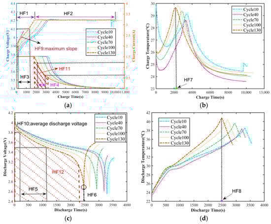
Figure 5.
Charging stage curve: (a) voltage, current; (b) temperature; discharge stage curve: (c) voltage; (d) temperature.
3.3. Screening of Health Factors
Given that the data on lithium battery degradation generally deviates from the normal distribution and the sample size is limited, this paper adopts a non-parametric filtering feature selection strategy and uses the Spearman and Kendall correlation coefficient methods to complete the double screening. The calculation formulas are as follows:
where is the Spearman correlation coefficient, and and are the average values of the health characteristic and the battery capacity sequence , respectively.
where represents the Kendall correlation coefficient, and and are the number of pairs with consistency and inconsistency in the corresponding features of the two groups, respectively.
The value range for both Spearman and Kendall is [−1, 1]. According to the value of the correlation coefficient, the correlation between features and SOH is classified into five levels: extremely strong, strong, medium, weak and very weak, as shown in Table 2 below.
Table 2.
Spearman and Kendall correlation grades.
Based on the calculation formulas of the Spearman and Kendall correlation coefficients mentioned above, the correlations between 4 battery samples and 12 health factors were quantitatively analyzed. The analysis results were presented in the form of a heat map, as shown in Figure 6.
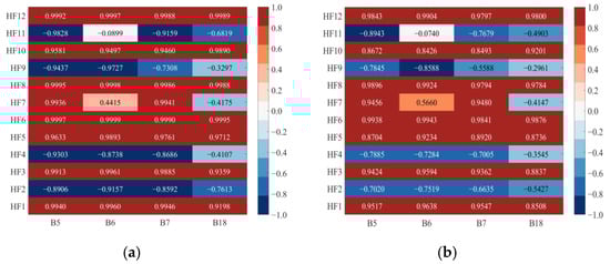
Figure 6.
Heat map of correlation coefficient: (a) Spearman; (b) Kendall.
In the data-driven method, the SOH estimation accuracy is significantly positively correlated with the quality of the input features. For this, health factors with a threshold greater than 0.8 are screened out in Spearman, and those with a threshold greater than 0.7 in Kendall. Figure 6a shows that the Spearman values between HF1, HF3, HF5, HF6, HF8, HF10, HF12 and all battery samples all exceed 0.8. Figure 6b further indicates that the absolute coefficients of the above seven factors in the Kendall test are all greater than 0.7. The consistency results of the two methods confirmed that the monotonic correlation strength reached the “extremely strong” level, so it was ultimately used as the model input.
The screened features have different dimensions. To avoid the features with larger dimensions dominating the prediction model and causing the model to be unstable, the Min–Max standardization method is adopted. All features are linearly transformed to the [0, 1] interval to eliminate the influence of dimensional differences while retaining the relative size relationship of the original data. The standardized formula is as follows:
where represents the standardized data, represents the original value, and and are the dataset’s minimum and maximum values, respectively
Based on the aforementioned feature screening framework, seven health factors were extracted from the NASA battery dataset and normalized to the interval [0, 1] by Min–Max. Figure 7 presents the normalized characteristic curves of four batteries over their complete cycle life. By comparison, it can be seen that the above seven factors all show a highly consistent monotonically decreasing trend with the capacity attenuation trajectory of the corresponding batteries, further verifying the rationality of using these selected factors for the SOH estimation of the batteries.
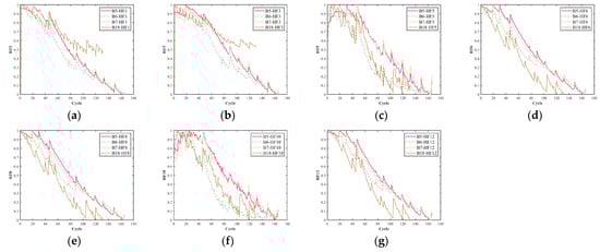
Figure 7.
Curves of the selected health factors: (a) HF1; (b) HF3; (c) HF5; (d) HF6; (e) HF8; (f) HF10; (g) HF12.
3.4. Dataset Division
To evaluate the model’s performance, we randomly split the original dataset into training, validation and test sets at a ratio of 6:2:2. The training set undertakes the function of parameter learning to train the model. The validation set monitors the effect in real time and is used to select the optimal hyperparameters and suppress overfitting. The test set assesses the model’s performance and verifies whether the final prediction results of the model meet expectations. By introducing a validation set, the training process of the model can be more accurately judged, and its performance can be estimated.
3.5. Model Parameter Configuration
The model training and data processing of the full text used Matlab2024a, the processor was an AMD Ryzen 7 6800H with Radeon Graphics 3.20 GHz, and the GPU was an NVIDIA GeForce RTX 3060 Laptop. For the convenience of comparison in the following text, the models used below are briefly remembered in sequence: Mark BP is denoted as M1, GRU as M2, LSTM as M3, BILSTM as M4, Transformer as M5, Transformer–BILSTM as M6, RIME–Transformer–BILSTM as M7, and ORIME–Transformer–BILSTM as M0. Table 3 shows the hyperparameter configuration of the model.
Table 3.
Hyperparameter configuration of the model.
4. Experimental Validation and Analysis
To systematically evaluate the performance of the M0 model, this paper designs three sets of progressive comparative experiments. Firstly, by using different proportions of training sets, the influence of changes in the amount of training data on the SOH prediction accuracy was explored. After that, a horizontal comparison was made between M0 and the seven models M1–M7. Finally, five methods reported in the literature from the past five years were selected and compared with M0 under the same small-sample scenarios to further verify the advancement and generalization ability of M0 in complex working conditions.
4.1. Performance Metrics
To rigorously benchmark the model’s predictive fidelity, we first adopt the canonical trio—Mean Absolute Error (MAE), Mean Absolute Percentage Error (MAPE) and Root Mean Square Error (RMSE)—whose minimization implies monotonically decreasing discrepancy between estimated and measured quantities. Complementing these staples, we further introduce two task-specific metrics: (i) the Error Dispersion Coefficient (EDC), which captures the stability of residuals across the operating envelope, and (ii) the Cross-Battery Consistency Index (CBCI), a dimensionless measure that gauges the transferability of learned representations among heterogeneous cells under disparate duty cycles. Collectively, the five indices provide a multi-faceted diagnostic of accuracy, robustness and generalizability. The mathematical formula of the evaluation indices are as follows:
where represents the sample size, and , and are the true value, predicted value and average value of the SOH, respectively. denotes MAE, MAPE, or RMSE.
4.2. The Prediction Effect of Different Training Set Ratios
To systematically evaluate the impact of the training set size on model performance, this paper divides the NASA battery B5, B6, B7 and B18 battery datasets into three partitioning schemes in chronological order: the first 40%, 50% and 60% of the data are taken as the training set, respectively; the middle 20% is used for validation; and the remaining part is used as the test set. Table 4 presents the SOH prediction errors under three division schemes.
Table 4.
Prediction errors under different training set ratios.
The results in Table 4 systematically reveal the influence law of the training set ratio on the accuracy of the prediction of remaining battery life, and further demonstrate the nonlinear threshold effect in the error convergence process. Overall, when the proportion of the training set increased from 40% to 60%, MAE, MAPE and RMSE all showed a monotonically decreasing trend on all four batteries, with average decreases reaching 18.9%, 20.3% and 21.4% respectively, significantly verifying the positive effect of data volume on the generalization ability of the model. By refining the proportion range of the training set and decomposing it into two stages, 40% to 50% and 50% to 60%, it can be clearly observed that the convergence rate is not constant. The initial increase from 40% to 50% generally yields the most significant performance gain, while the subsequent increase from 50% to 60% follows the principle of diminishing marginal returns, resulting in a slower rate of error reduction. Although the magnitude of average error reduction is substantial, the rate of average error reduction exhibits a minor dependence on the chosen battery, with a difference not exceeding 4%. This minor variation is attributed to the inherent heterogeneity of real-world battery data, where subtle differences in manufacturing and cycling history lead to unique degradation signatures. Crucially, the consistent monotonic downward trend observed across all four batteries confirms the model’s high robustness and its ability to generalize effectively even in the presence of individual sample variations. Furthermore, while the current results demonstrate performance potential, we acknowledge the importance of statistical rigor. Quantifying predictive uncertainty by calculating confidence intervals derived from several simulations for a given battery is a critical step for practical deployment and will be explicitly designated as a primary focus of our future work. Take the B5 battery as an example. When the proportion of the training set was increased from 40% to 50%, the MAE dropped from 0.3164% to 0.2819%, with a reduction rate as high as 10.9%. When the proportion of the training set further increased from 50% to 60%, the decline significantly narrowed to 8.2%. Similarly, the MAE of B7 batteries decreased by 6.8% during the 40% to 50% stage, while it only dropped by 6.4% during the 50% to 60% stage. The above results all point to a critical interval: when the proportion of the training set exceeds 50%, the marginal benefit of error improvement rapidly decreases, and the marginal improvement of MAE has shown a significant decreasing trend: the decline of the B5 battery in the 50–60% range further converges to 8.2%, and that of the B7 battery even drops to 6.4%. If the training data continues to be increased, the expected benefits will be further compressed, while the annotation cost will rise linearly.
A horizontal comparison further indicates that the smoothness of the battery capacity degradation curve and the noise level jointly determine the landing point of the “optimal” training ratio, rather than simply “the larger, the better”. Take the B18 battery as an example. Its degradation trajectory is extremely smooth, and the MAE can be reduced to 0.2281% under a 40% training set. If it is further expanded to 60%, although the relative decline is as high as 24.3%, the absolute error only drops by another 0.0554%, and the cost performance significantly declines, suggesting that the optimal sampling range can be locked between 40% and 50%. This sharp reduction in the rate of error improvement defines the onset of diminishing marginal returns for smooth sequences. On the contrary, due to the severe fluctuations in the later cycle, the MAPE of the B6 battery only decreased by 4.0% in the 40–50% stage and further dropped by 3.7% in the 50–60% stage. The overall convergence elasticity was the poorest. The noise amplified the dependence on the amount of training data, causing the threshold point to move forward and the convergence ceiling to be lower. It can be seen from this that if the training ratio of high-fluctuation sequences is less than 60%, the model has difficulty in fully capturing the degradation law, and the error remains at a high level. For battery B6, the error-reduction rate remains steep until the training-data share reaches 60%; beyond that point, each additional 10% of training data yields a relative gain of less than 1%. And 60% is precisely right after the inflection point of diminishing marginal returns. It can not only effectively suppress the uncertainty brought by noise but also avoid the economic inefficiency risks resulting from further expansion.
In conclusion, this paper uniformly adopts a 60% training set as the final configuration: this ratio is quantitatively confirmed to be the minimum required threshold that pushes all battery types, especially the most noise-affected sequences such as B6, past their critical convergence inflection point where the relative error-reduction rate drops below 4.0% per 10% increase in training data. While ensuring that all types of batteries approach their performance limits, it effectively avoids the low-efficiency investment brought about by subsequent expansion, achieving a global optimal trade-off between cost and accuracy.
4.3. Comparison with Different Models
To systematically evaluate the estimation performance of the proposed M0 model, this paper selects seven models from M1 to M7 as controls and completes the tests on a 60% training set. The prediction curves and relative error curves are shown in Figure 8 and Figure 9. The dotted line on the left indicates the starting position of the validation set of the data. The dotted line on the right represents the starting position of the test set prediction.
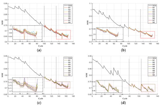
Figure 8.
SOH prediction result: (a) the prediction result of B5; (b) the prediction result of B6; (c) the prediction result of B7; (d) the prediction result of B18.
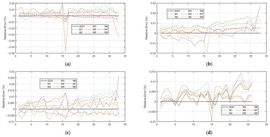
Figure 9.
SOH error comparison: (a) the prediction error of B5; (b) the prediction error of B6; (c) the prediction error of B7; (d) the prediction error of B18.
In Figure 8, the black solid line represents the true SOH value of the battery, while the solid lines of other colors correspond to the predicted curves of M1 to M7. To examine prediction quality across the entire lifespan in finer detail, we analyze the instantaneous relative error trajectory shown in Figure 9. This visualization reveals how the prediction error evolves throughout the battery’s lifetime, highlighting periods of optimal model performance and periods where error begins to accumulate. It should be noted that Figure 9 presents a deterministic view of error development for a single simulation run. Over most of the cycle life, the relative error remains stable and below five percent, rising only slightly as the battery approaches the end of life threshold at eighty percent state of health. This behavior is a common challenge in degradation modeling due to increasing nonlinearity. To further quantify the performance advantages of the M0 model, Table 5 presents the error values of each model.
Table 5.
Prediction errors under different models.
For the subsequent comparison, three metrics will be employed for evaluation: MAE, MAP and RMSE. The resulting EDC and CBCI values are listed in Table 6.
Table 6.
EDC and CBCI of all models on four batteries.
To evaluate the performance of various experimental models, we employed three error metrics: RMSE, MAPE and MAE. These indicators provide a comprehensive assessment of the differences between the predicted and actual values of the four test batteries at a temperature of 24 °C and a discharge current of 2 A. The results are summarized in Table 5, while Figure 8 shows the fitting curve and the visualization of the absolute error between the proposed model and the compared model. Based on the analysis in these charts, M0 demonstrates superior performance compared to other models in all error metrics. Firstly, in terms of MAE, the average MAE of M0 on the four batteries was 0.2374%, significantly lower than that of the other seven comparison models: 0.7975% for M1, 0.6969% for M2, 0.5581% for M3, 0.4747% for M4, 0.4370% for M5, 0.3478% for M6 and 0.2970% for M7. Compared with the suboptimal model M7, the MAE of M0 still achieves a relative gain of approximately 20.0404%. Compared with M1, which has the largest error, M0 reduces its MAE by 70.2401%, demonstrating a significant advantage in error compression. In terms of RMSE, the average value of M0 is 0.2761%, while that of M1 is as high as 1.2400%, M2 is 0.7881%, M3 is 0.6070%, M4 is 0.4860%, M5 is 0.4460% and M6 is 0.3728%. The average value of M7 is 0.3190%; M0 decreased by 13.4796% compared with M7 and by 77.7339% compared with M1. MAPE also maintained a comprehensive lead, with an average of 0.3563% for M0, 1.3040% for M1, 1.0470% for M2, 0.7910% for M3, 0.6200% for M4, 0.5770% for M5 and 0.4750% for M6. The average for M7 is 0.4070%. For the B6 battery with the most intense capacity fluctuations, the error advantage of M0 is further magnified: its MAE is only 0.2634%, a 71.4955% decrease compared to M1’s 0.9241%. The RMSE was only 0.3106%, a decrease of 69.3507% compared to M1’s 1.0134%. The MAPE was only 0.4337%, a decrease of 71.4934% compared to M1’s 1.5214%. All three indicators are significantly superior to the corresponding gap found for the smoothed degradation B18 battery, indicating that the robustness of M0 to high-noise conditions is nonlinearly amplified with the intensity of degradation fluctuations.
The coefficient of error dispersion (EDC) is defined as the ratio of RMSE to MAE. The closer the EDC is to 1, the more concentrated the error distribution is, and the fewer the extremely large errors are. A higher EDC indicates that the model is more sensitive to outliers and has poorer robustness. Further focusing on error coupling and stability reveals that M0 not only has a significant advantage at the mean level, but also has a significantly better ability to suppress extreme errors than the control group. Taking the B5 battery as an example, the error dispersion coefficient of M0 is 1.1936, which is lower than that of all control models. The coefficient of M1 is as high as 1.5045, meaning that for every 1% of the average deviation, there is approximately 1.5% of the potential extreme deviation. The coefficients of M2, M3 and M4 are 1.2524, 1.0646 and 1.1405, respectively. Analysis of the prediction results demonstrated that the instantaneous prediction error exhibited fluctuations across the testing cycles. Although they are better than M1, the standard deviations are all higher than 0.08, still revealing significant error fluctuations. Looking at the B6 battery, the error dispersion coefficient of M0 is 1.1807, which seems close to that of M3 at 1.0875. However, the MAE baseline of M3 is as high as 0.6503%, and its absolute fluctuation range is 0.3869 percentage points wider than that of M0. Although the coefficients of M5 and M6 on this battery are lower than 1.3, the MAE baselines reach 0.4233% and 0.3421%, respectively, which are significantly higher than those of M0, further weakening the robustness. The comparison of B18 batteries is more intuitive: The error dispersion coefficient of M0 is 1.2421, only slightly higher than that of M7 at 1.2188. However, the MAE of M7 at 0.2007% is still 16.2% higher than that of M0 at 0.1727%, indicating that even in the scenario of smooth degradation, M7 still has systematic bias. In summary, M0, with its dual advantages of a low error dispersion coefficient and a low standard deviation, compresses the average deviation while almost eliminating extremely large errors, laying a solid foundation for high-confidence SOH prediction intervals.
The Cross-Battery Consistency Index (CBCI) is defined as the difference between the maximum and minimum MAE values of the same model on four cells. The lower the CBCI, the narrower the error fluctuation of the model under different working conditions, and there is no need to readjust parameters for specific batteries during deployment. Cross-battery consistency analysis further revealed the working condition adaptability advantages of M0. Among the MAE results of the four batteries, the CBCI of M0 was only 0.0907 percentage points, significantly lower than that of M7 at 0.1086, M1 at 0.3412, M2 at 0.3254 and M3 at 0.2907. Further examination of the CBCI of MAPE revealed that M0 was 0.1826%, M7 was 0.2717%, and M1 was as high as 0.6786%. The CBCI of RMSE also shows that M0 is only 0.0836%, while M1 is 0.7712%. These data collectively indicate that the harsher the working conditions and the more intense the noise, the more significant the error advantage of M0. Its cross-battery consistency advantage provides solid data support for the large-scale application of diversified battery systems.
Based on the results in Table 5 and Figure 8, it can be seen that M0 leads comprehensively in terms of absolute accuracy, extreme error suppression and cross-cell robustness.
The superior performance of Model M0 over the control models stems from its specialized design, which explicitly addresses the inherent challenges of noise, nonlinearity and generalization in battery degradation data. Specifically, M0 integrates a multi-scale feature extraction module to enhance nonlinear mapping capabilities and employs a robust training objective to mitigate the impact of measurement noise. Its average MAE, RMSE and MAPE were only 0.2374%, 0.2761% and 0.3563% respectively, all significantly lower than those of all control models, and the error was compressed by more than 70% for the high-noise B6 battery. The error dispersion coefficient (EDC) consistently ranges from 1.18 to 1.24 and exhibits the minimum standard deviation observed, indicating that extreme errors have been effectively suppressed. The Cross-Battery Consistency Index (CBCI) has the lowest values for three indicators: MAE, RMSE and MAPE. During deployment, there is no need to re-tune parameters for specific cells, thus providing solid data support for large-scale, zero-parameter application of diverse battery systems.
4.4. Comparison with the Results of the Published Literature
To further verify the superiority of the method proposed in this paper, several representative methods from the recently published literature were selected for comparison. The SOH prediction model for lithium-ion batteries based on CPO-ELM-ABKDE in reference [37], the simple SOH estimation method based on constant voltage charging curve in reference [38], the SOH estimation method using IPSO-SVR dynamic hyperparameter optimization in reference [39], the SOH estimation method based on CNN–LSTM–Attention–FVIM in reference [40], and the algorithm of ion–FVIM fusing multiple health features and the SOH estimation method based on PSO-ELM fusing health indicators in reference [41] are denoted as M8, M9, M10, M11, and M12 in sequence. The RMSE and MAE results are recorded in Table 7.
Table 7.
Comparison of RMSE and MAE with recent representative methods.
The results in Table 7 show that M0 has the smallest error on all batteries and has a significant advantage over M8–M12. Measured by MAE, M0 is only 0.2537% in B5, approximately 0.67 times that of M8 and 0.50 times that of M11. The 0.2634% value obtained for B6 is approximately 0.46 times that of M10 and 0.73 times that of M12. The 0.2592% value obtained for B7 is approximately 0.59 times that of M8 and 0.72 times that of M12. The 0.1727% value obtained for B18 is only 0.20 times that of M8 and 0.34 times that of M11. RMSE is equally outstanding, with B5’s 0.2982% being approximately 0.47 times that of M8 and 0.34 times that of M9. The 0.3106% value obtained for B6 is approximately 0.29 times that of M8 and 0.53 times that of M10. The 0.2824% value obtained for B7 is approximately 0.58 times that of M8 and 0.38 times that of M11. The 0.2146% value obtained for B18 is only 0.18 times that of M8 and 0.37 times that of M10. Overall, M0 generally reduces errors to one-third to two-thirds of those of comparison methods in various indicators, demonstrating a significant performance advantage.
5. Conclusions
Aiming at the problems of single features of the model input and low estimation of a single model in the existing battery SOH estimation methods, an ORIME–Transformer–BILSTM model is proposed. Three types of health features regarding time, area and slope were extracted from the charge and discharge curves of NASA batteries. The features with stronger correlations were selected by using the Spearman and Kendall correlation coefficients. By using the Transformer module to capture the global dependency of batteries and combining it with BILSTM’s powerful processing capability for time series, the accuracy of the prediction of battery SOH has been significantly improved. Meanwhile, in order to reduce the uncertainty of manual parameter adjustment, ORIME is utilized to optimize the hyperparameters of the model. The experimental results show that the model proposed in this paper has higher prediction accuracy compared with other models. For example, on the NASA dataset, the MAE is within 0.2634% and the RMSE is below 0.3106; meanwhile, the EDC is within 1.2421%, and the CBCI of MAE and the CBCI of MAPE remain the lowest among all models, evidencing effective extreme-error suppression and consistent cross-battery reliability. Compared with several recently published approaches, M0 generally reduces errors to one-third to two-thirds of those of comparison methods across various indicators. Although some progress has been made in the research, there are still some directions that need further study, such as improving the input quality of data by using methods such as dimensionality reduction, denoising, and signal decomposition and further improvements in the algorithm to reduce running time. Crucially, future work will quantify prediction uncertainty via confidence intervals and, given current data limitations, expand validation beyond NASA to Oxford and CALCE repositories while incorporating temperature, partial-charge and irregular-cycling profiles for cross-chemistry robustness.
Author Contributions
Z.Z. (Zhiguo Zhao): Writing—Review and Editing, Methodology, Visualization. Y.D.: Software, Methodology, Conceptualization, Writing—Original Draft. K.L.: Software, Conceptualization, Writing—Review and Editing. Z.Z. (Zhirong Zhang): Software, Conceptualization, Writing—Review and Editing. Y.F.: Writing—Review and Editing, Supervision, Conceptualization. B.C.: Writing—Review and Editing. Q.Z.: Writing—Review and Editing, Supervision. All authors have read and agreed to the published version of the manuscript.
Funding
This work was supported by the Postgraduate Research & Practice Innovation Program of Jiangsu Province (SJCX25_2196) and the Doctoral Research Start-up Foundation by Huaiyin Institute of Technology (Z301B22530).
Data Availability Statement
The original contributions presented in the study are included in the article; further inquiries can be directed to the corresponding author.
Conflicts of Interest
The authors declare that they have no known competing financial interests or personal relationships that could have appeared to influence the work reported in this study.
References
- Waldmann, T.; Wilka, M.; Kasper, M.; Fleischhammer, M.; Wohlfahrt-Mehrens, M. Temperature dependent ageing mechanisms in Lithium-ion batteries–A Post-Mortem study. J. Power Sources 2014, 262, 129–135. [Google Scholar] [CrossRef]
- Qian, G.; Li, Y.; Chen, H.; Xie, L.; Liu, T.; Yang, N.; Song, Y.; Lin, C.; Cheng, J.; Nakashima, N.; et al. Revealing the aging process of solid electrolyte interphase on SiOx anode. Nat. Commun. 2023, 14, 6048. [Google Scholar] [CrossRef]
- Peng, Y.; Ding, M.; Zhang, K.; Zhang, H.; Hu, Y.; Lin, Y.; Hu, W.; Liao, Y.; Tang, S.; Liang, J.; et al. Quantitative analysis of the coupled mechanisms of lithium plating, SEI growth, and electrolyte decomposition in fast charging battery. ACS Energy Lett. 2024, 9, 6022–6028. [Google Scholar] [CrossRef]
- Krewer, U.; Röder, F.; Harinath, E.; Braatz, R.D.; Bedürftig, B.; Findeisen, R. Dynamic models of Li-ion batteries for diagnosis and operation: A review and perspective. J. Electrochem. Soc. 2018, 165, A3656. [Google Scholar] [CrossRef]
- Liu, W.; Xu, Y.; Feng, X. A hierarchical and flexible data-driven method for online state-of-health estimation of Li-ion battery. IEEE Trans. Veh. Technol. 2020, 69, 14739–14748. [Google Scholar] [CrossRef]
- Manfredi, P. Probabilistic uncertainty quantification of microwave circuits using Gaussian processes. IEEE Trans. Microw. Theory Tech. 2022, 71, 2360–2372. [Google Scholar] [CrossRef]
- Ma, B.; Yu, H.Q.; Wang, W.T.; Yang, X.B.; Zhang, L.S.; Xie, H.C.; Zhang, C.; Chen, S.Y.; Liu, X.H. State of health and remaining useful life prediction for lithium-ion batteries based on differential thermal voltammetry and a long and short memory neural network. Rare Met. 2023, 42, 885–901. [Google Scholar] [CrossRef]
- Xing, C.; Liu, H.; Zhang, Z.; Wang, J.; Wang, J. Enhancing Lithium-Ion Battery Health Predictions by Hybrid-Grained Graph Modeling. Sensors 2024, 24, 4185. [Google Scholar] [CrossRef]
- Kalhori, M.R.N.; Madani, S.S.; Fowler, M. Correlation-aware kernel selection for multi-scale feature fusion of convolutional neural networks in multivariate and multi-step time series forecasting: Application to Li-ion battery state of health forecasting. J. Energy Storage 2025, 139, 118860. [Google Scholar] [CrossRef]
- Li, N.; Zhang, H.; Zhong, J.; Miao, Q. SOH Estimation for Battery Energy Storage Systems Based-on Multi-scale Temporal Convolutional Network and Relaxation Voltage. IEEE Trans. Instrum. Meas. 2025, 74, 3555612. [Google Scholar]
- He, Z.; Gao, M.; Ma, G.; Liu, Y.; Chen, S. Online state-of-health estimation of lithium-ion batteries using Dynamic Bayesian Networks. J. Power Sources 2014, 267, 576–583. [Google Scholar] [CrossRef]
- Sun, H.; Sun, J.; Zhao, K.; Wang, L.; Wang, K. Data-driven ICA-Bi-LSTM-combined lithium battery SOH estimation. Math. Probl. Eng. 2022, 2022, 9645892. [Google Scholar] [CrossRef]
- Shi, D.; Zhao, J.; Wang, Z.; Zhao, H.; Wang, J.; Lian, Y.; Burke, A.F. Spatial-temporal self-attention transformer networks for battery state of charge estimation. Electronics 2023, 12, 2598. [Google Scholar] [CrossRef]
- Li, J.; Wang, X.; Tian, D.; Ye, M.; Niu, Y. A deep learning method based on transfer learning and noise-resistant hybrid neural network for lithium-ion battery state of health and state of charge estimation. Electrochim. Acta 2025, 543, 147577. [Google Scholar] [CrossRef]
- Zhang, Y.; Li, Z.; Kong, L.; Xu, H.; Shen, H.; Chen, M. Multi-step state of health prediction of lithium-ion batteries based on multi-feature extraction and improved Transformer. J. Energy Storage 2025, 105, 114538. [Google Scholar] [CrossRef]
- Zhang, L.; Wang, L.; Zhang, J.; Wu, Q.; Jiang, L.; Shi, Y.; Lyu, L.; Cai, G. Fault diagnosis of energy storage batteries based on dual driving of data and models. J. Energy Storage 2025, 112, 115485. [Google Scholar] [CrossRef]
- Huang, D.; Qin, M.; Liu, D.; Sun, Q.; Hu, S.; Zhang, Y. Multi-step ahead SOH prediction for vehicle batteries based on multimodal feature fusion and spatio-temporal attention neural network. J. Energy Storage 2025, 124, 116837. [Google Scholar] [CrossRef]
- Chen, T.; Zhang, C.; Jing, W.; Foo, E.Y.S.; Lai, X.; Zeng, N. State of Health Estimation for Lithium-Ion Batteries Using Separable LogSparse Self-Attention Transformer. IEEE Trans. Instrum. Meas. 2025, 74, 3522513. [Google Scholar] [CrossRef]
- Soon, K.L.; Soon, L.T. A hybrid quantum neural network and classical gated recurrent unit for battery state of health forecasting incorporating SHAP analysis. J. Energy Storage 2025, 136, 118596. [Google Scholar] [CrossRef]
- Song, J.; Wang, H.; Liu, Y.; Wang, R.; Wang, K. Enhancing variational autoencoder for estimation of lithium-ion batteries State-of-Health using impedance data. Energy 2025, 337, 138739. [Google Scholar] [CrossRef]
- Jin, M.; Ming, X.; Wei, D.; Qiao, Z.; Zhang, J.; Bai, X.; Qiu, P.; Wang, L. Physics-Informed Neural SOH Estimation Method for Lithium-ion Battery under Partial Observability and Sparse Sensor Data. 2025. Available online: https://sciety-labs.elifesciences.org/articles/by?article_doi=10.21203/rs.3.rs-6806872/v1 (accessed on 1 September 2025).
- Gou, B.; Xu, Y.; Feng, X. State-of-health estimation and remaining-useful-life prediction for lithium-ion battery using a hybrid data-driven method. IEEE Trans. Veh. Technol. 2020, 69, 10854–10867. [Google Scholar] [CrossRef]
- Miao, M.; Xiao, C.; Yu, J. Multi-source Domain Meta-learning Network for Battery State-of-Health Estimation under Multi-target Working Conditions. IEEE Trans. Power Electron. 2025, 40, 9786–9799. [Google Scholar] [CrossRef]
- Wu, M.; Xia, J. Meta-learning few-shot prediction of electric vehicle charging time with parallel CNN-Transformer networks. Int. J. Green Energy 2025, in press. [Google Scholar] [CrossRef]
- Meng, J.; Hu, D.; Lin, M.; Peng, J.; Wu, J.; Stroe, D.I. A domain-adversarial neural network for transferable lithium-ion battery state of health estimation. IEEE Trans. Transp. Electrif. 2025, 11, 7732–7742. [Google Scholar] [CrossRef]
- Li, X.; Yuan, C.; Wang, Z. Multi-time-scale framework for prognostic health condition of lithium battery using modified Gaussian process regression and nonlinear regression. J. Power Sources 2020, 467, 228358. [Google Scholar] [CrossRef]
- Zhang, C.; Tu, L.; Yang, Z.; Du, B.; Zhou, Z.; Wu, J.; Chen, L. A CMMOG-based lithium-battery SOH estimation method using multi-task learning framework. J. Energy Storage 2025, 107, 114884. [Google Scholar] [CrossRef]
- Yao, X.Y.; Chen, G.; Pecht, M.; Chen, B. A novel graph-based framework for state of health prediction of lithium-ion battery. J. Energy Storage 2023, 58, 106437. [Google Scholar] [CrossRef]
- Wang, T.; Dong, Z.Y.; Xiong, H. Adaptive multi-personalized federated learning for state of health estimation of multiple batteries. IEEE Internet Things J. 2024, 11, 39994–40008. [Google Scholar] [CrossRef]
- Chu, M.; Li, H.; Liao, X.; Cui, S. Reinforcement learning-based multiaccess control and battery prediction with energy harvesting in IoT systems. IEEE Internet Things J. 2018, 6, 2009–2020. [Google Scholar] [CrossRef]
- Liu, H.; Li, C.; Hu, X.; Li, J.; Zhang, K.; Xie, Y.; Wu, R.; Song, Z. Multi-modal framework for battery state of health evaluation using open-source electric vehicle data. Nat. Commun. 2025, 16, 1137. [Google Scholar] [CrossRef] [PubMed]
- Barragan-Moreno, A. Machine Learning-Based Online State-of-Health Estimation of Electric Vehicle Batteries: Artificial Intelligence Applied to Battery Management Systems. Master’s Thesis, Aalborg Universitet, Aalborg, Denmark, 2021. [Google Scholar]
- Wu, W.; Chen, Z.; Liu, W.; Zhou, D.; Xia, T.; Pan, E. Battery health prognosis in data-deficient practical scenarios via reconstructed voltage-based machine learning. Cell Rep. Phys. Sci. 2025, 6, 102442. [Google Scholar] [CrossRef]
- Kulkarni, S.V.; Arjun, G.; Gupta, S.; Sinha, R.; Shukla, A. Advanced battery diagnostics for electric vehicles using CAN based BMS data with EKF and data driven predictive models. Sci. Rep. 2025, 15, 32848. [Google Scholar] [CrossRef]
- Zhang, K.; Tang, L.; Fan, W.; He, Y.; Rao, J. Aging and echelon utilization status monitoring of power batteries based on improved EMD and PCA of acoustic emission. IEEE Sens. J. 2024, 24, 12142–12152. [Google Scholar] [CrossRef]
- Su, H.; Zhao, D.; Heidari, A.A.; Liu, L.; Zhang, X.; Mafarja, M.; Chen, H. RIME: A physics-based optimization. Neurocomputing 2023, 532, 183–214. [Google Scholar] [CrossRef]
- Yan, M.X.; Deng, Z.H.; Lai, L.; Xu, Y.H.; Tong, L.; Zhang, H.G.; Li, Y.Y.; Gong, M.H.; Liu, G.J. A Sustainable SOH Prediction Model for Lithium-Ion Batteries Based on CPO-ELM-ABKDE with Uncertainty Quantification. Sustainability 2025, 17, 5205. [Google Scholar] [CrossRef]
- Zhang, Q.; Chen, X.; Cai, Y.; Qin, T. A Simple Method for State of Health Estimation of Lithium-ion Batteries Based on the Constant Voltage Charging Curves. Electrochemistry 2024, 92, 077008. [Google Scholar] [CrossRef]
- Shang, S.; Xu, Y.; Zhang, H.; Zheng, H.; Yang, F.; Zhang, Y.; Wang, S.; Yan, Y.; Cheng, J. Enhancing Lithium-Ion Battery State-of-Health Estimation via an IPSO-SVR Model: Advancing Accuracy, Robustness, and Sustainable Battery Management. Sustainability 2025, 17, 6171. [Google Scholar] [CrossRef]
- Liu, G.; Deng, Z.; Xu, Y.; Lai, L.; Gong, G.; Tong, L.; Zhang, H.; Li, Y.; Gong, M.; Yan, M.; et al. Lithium-ion battery state of health estimation based on CNN-LSTM-Attention-FVIM algorithm and fusion of multiple health features. Appl. Sci. 2025, 15, 7555. [Google Scholar] [CrossRef]
- Chen, J.; Liu, Y.; Yong, J.; Yang, C.; Yan, L.; Zheng, Y. State of health estimation of lithium-ion batteries using fusion health indicator by PSO-ELM model. Batteries 2024, 10, 380. [Google Scholar] [CrossRef]


Disclaimer/Publisher’s Note: The statements, opinions and data contained in all publications are solely those of the individual author(s) and contributor(s) and not of MDPI and/or the editor(s). MDPI and/or the editor(s) disclaim responsibility for any injury to people or property resulting from any ideas, methods, instructions or products referred to in the content. |
© 2025 by the authors. Licensee MDPI, Basel, Switzerland. This article is an open access article distributed under the terms and conditions of the Creative Commons Attribution (CC BY) license (https://creativecommons.org/licenses/by/4.0/).