Abstract
To address the challenges of large-scale production data, complex temporal dynamics, and the difficulty in extracting key reservoir performance indicators, this study proposes an intelligent time-series analytics approach, validated using an offshore oilfield case. The methodology integrates a cascaded outlier detection framework combining the 3-Sigma rule and the One-Class Support Vector Machine (OC-SVM). The 3-Sigma rule is first used for rapid statistical screening of extreme outliers, followed by OC-SVM for nonlinear anomaly detection, enhancing the accuracy of dynamic production data preprocessing. Key indicators—including initial production capacity, decline rate, water-cut trend, and recoverable reserves—are automatically extracted through hybrid modeling combining production decline analysis and waterflood characteristic curves. Algorithm reliability is rigorously evaluated using error metrics (SSE: Sum of Squared Errors, MSE: Mean Squared Error, MAE: Mean Absolute Error, RMSE: Root Mean Squared Error) and goodness-of-fit (R2). Experimental results demonstrate that the proposed method outperforms manual extraction, achieving <10% error in daily oil production and waterflood performance curve fitting, while significantly enhancing accuracy and automation. This framework provides a robust data−driven foundation for intelligent reservoir management.
1. Introduction
Reservoir development has gradually advanced into the era of fine-scale and intelligent management. The massive influx of production dynamic data has revealed the inefficiency and poor adaptability of traditional analysis methods that heavily rely on human expertise. Moreover, various development indicators exhibit complex characteristics over time, including nonlinearity, multi-scale variability, and strong noise, all of which further complicate the extraction of critical information. Therefore, it is imperative to develop an intelligent and efficient data processing and indicator extraction algorithm that can automatically identify and distill key development features embedded in time series data, thereby supporting reservoir production analysis and decision-making.
In response to this challenge, numerous studies have been conducted by domestic and international researchers. Traditional industrial practices typically involve the use of waterflood characteristic curves, production decline analysis, and injection-production ratio combined with pressure dynamic interpretation. For example, in 2006, Lin ZhiFang and his team proposed the application of waterflood characteristic curves and analyzed how common techniques such as layered development, infill drilling, and fracturing influence these curves [1]. In 2010, Nie Renshi studied the application of natural energy indicators in waterflood dynamic analysis, finding that the ratio between average formation pressure drop and the dimensionless elasticity production index can accurately predict oil recovery efficiency. Combined with waterflood characteristic curves, this method helps determine reasonable cumulative and staged injection-production ratios [2]. In 2022, Sun Zhaole proposed a reservoir parameter inversion method based on early production decline analysis, effectively addressing the production instability issues caused by operational changes in the early stages of well production [3].
Time series analysis has significant implications for interpreting production data in reservoir engineering. In 2001, Professor Bernhard Schölkopf of AT&T Labs proposed the One-Class Support Vector Machine (OC-SVM) method, which has since found broad application in outlier detection of reservoir time-series data [4]. In 2004, Wang Xuezhong developed a method for staging multilayer sandstone reservoirs based on time series data such as recoverable reserves and production rates in Gudong Oilfield. In 2024, Zuo Yi utilized time series data during numerical simulation of layered fault blocks in Gangdong Block II to support the division of reservoir development and evaluation stages [5]. Additionally, preprocessing of outliers in production dynamic data is essential. The widely adopted 3-sigma rule, introduced by Walter in the early 20th century, has been widely accepted in petroleum engineering.
Despite the various methods proposed for indicator extraction from time series data, current approaches struggle to perform real-time analysis amid the growing scale of digital oilfields, where each well generates large volumes of dynamic production data. As reservoirs mature, production data tend to exhibit strong nonlinearity and phase transitions, rendering traditional manual methods inefficient, highly subjective, and unsuitable for the demands of intelligent management. To address these limitations, this study adopts a hybrid approach that leverages OC-SVM and 3-sigma statistical principles to detect and process outliers in production dynamics using machine learning and statistical theory. Based on this cleaned time series data, production decline models (harmonic, hyperbolic, exponential) and waterflood characteristic curves (types A, B, C, and Zhang’s type) are applied to automatically extract key development indicators. This method significantly improves the efficiency and intelligence of key indicator extraction and holds great promise for supporting intelligent reservoir management.
2. Methods for Handling Anomalies in Production Dynamic Data
To eliminate anomalies in production dynamic data, this study applies both the One-Class Support Vector Machine (OC-SVM) and the 3-Sigma method to process time-series production data. Furthermore, to reduce volatility in the dataset, monthly production averages are computed and adjusted accordingly.
To systematically evaluate the applicability and effectiveness of an intelligent time-series-based extraction method for key development indicators, this study employs producing well groups from an offshore oilfield with phased commissioning as empirical research subjects. A multidimensional analytical framework was constructed to conduct systematic statistical analysis and comparative validate.
2.1. One-Class SVM for Machine Learning-Based Outlier Detection
The One-Class Support Vector Machine (OC-SVM) is a single-class learning method based on the theory of Support Vector Machines (SVMs), primarily used in anomaly detection, noise reduction, and small-sample learning scenarios. Unlike traditional binary SVMs, OC-SVMs are trained using only positive samples. The goal is to learn the distribution of normal data and establish a decision boundary that encloses the majority of the samples, enabling classification of new, potentially anomalous data points.
Mathematically, OC-SVM utilizes kernel functions to map input data into a high-dimensional feature space, where it seeks to separate the data from the origin and maximize the margin between them as shown in (1). The optimization problem is formulated to tolerate a certain degree of outliers while identifying a hyperplane that best contains the training data. Commonly used kernel functions include the Radial Basis Function (RBF), polynomial, and sigmoid kernels, with the RBF kernel being most prevalent due to its strong non-linear mapping capabilities [6]. In this study, the Radial Basis Function (RBF) kernel was selected primarily due to its four significant advantages. Firstly, the RBF kernel possesses strong nonlinear mapping capabilities, which can effectively map data with complex nonlinear distributions in low-dimensional spaces to high-dimensional feature spaces. This perfectly adapts to the complex distribution characteristics of the data in this research, providing a more accurate basis for boundary division for the model. Secondly, it only requires the optimization of one core parameter (γ). Compared with multi-parameter kernel functions such as polynomial kernels and sigmoid kernels, it significantly reduces the difficulty of parameter tuning and computational costs, facilitating the rapid realization of model optimization. Thirdly, the RBF kernel is less sensitive to data scales. After basic normalization, it can effectively weaken the interference caused by differences in the scales of different features, enhancing the robustness of the model in diverse data scenarios. In addition, it can flexibly balance local fitting and global generalization capabilities through the parameter γ. It can not only capture the core distribution characteristics of the data but also avoid overfitting to training noise, enabling the model to maintain stable generalization performance on unknown data, which is highly consistent with the requirements of this research for model reliability and adaptability.
In this equation, x denotes the test sample, xi represents the training samples, αi are the support vector coefficients, is the kernel function, and is the bias term. A major advantage of OC-SVM is its capability to handle datasets containing only one class of observations while maintaining strong generalization ability. In this study, OC-SVM is employed to detect and eliminate outliers from high-dimensional geological data in oil reservoirs. As illustrated in Figure 1, OC-SVM is particularly well-suited for handling non-linear reservoir characteristics. Red dots represent anomalous samples (outliers), and blue dots represent normal samples. OC−SVM uses a high−dimensional hyperplane to separate the two types of samples, thus achieving anomaly detection. However, it requires significant computational resources, is sensitive to hyperparameter tuning, and its performance may be affected by the quality of input data [7].
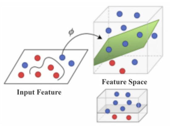
Figure 1.
Hyperplane classification using OC-SVM.
2.2. 3-Sigma Statistical Method for Outlier Detection
The 3-Sigma Rule is a well-established empirical technique in statistics, commonly used for anomaly detection under the assumption of a normal distribution. For normally distributed random variables, approximately 99.73% of the values fall within the range of ±3 standard deviations () from the mean (), as shown in Figure 2. Data points that fall outside this range are considered anomalies see (2).
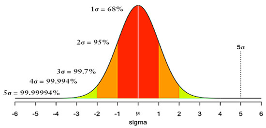
Figure 2.
Distribution curve illustrating the 3-Sigma Rule.
In the equation, denotes the observed sample value, is the mean of the sample, and is the standard deviation.
The 3-Sigma method is advantageous for its simplicity and robustness, particularly in datasets that approximate a normal distribution. In this study, it is used alongside OC-SVM to detect extreme fluctuations in well production data, thereby enhancing data quality and ensuring the accuracy and stability of subsequent modeling efforts [8].
2.3. Combined Anomaly Detection Workflow (3-Sigma + OC-SVM)
In this study, a cascaded anomaly detection strategy was implemented to improve the robustness and efficiency of production data preprocessing. The workflow first applies the 3-Sigma statistical rule to remove obvious outliers that deviate significantly from the normal distribution, providing a coarse-level screening of the dataset. Subsequently, the One-Class Support Vector Machine (OC-SVM) is applied to the filtered data to capture potential nonlinear or hidden anomalies in high-dimensional feature space.
This sequential combination effectively balances computational cost and detection precision: the 3-Sigma rule ensures rapid anomaly identification, while the OC-SVM refines the detection by learning the intrinsic structure of the remaining data. The hybrid approach also mitigates the sensitivity of OC-SVM to extreme noise and reduces overfitting risks in large-scale production datasets.
2.4. Conversion to Monthly Production Data
Daily production data are the most direct indicators of reservoir performance. However, as shown in Figure 3a, daily production values for a single well are often subject to significant variability due to operational timing and external factors [9]. To mitigate these fluctuations, this study adopts a monthly averaging approach Figure 3b, using monthly average values to represent well performance. For wells that did not operate at full capacity throughout the month, actual operational time is taken into account, and oil and fluid production are adjusted accordingly to better reflect true well capacity. The conversion is based on (3), where denotes monthly full-capacity oil production, is daily oil production, is operational time, and is the number of days in the month.
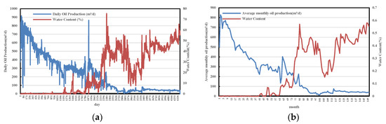
Figure 3.
Comparison of oil production data before and after conversion. (a) BlockP-A01 Daily oil production. (b) Monthly oil production after adjustment.
3. Key Indicator Extraction Methods
3.1. Development Stage Classification
Water cut is one of the most critical dynamic parameters in reservoir development. Its classification not only aids in identifying the stages of reservoir development and the advancement of waterflooding but also provides a data foundation for injection-production analysis, water control strategies, residual oil tapping, and refined production management. Therefore, establishing a scientifically sound classification scheme for water cut is fundamental for efficient and refined reservoir management [10].
In this study, the water cut is divided into five stages: Water-free (fw < 2%), Low water cut (2% < fw < 20%), Medium water cut (20% < fw < 60%), High water cut (60% < fw < 90%), and Ultra-high water cut (fw > 90%). As illustrated in Figure 4, this five-stage classification provides higher resolution than traditional three-stage methods. It improves the precision in characterizing production water behavior and better supports the needs of high-resolution reservoir dynamic analysis, enabling more accurate extraction of time-dependent development indicators.
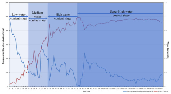
Figure 4.
Water cut stage classification diagram.
3.2. Production Decline Analysis
Production decline is a fundamental reflection of reservoir performance over time. Time series–based decline models can not only accurately simulate actual production behavior but also be used to forecast future productivity and ultimate cumulative oil production. By intelligently identifying decline types and estimating model parameters, precise classification of development stages and automatic extraction of key indicators can be achieved—thereby offering strong technical support for dynamic reservoir management [11].
In this study, after classifying production periods by water cut, each stage is fitted using exponential, harmonic, and hyperbolic decline models. Table 1 above summarizes the basic characteristics, governing equations, and expressions for ultimate cumulative oil production. Here, is the initial production rate, is the initial decline rate, is production time, is cumulative oil production, is the maximum recoverable oil, and n is the decline exponent.

Table 1.
Decline model relationships.
By comparing model fitting performance, the most suitable decline model is selected to determine the production decline rate. Based on an economic production limit, the ultimate cumulative oil production during a well’s life cycle or production stage can be predicted [12].
3.3. Waterflood Characteristic Curves
For reservoirs that have entered high or ultra-high water cut stages, waterflood characteristic curves are widely used in practical applications. By modeling the relationships between oil, water, and total fluid production, these curves can be used to predict cumulative oil production and water cut progression. Common curve types include Type A, B, C, and D, each governed by distinct empirical Equations (4) to (7), which quantitatively link water cut and cumulative oil production [13].
However, each curve type corresponds to only a specific shape of the fw–R* relationship. Their expressions are often complex, and parameters can be difficult to estimate, making them less suitable for automated workflows. This study adopts the Zhang-type waterflood characteristic curve in (8), which integrates the features of various traditional types while maintaining mathematical simplicity and practical utility [14]. In this equation, is cumulative water production, is cumulative oil production, Lp is cumulative liquid production, and , are fitting coefficients.
The waterflood characteristic curve is a well-established method for estimating recoverable and economically recoverable reserves. For Types A–D, a typical maximum water cut of 98% is assumed to determine ultimate recoverable oil from (9) to (16). In these, is ultimate recoverable reserves, fw is water cut, is the limiting water cut, R is the water–oil ratio, is the liquid–oil ratio, and a1–a3, b1–b3 are fitting parameters.
The Zhang-type curve supports two alternative formulations for estimating cumulative oil production (17) and (18), using fitting coefficients a, b, c, time t, and water cut fw. By introducing a limiting water cut (typically 98%), it can also estimate ultimate recoverable reserves. In reservoirs with complex geological conditions, Zhang’s model offers superior fitting accuracy compared to traditional types [15].
4. Verification Methods for Indicator Extraction Reliability
To quantitatively assess the accuracy of the extracted development indicators, this study introduces five commonly used error evaluation metrics: SSE (Sum of Squared Errors); MSE (Mean Squared Error); MAE (Mean Absolute Error); RMSE (Root Mean Squared Error); R2 (Coefficient of Determination). The mathematical definitions of these metrics are presented in (19) to (23).
The use of these five metrics allows for a comprehensive, multi-angle evaluation of the model’s performance in terms of both precision and robustness. Specifically: SSE reveals the overall magnitude of error, MSE and RMSE reflect the sensitivity to large deviations, MAE accounts for the average deviation in a stable manner, R2 measures the goodness-of-fit of the model. By jointly applying these evaluation indices, the model’s reliability can be scientifically verified across different dimensions, ensuring the credibility and stability of the extracted indicators.
5. Results Analysis
To verify the applicability and effectiveness of the proposed time series–based intelligent extraction method for key development indicators, this study applies it to multiple production wells from an actual offshore oilfield. The analysis covers wells from different commissioning batches, well types, and water cut stages. Extracted indicators are statistically evaluated and compared to explore dynamic patterns and demonstrate the algorithm’s technical workflow, as illustrated in Figure 5.
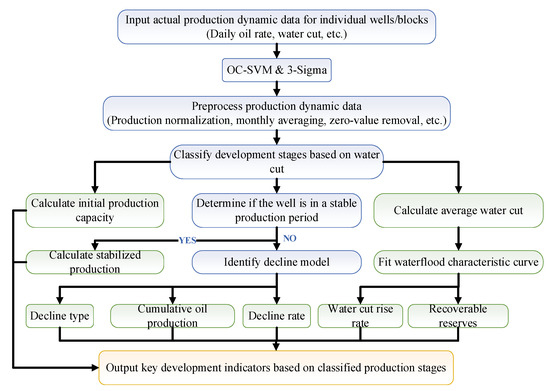
Figure 5.
Technical workflow for intelligent indicator extraction.
The process begins by collecting well/block-level production dynamic data such as daily oil rate and water cut. After data preprocessing—including outlier removal and monthly averaging—the production data are classified into five stages based on water cut: water-free (fw < 2%), low (2% < fw < 20%), medium (20% < fw < 60%), high (60% < fw < 90%), ultra-high (fw > 90%). Subsequently, decline models and waterflood characteristic curves are fitted within each stage to extract key indicators such as water cut rise rate and recoverable reserves.
5.1. Outlier Analysis
In reservoir development, raw production data often contain anomalies due to measurement errors, equipment faults, or human intervention. These outliers—such as abrupt spikes, discontinuities, or zero values—can distort production trends, interfere with decline curve fitting, and reduce the accuracy of key indicator extraction.
This study combines the OC-SVM machine learning approach with the 3-sigma statistical method to develop a robust outlier identification and correction framework tailored to time-series features. This significantly improves the accuracy of decline model and waterflood curve fitting. In practical implementation, the proposed cascaded framework first applied the 3-Sigma rule for rapid removal of statistically extreme values, and then employed the OC-SVM to identify nonlinear anomalies in the residual dataset. Figure 6 illustrates the effect of outlier removal for both daily oil production and monthly fluid production in the BlockP. By eliminating extreme spikes and valleys, the reconstructed data show smoother temporal trends while preserving the underlying production behavior. The optimized curves better represent actual reservoir dynamics and form a reliable foundation for subsequent model fitting and indicator computation.
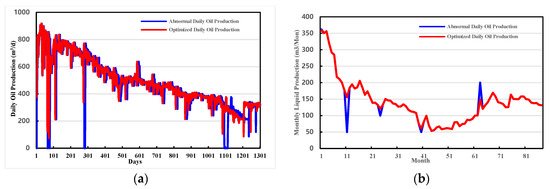
Figure 6.
Stage-wise decline curve fitting: A case study of BlockP-D25. (a) Daily oil production after outlier removal. (b) Monthly liquid production after outlier removal.
5.2. Indicator Extraction Analysis: Decline Rate, Cumulative Oil Production, and Model Comparison
This section presents a systematic analysis of the key development indicators extracted using the proposed method, focusing on decline rate, water cut rise rate, and single−well recoverable reserves.
- (1)
- Analysis of Decline Rate and Cumulative Oil Production
Due to the complexity of production profiles across the life cycle of a well, three classic decline models—exponential (n = 0), hyperbolic (0 < n < 1), and harmonic (n = 1)—are used for curve fitting (as listed in Table 1), based on Q–t, Np–t, and Np–Q relationships.
As shown in Figure 7, for BlockP-D25, the hyperbolic decline model achieved the best fitting performance during both low and medium water cut stages, with R2 values of 0.936 and 0.929, respectively. This model can therefore be used to predict stage-wise ultimate production, offering valuable reference for development strategy and reserves evaluation.
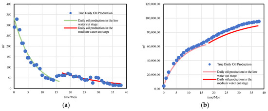
Figure 7.
Example: BlockP-D25 well. (a) Stage-wise daily production fitting. (b) Stage-wise cumulative oil fitting.
- (2)
- Analysis of Water Cut Rise Rate and Recoverable Reserves
To assess waterflood efficiency at different stages, the water cut rise rate (fw) is used as a sensitivity indicator. A predictive model for single-well recoverable reserves is constructed based on waterflood characteristic curves and fitting parameters a3 and b3, incorporating a limiting water cut of 95% to estimate NR.
Taking BlockP-D25 as an example, the average water cut rise rate during the low and middle water cut stages is 1.40 and 1.48, respectively (see Figure 8), and the final estimated recoverable reserves are 377,000 m3. These results demonstrate the method’s reliability for phase-specific analysis and precise recovery evaluation.
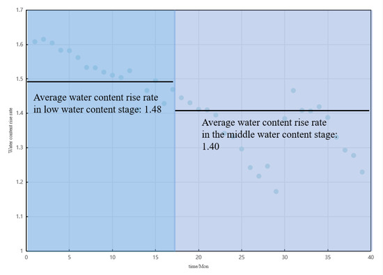
Figure 8.
Water cut rise rate (fw) per stage: BlockP-D25 well.
Additionally, to better quantify the dynamics of water advancement, a new indicator—the rise rate of water cut (Rfw)—is introduced, defined as the incremental change in water cut over time in (24). This parameter serves as a sensitive measure of the reservoir’s displacement front and waterflood progression.
- (3)
- Model Comparison and Waterflood Curve Optimization
To enhance the accuracy of water cut rise rate and reserves prediction, this study compares three waterflood characteristic curve models: Type A, B, and C. Regression is performed using logarithmic relationships between fw and Np, as shown in (24) to (26).
Statistical results summarized in Table 2 show that the Type C model offers the highest fitting accuracy, with R2 > 0.95 for 433 wells—significantly outperforming Type A (140 wells) and Type B (15 wells). Figure 9 shows the comparison results for well BlockP-D25. The Type C model achieved an R2 of 0.943 and yielded predictions closely aligned with observed data.
Table 2.
Model fitting accuracy for three waterflood types.
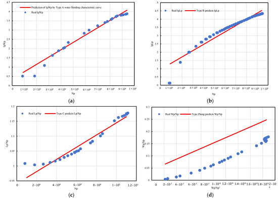
Figure 9.
Fitting comparison of four waterflood characteristic curves (A–C, Zhang−type) for BlockP-D25 (a). Type A; (b). Type B; (c). Type C; (d). Type Zhang.
5.3. Reliability Verification
To confirm the reliability of the proposed time series–based indicator extraction algorithm, this section presents a multi-angle validation using error analysis, model fitting quality, and manual benchmark comparisons.
- (1)
- Validation of Outlier Detection Method
After implementing the proposed outlier handling workflow, fitting accuracy significantly improved. In BlockP wells, post-processed data more closely followed physical reservoir behavior. As seen in Figure 10, the model curve fluctuations decreased, peak distortions were removed, and core trends were preserved.
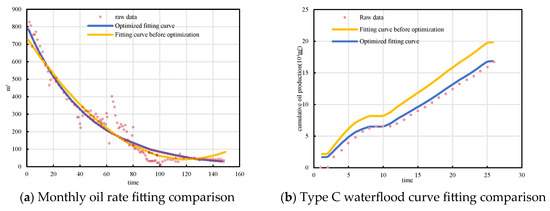
Figure 10.
Reliability verification of outlier processing algorithm.
In addition, errors in key indicators (such as decline rate, water cut rise rate, initial production) dropped from 20–60% to within 5%. Table 3 shows the before-and-after results for several wells. Notably, some unrealistic values (e.g., extremely high water cut rise rates or negative decline rates) were corrected to physically reasonable ranges.
Table 3.
Before-and-after comparison of outlier-corrected indicators.
Large−scale indicator comparison verifies the algorithm stability, and statistical comparisons are conducted on more than 40 wells and 6 types of key indicators; multiple bar graphs clearly show the significant differences in indicators before and after outlier processing and the fluctuation compression effect; especially in highly sensitive scenarios such as low water content stage and early production capacity prediction, the optimized data results are more credible [16].
- (2)
- Validation of Indicator Extraction Accuracy
To evaluate the effectiveness and reliability of the proposed time series–based method for extracting key reservoir development indicators, a comprehensive validation was conducted from multiple perspectives. This included statistical error analysis, model fitting accuracy assessment, and comparative validation against manually calibrated benchmarks [17].
Comparing the processing results of several representative well points it can be seen in Figure 11 that all indicators fall within the allowable error range, among which RMSE is generally less than 1%, and MSE is stable within 0.05, reflecting high prediction accuracy and data consistency. The statistical results in the figure also show that the optimized extraction value is better than that before abnormal data processing in terms of average level and variance control, further improving the stability of the model [18].
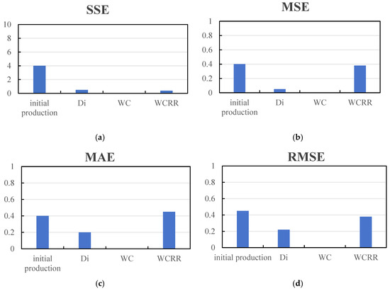
Figure 11.
Accuracy measurements. (a) SSE (Sum of Squared Errors); (b) MSE (Mean Squared Error); (c) MAE (Mean Absolute Error); (d) RMSE (Root Mean Squared Error).
To further verify the practical applicability of the algorithmic model, a comparative analysis was conducted between manually calibrated indicators and automatically extracted results for selected representative wells [19]. Corresponding waterflood characteristic curves were also plotted. As shown in Figure 12, Figure 13 and Figure 14, the model-derived results closely matched the manually interpreted benchmarks in both shape and trend. The average deviation was less than 10%, and the coefficient of determination (R2) was consistently greater than 0.98. Notably, for sensitive indicators such as decline rate, initial production capacity, and economic limit water cut, the algorithm maintained excellent error control. The fitted curves exhibited smooth and continuous trajectories without abnormal fluctuations or mismatches, further confirming the robustness and reliability of the proposed method [20].
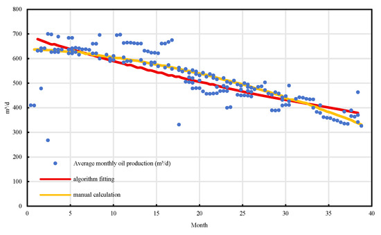
Figure 12.
Average monthly oil production fitting of well BlockP-A17.
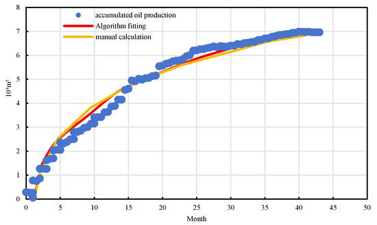
Figure 13.
Predicted cumulative oil production of well BlockP-A17.
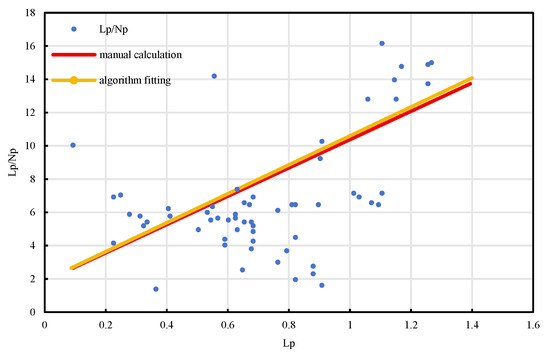
Figure 14.
BlockP-A17 Well Lp/Np.
Through a comprehensive validation involving multiple wells, multiple indicators [21], and multiple evaluation dimensions [22,23], the results demonstrate that the intelligent extraction method proposed in this study exhibits excellent consistency, stability, and physical plausibility [24]. The automatically extracted results closely match those obtained through manual interpretation, indicating the method’s potential to serve as a reliable substitute for human judgment [25]. Various statistical indicators confirm that the model outputs are stable and the errors are well-controlled, thereby providing a robust foundation for the construction of large-scale automated analytical workflows [26].
First, error analysis comparing extracted indicators with manually calculated values shows that the SSE, MSE, MAE, and RMSE for all indicators remain at low levels—significantly below the commonly accepted thresholds in typical engineering applications. Specifically, the MSE values for initial production capacity, decline rate, water cut, and water cut rise rate are all below 0.5; MAE values are also less than 0.5; and RMSE values are consistently under 1 [27]. These results confirm that the extracted development indicators are both accurate and stable [28].
Furthermore, comparative validation using actual well production data was conducted. Taking Well A17 from a representative offshore oilfield as an example, the study fitted and analyzed multiple indicators, including average monthly oil production, daily production decline rate, Lp/Np ratio, water cut rise rate, and cumulative oil production [29]. The comparison results reveal that the dynamic production curves fitted by the automated algorithm closely align with those derived from manual calculations, with absolute errors generally within 10%, thereby confirming the consistency between the extracted indicators and actual reservoir behavior [30]. Among them, the Lp/Np ratio and the daily oil production decline curves demonstrated particularly strong fitting performance [31], effectively capturing production attenuation and waterflooding dynamics, which further substantiates the reliability of the proposed algorithmic model [32].
6. Conclusions
This study addresses the challenges of significant fluctuations in production data and low efficiency in extracting key indicators during the reservoir development process. A time series–based intelligent extraction and prediction algorithm for reservoir development indicators is proposed and implemented. Using a real offshore oilfield block with 467 production wells (including 75 horizontal wells and 392 directional wells) as a case study, the applicability and effectiveness of the method were systematically validated.
For data preprocessing, a cascaded anomaly detection workflow combining the 3-Sigma rule and the One-Class SVM was employed. The 3-Sigma rule was first used for coarse screening of abnormal data, followed by OC-SVM for fine detection of nonlinear anomalies, which significantly improved data smoothness and modeling accuracy. Building on this, an automated extraction model for key development indicators was constructed, focusing on seven core metrics such as initial production capacity, decline rate, water cut, and recoverable reserves. The method utilizes production decline models (exponential, harmonic, and hyperbolic) and waterflood characteristic curves (Types A, B, and C) to perform intelligent segmentation and parameter fitting across the production lifecycle.
Model validation results demonstrate that the proposed algorithm achieves high predictive accuracy and strong stability. All fitted curves yielded coefficients of determination (R2) exceeding 0.9, with prediction errors generally below 10%. Notably, the fitting error of the Type C waterflood curve decreased by approximately 90% after outlier removal compared to untreated data. Furthermore, comparative analysis across different well types and development batches revealed that infill wells exhibited significantly higher decline rates than primary wells, and horizontal wells showed higher decline rates than directional wells—further confirming the model’s adaptability and accuracy under diverse field conditions.
In summary, the proposed time series–based intelligent extraction and forecasting method significantly enhances the efficiency and precision of dynamic data analysis in oilfield development. It provides reliable support for evaluating the performance of large-scale well clusters and optimizing production strategies, demonstrating strong potential for practical engineering applications.
Author Contributions
L.Q.: Investigation, supervision, writing—original draft; L.C.: data curation, methodology; Z.D.: formal analysis, visualization; C.L.: validation, writing—original draft; L.C.: investigation, resources; Y.D.: validation, writing—review and editing; Q.C.: methodology, writing—review and editing; W.X.: visualization, writing—original draft; F.M.: writing—original draft; Z.W.: funding acquisition, project administration, supervision, writing—review and editing. All authors have read and agreed to the published version of the manuscript.
Funding
This research was funded by National Natural Science Foundation of China grant number 52104018, 52104017, and 52274030.
Data Availability Statement
The data presented in this study are available on request from the corresponding author.
Conflicts of Interest
Authors Ling Qiu, Zupeng Ding, Chuan Lu, Long Chen, Qinwan Chong and Yintao Dong were employed by the CNOOC Research Institute Co., Ltd. The remaining authors declare that the research was conducted in the absence of any commercial or financial relationships that could be construed as a potential conflict of interest.
Abbreviations
| SVM | Support Vector Machine |
| SSE | Sum of Squared Errors |
| MSE | Mean Squared Error |
| MAE | Mean Absolute Error |
| RMSE | Root Mean Squared Error |
| RBF | Radial Basis Function |
References
- Lin, Z.; Yu, Q.; Zhao, M. Research on problems in the application of waterflood characteristic curves. Pet. Explor. Dev. 1986, 5, 37–44. [Google Scholar]
- Sun, Z.; Cheng, L.; Jia, P.; Jin, Z.; Zhang, X. Reservoir parameter inversion method based on early production decline analysis of oil wells. Spec. Oil Gas Reserv. 2022, 29, 101–106. [Google Scholar]
- Nie, R.; Jia, Y.; Shen, N.; Qin, X.; Zhang, W.; Liu, S. Application of natural energy indicators in water injection dynamic analysis. Xinjiang Pet. Geol. 2010, 31, 174–177. [Google Scholar]
- Cheng, X. Discrimination and processing of abnormal environmental air monitoring data at natural gas production sites. Energy Conserv. 2022, 6, 169–171. [Google Scholar]
- Schölkopf, B.; Platt, J.C.; Shawe−Taylor, J.; Smola, A.J.; Williamson, R.C. Estimating the support of a high−dimensional distribution. Neural Comput. 2001, 13, 1443–1471. [Google Scholar] [CrossRef]
- Li, Q. Discrimination and processing of abnormal monitoring data at natural gas production sites. In Proceedings of the 31st National Natural Gas Academic Annual Meeting, Hefei, China, 30 October 2019; Volume 06: Storage and Transportation, Safety, Environmental Protection, and Comprehensive Topics, pp. 299–302. [Google Scholar] [CrossRef]
- Zuo, Y.; Song, J.; Shi, Z.; Qiao, J.; Zu, X.; Zheng, J. Modeling algorithms and case studies of reservoir development stages. Xinjiang Pet. Geol. 2024, 45, 118–125. [Google Scholar]
- Qian, J.; Liu, F.; Li, D.; Jin, X.; Li, F. Large−scale KPI anomaly detection based on ensemble learning and clustering. J. Cybersecur. 2020, 2, 157. [Google Scholar] [CrossRef]
- Gao, N. Study and countermeasures of production decline law of Sabai expansion wells. West. Prospect. Eng. 2024, 36, 58–60. [Google Scholar]
- Jin, Q. Oil Well Production Prediction Method and Application Based on Data−Driven and Waterflood Characteristic Fusion. Master’s Thesis, China University of Petroleum (Beijing), Beijing, China, 2023. [Google Scholar] [CrossRef]
- Zhang, J. A simple and practical waterflood characteristic curve. Pet. Explor. Dev. 1998, 3, 72–73. [Google Scholar]
- Liang, G.; Liu, Y.; Xie, Q.; Xia, Z.; Liu, S.; Zhou, J.; Bao, Y. Physical simulation and improved numerical simulation method of non−condensable gas co−injection in SAGD process. In Proceedings of the SPE Asia Pacific Oil and Gas Conference and Exhibition, Jakarta, Indonesia, 10–12 October 2023; SPE: Dallas, TX, USA, 2023; p. D031S020R003. [Google Scholar]
- Conde, M.P.; Teixeira, P.R.F.; Didier, E. Numerical simulation of an oscillating water column wave energy converter: Comparison of two numerical codes. In Proceedings of the ISOPE International Ocean and Polar Engineering Conference, Maui, HI, USA, 19–24 June 2011; p. ISOPE−I−11−328. [Google Scholar]
- Li, Y.; Chen, B.; Lai, G. Numerical simulation of wave forces on seabed pipeline by finite element and LES. In Proceedings of the ISOPE International Ocean and Polar Engineering Conference, Honolulu, HI, USA, 25–30 May 1997; p. ISOPE−I−97−194. [Google Scholar]
- Olarewaju, J.S. Application of numerical simulation, flowmeter analysis and conditional simulation for modeling dual−permeability reservoirs. In Proceedings of the SPE Middle East Oil and Gas Show and Conference, Manama, Bahrain, 15–18 March 1997; p. SPE−37727−MS. [Google Scholar]
- Akbar, A.M.; Arnold, M.D.; Harvey, A.H. Numerical simulation of individual wells in a field simulation model. Soc. Pet. Eng. J. 1974, 14, 315–320. [Google Scholar] [CrossRef]
- Cao, X.; Sun, J.; Qin, F.; Ning, F.; Mao, P.; Gu, Y.; Li, Y.; Zhang, H.; Yu, Y.; Wu, N. Numerical analysis on gas production performance using a multilateral well system in Shenhu area. Energy 2023, 270, 126690. [Google Scholar] [CrossRef]
- Xu, Y. Implementation and Application of the Embedded Discrete Fracture Model (EDFM) for Fractured Reservoirs. Ph.D. Thesis, The University of Texas at Austin, Austin, TX, USA, 2015. [Google Scholar]
- Zhang, R.; Jia, H. Production prediction for waterflood reservoirs using multivariate time series and VAR models. Pet. Explor. Dev. 2021, 48, 175–184. [Google Scholar] [CrossRef]
- Zhang, H.; Guo, J.; Zhang, T.; Haoran, G.; Chi, C.; Shouxin, W.; Tang, T. Numerical study of wall−retardation effects on proppant transport in rough fractures. Comput. Geotech. 2023, 159, 105425. [Google Scholar]
- Wang, H.; Mu, L.; Shi, F.; Dou, H. Oil production forecasting in ultra−high water−cut stages based on recurrent neural networks. Pet. Explor. Dev. 2020, 47, 1009–1015. [Google Scholar] [CrossRef]
- Yang, Y. Progress in big data and AI applications in Shengli Oilfield exploration and development. Pet. Geol. Recovery Eff. 2022, 29, 1–10. [Google Scholar]
- Zhang, H.; Xiao, Z.; Zhao, J.; Shitao, C.; Chenjun, Z.; Bo, W.; Li, H. Coupled numerical simulation of electric and fluid fields during SC−CO2 displacement using digital rocks. In Proceedings of the SPWLA Annual Logging Symposium, Dubai, Saudi Arabia, 17–21 May 2025; p. D041S015R001. [Google Scholar]
- Yin, L.; Jiafang, X.; Chen, M.; Wang, S.; Du, Q.; Zhou, Q.; Qi, X.; Zhang, G. A new approach integrating geomechanics and numerical simulation for fracture prediction in buried hills. In Proceedings of the SPWLA Annual Logging Symposium, Dubai, Saudi Arabia, 17–21 May 2025; p. D051S022R003. [Google Scholar]
- Zhang, L.; Dou, H.; Wang, T.; Wang, H.; Peng, Y.; Zhang, J.; Liu, Z.; Mi, L.; Jiang, L. Single−well production prediction in waterflood oilfields using an integrated temporal convolutional neural network model. Pet. Explor. Dev. 2022, 49, 996–1004. [Google Scholar] [CrossRef]
- Pan, H.; Liu, J.; Gong, B.; Zhu, Y.; Bai, J.; Huang, H.; Fang, Z.; Jing, H.; Liu, C.; Kuang, T.; et al. Construction and preliminary application of a large−scale dynamic analysis model for reservoirs. Pet. Explor. Dev. 2024, 51, 1175–1182. [Google Scholar] [CrossRef]
- Liu, X.; Li, Q.; Li, N.; Chen, W.; Dai, Z. Numerical simulation of acid flow in rough fractures. SPE J. 2025, 30, 3009–3028. [Google Scholar] [CrossRef]
- Li, Q.; Teng, B. Rapid numerical simulation of heat transfer in fractured geothermal reservoirs. SPE J. 2025, 30, 3029–3047. [Google Scholar] [CrossRef]
- Yang, F.; Du, X.; Lu, D. Coupled numerical simulation of physicochemical processes for CO2 storage in depleted reservoirs. SPE J. 2025, 30, 3165–3188. [Google Scholar] [CrossRef]
- Chen, W.; Zhao, M.; Cai, M.; Pan, H.; Ni, T.; Luo, B. Quantitative evaluation of waterflooding performance using indicator−feature models. Acta Pet. Sin. 2016, 37, 80. [Google Scholar]
- Ren, Y.; Liu, Y.; Hou, Y.; Wang, G.; An, Y. Intelligent fine waterflooding of multilayer offshore sandstone reservoirs based on machine learning. Sci. Technol. Eng. 2023, 23, 14183–14191. [Google Scholar]
- Delgado-Torres, C.; Donat, M.G.; Gonzalez-Reviriego, N.; Caron, L.-P.; Athanasiadis, P.J.; Bretonnière, P.-A.; Dunstone, N.J.; Ho, A.-C.; Nicoli, D.; Pankatz, K.; et al. Multi-model forecast quality assessment of CMIP6 decadal predictions. J. Clim. 2022, 35, 4363–4382. [Google Scholar] [CrossRef]


Disclaimer/Publisher’s Note: The statements, opinions and data contained in all publications are solely those of the individual author(s) and contributor(s) and not of MDPI and/or the editor(s). MDPI and/or the editor(s) disclaim responsibility for any injury to people or property resulting from any ideas, methods, instructions or products referred to in the content. |
© 2025 by the authors. Licensee MDPI, Basel, Switzerland. This article is an open access article distributed under the terms and conditions of the Creative Commons Attribution (CC BY) license (https://creativecommons.org/licenses/by/4.0/).