Abstract
Global electric vehicle sales are growing exponentially, with the European Union actively promoting the adoption of electric vehicles to significantly reduce mobility-related emissions. Concurrently, research efforts are increasingly directed toward optimizing vehicle charging strategies for the effective integration of renewable energy sources. Nevertheless, despite extensive theoretical studies, few practical implementations have been carried out. In response, this paper presents a digital twin of a microgrid designed specifically for optimizing the charging schedules of an electric vehicle fleet, with the goal of maximizing photovoltaic self-consumption. Machine learning algorithms are utilized to forecast vehicle energy consumption, and various heuristic optimization methods are applied to determine optimal charging schedules. The system incorporates an interactive dashboard, enabling users to input specific preferences or delegate charging decisions to a real-time optimizer. Additionally, a user-centric decision support system was developed to provide recommendations on optimal vehicle connection timings and heat pump setpoints. Certain algorithms failed to converge on a feasible optimal solution, even after 340 s and over 500 generations, particularly within high-production scenarios. Conversely, using the GWO-WOA algorithm, optimal charging schedules are computed in less than 25 s, balancing photovoltaic power exports under varying weather conditions. Furthermore, K-Means was identified as the most effective clustering technique, achieving a Silhouette Score of up to 0.57 with four clusters. This configuration resulted in four distinct velocity ranges, within which energy consumption varied by up to 5.8 kWh/100 km, depending on the vehicle’s velocity. Finally, the facility managers positively assessed the usability of the DT dashboard and the effectiveness of the decision support system.
1. Introduction
The transport sector is the second-largest source of GHG emissions globally, accounting for 23% of CO2 emissions in the world [1]. To reduce emissions, the European Union (EU) is promoting the electrification of mobility, offering various incentives to potential buyers [2]. However, such environmental benefits would only originate from electric vehicles (EVs) if the sources of electricity used for charging were based on renewable energy sources (RESs), like solar and wind power. Moreover, such electrification of mobility poses some challenges, even from the perspective of the electric system, as the demand for electricity increases and requires adequate infrastructure for charging. At the same time, this electrification also leads to opportunities for grid balancing by integrating EVs with RESs, since EVs can act as flexible loads or storage devices that can respond to the fluctuations in the supply and demand of electricity [3]. For example, EVs can charge during periods of excess RES production (grid to vehicle) and discharge during a shortage (vehicle to grid). In this way, the variability and intermittency of RESs will be smoothed out for better integration into the electric system. In this context, technologies such as digital twins (DTs), digital and synchronized replicas of real systems [4], and energy management systems [5] are increasingly applied to microgrids to optimize their operation.
In the field of microgrids, significant attention has been devoted to developing algorithms for optimizing EV charging in microgrids [6,7]. The need to integrate EVs into the existing power grids with minimal environmental impacts has driven such sudden interest in innovation. A notable example of this trend is [8], where the authors developed a model for optimizing the charging schedules of battery electric vehicles. The model, adapted to consider the different environmental impacts of the generation mix, demonstrates the substantial reduction in GHG emissions made possible by smart charging strategies. In a different approach, Bao et al. [9] presented a methodology for mixed fleet scheduling of airport ground service vehicles that considers both fuel-based and electric tractors in the fleet. Another critical contribution is presented by Yin et al., who introduced a methodology for the safe and efficient operation of electrical grids using the optimum scheduling strategy of EVs [10]. Their methodology included ML models such as Long-Short Term Memory (LSTM) and XGBoost combined with the CPLEX solver to handle complex optimization problems. Ahmadi and Shiradi [11] analyzed distribution networks with high EV penetration, applying different meta-heuristic optimization algorithms to residential and non-residential EV users. Their results demonstrated that smart charging could mitigate or eliminate blackouts and voltage violations. Fresia et al. [12] investigated an industrial microgrid within a renewable energy community, where company cars and delivery trucks were used as mobile storage. Their multi-objective optimization revealed that following only the desired power exchange profile resulted in a self-sufficiency rate of 56.43%, while simultaneously increasing operating costs. Similarly, Nguyen and Nguyen [13] proposed a hybrid PSO–GWO algorithm to minimize losses and improve load balancing. Their results confirmed that the hybrid approach outperformed single algorithms in loss and voltage optimization.
Advanced algorithms can be implemented in real-time, enabling management of all energy flows, such as EV charging, grid interaction, and heat pump operations, to reduce energy drawn from the grid. Examples are found in the work of Mathur et al. [14] and Uzair et al. [15], which present a relevant example of real-time operational optimization. In ref. [16], an alternative optimization method was proposed by the authors using Multi-Agent Deep Reinforcement Learning. With appropriate management of EVs and PVs, grid energy consumption could be reduced by up to 40%, compared to multi-home systems that do not participate in energy trading or incorporate EVs. In ref. [17], a multi-objective optimal charging strategy was presented, aimed at peak load shaving and developed using various optimization algorithms. DTs are also proving to be effective tools for enabling real-time energy management. Li and Xu [18] developed a DT of two smart houses incorporating an LSTM model for building load forecasting and different optimization algorithms for reducing energy costs while maintaining user satisfaction. Their results indicated that LSTM achieved an MAPE of 4.4%, while an improved WOA outperformed other heuristic algorithms such as particle swarm optimization. Similarly, Benedetto et al. [19] demonstrated that a vehicle-to-building DT can reduce demand charges and partially substitute stationary storage systems.
The rapid expansion of EV adoption requires parallel research efforts: on the one hand, reducing emissions associated with EV charging; on the other, accurately characterizing RES forecasts and EV consumption. As shown by Menyhart [20], even hybrid vehicles can provide additional flexibility and value to the grid, as evidenced by a one-year analysis of hybrid vehicle operation. Ref. [21] presented CALNet, a hybrid LSTM–CNN-based method for accurately forecasting RES generation in microgrids. Zhao et al. [22] have proposed XGBoost and Light GBM-based approaches for the forecast of the remaining driving range based on an extensive EV database: NDANEV. Although these models achieved very good accuracy, they include a large number of features, such as braking ratio, acceleration ratio, and motor and battery output energy, which makes them difficult to replicate in simpler scenarios. On the other hand, H.A. Yavasoglu et al. [23] proposed a range estimation method for EV using data gathered and experimentation. They used a Decision Tree to identify road type and an ANN to predict range based on variables such as HVAC usage, vehicle weight, traffic, and road type. Their model resulted in an accuracy of more than 94%. Though these models are very efficient, the replicability by non-experts or people with less sophisticated equipment is limited.
Research Gaps and Novel Contributions
Overall, the reviewed studies underscore the growing importance of ML and optimization algorithms in balancing EV charging demands with grid stability. However, as also noted by Almeida et al. [24], a critical gap remains in the deployment of these approaches in real-world case studies, highlighting the need for further development tailored to actual user requirements. This observation is consistent with the studies summarized in Table 1, where only 12% of the works were implemented in real-case applications. Therefore, the main gaps identified in the current literature can be summarized as follows:
- Although numerous studies address EV charging and microgrid optimization, only a limited number are implemented in real-world case studies and operated in real-time.
- In the few real implementations available, user interaction is often overlooked; facility manager preferences are rarely incorporated, and existing tools can be too complex for practical use.
- There is limited deployment of DTs for smart grids that simultaneously integrate EVs, buildings, and PV systems.
- Methodologies for estimating individual EV consumption based solely on simple data collection remain scarce.
This work aims to address the gaps encountered in the literature by presenting a DT that integrates ML models and optimization algorithms capable of real-time response. This article is distinguished from previous studies by five main contributions:
- A replicable DT architecture based entirely on open-source tools and designed to optimize EV charging using simple yet effective algorithms.
- The DT recommends EV charging strategies according to user preferences and integrates adaptive machine learning models calibrated for each vehicle.
- Continuously improving consumption models, enabled by real-time synchronization of data between the physical and virtual layers;
- The implementation and operation of a real-life case study involving a fleet of EVs.
- An interactive DT dashboard that is intuitive for facility managers and capable of providing real-time recommendations to enhance overall system efficiency.

Table 1.
Overview of the state of the art and paper contribution.
Table 1.
Overview of the state of the art and paper contribution.
| Ref. | System Type | Real Case Study | Real-Time Synchronization | Digital Twin | EV Consumption Modeling | User Interaction | Optimization Approach |
|---|---|---|---|---|---|---|---|
| [6] | Microgrid | Yes | HiGHS and SNOPT solvers | ||||
| [7] | Microgrid | Newton-based optimization | |||||
| [8] | National grid | n.d. | |||||
| [9] | Microgrid | Yes | ALNS, MSILS, CPLEX, iALNS | ||||
| [10] | Microgrid | LSTM and XGBoost for EVs charging load | n.d. | ||||
| [11] | Distribution network | Yes | DHLO, GWO, PSO | ||||
| [12] | Microgrid | Yes | Matlab R2022b (Gurobi solver) | ||||
| [13] | Microgrid | PSO, GWO, PSO–GWO hybrid | |||||
| [14] | Microgrid | Yes | Biogeography-Based Optimization | ||||
| [15] | Building with PV | Yes | Yes | Yes | TOPSIS, MCE, PROMETHEE | ||
| [16] | Microgrid | Average consumption | Multi-agent DDPG | ||||
| [17] | Regional distribution network | RBH-PSO, PSO | |||||
| [18] | Two houses | n.d. | Yes | Yes | IWOA, WOA, PSO, DEA, Dragonfly | ||
| [19] | Microgrid | Yes | Yes | n.d. | |||
| [21] | Microgrid | Yes | No (CALNet, CNN, and LSTM for RESs) | N/A | |||
| [22] | EV | XGBoost, LightGBM | N/A | ||||
| [23] | EV | Yes | ANN, Decision Tree | N/A | |||
| This study | Microgrid | Yes | Yes | Yes | K-Means, Agglomerative, Gaussian Clusterings | Yes | GWO-WOA. IGWO, CGO, GA, NSGA-II |
This methodology was applied in the framework of the DigiBUILD project [25]. Precisely, a DT was developed to optimize the management of the microgrid associated with Emotion S.r.l. (Perugia, Italy), an Italian company operating in the field of EV charging stations. This case study focuses on one of the company’s buildings, which is equipped with 50 kWp PV panels and four EV charging points, each rated at 11 kW. Through the use of optimization algorithms, charging strategies will be provided via the DT for the company’s fleet of EVs. The algorithm’s input will include forecasts of building energy consumption, PV production, and user needs. Moreover, the DT can control the charging of connected EVs in real-time, leveraging available PV power to reduce energy costs. This will contribute not only to energy efficiency but also to grid stability. Finally, the DT dashboard not only displays historical and real-time information but also serves as a decision support system (DSS), suggesting manual actions such as setting the setpoint temperature for HVAC and advising on connecting or disconnecting vehicles. An overview of the DT is presented in Figure 1, which includes a high-level scenario diagram. The physical twin encompasses all the energy systems involved in the microgrid, as well as the metering systems. An interconnection layer regulates the input and output between the digital and physical twins, ensuring the update of the models and their impact on the physical twin through APIs. Real-time synchronization between the physical system and the digital twin is achieved via Apache Kafka topics, which stream sensors and operational data directly to the DT in real time. Historical and semantic information is stored and accessed via a data warehouse and an intelligent querying mechanism [26]. Finally, the facility manager interacts with the digital twin to monitor the system and optimize EV charging thanks to all the models included in the digital twin back-end. The presented approach meets the most up-to-date focus in scientific literature data and adaptive control for the optimal use of energy in facilities hosting RESs and EV fleets [27].
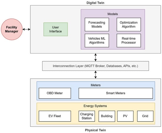
Figure 1.
Scenario diagram of the proposed microgrid digital twin framework.
2. Materials and Methods
The DT developed in the context of this work presents various models that interact with each other, as anticipated in Figure 1 and detailed in Figure 2. The models of the DT of this study, white boxes in Figure 2, are focused on three different types of algorithms:
- ML models, for each vehicle, which are used to estimate EV-specific consumption based on average trip velocity;
- An optimization algorithm designed to determine optimal strategies based on different self-consumption objectives and user preferences;
- A real-time processor employed to optimally control charging and provide recommendations.

Figure 2.
Digital twin architecture of this work.
Figure 2.
Digital twin architecture of this work.

Regarding the ML models, an algorithm is executed monthly to update clustering models based on historical vehicle data. Once updated, the user can access the DT dashboard to run the optimization and input preferences, such as the required vehicles, time of need, distance to be traveled, and expected average speed. The last two pieces of information are used by the pre-trained models to calculate specific energy consumption and, consequently, the energy required by each selected vehicle.
For the optimization algorithm, the energy required by each vehicle is used to determine the minimum State of Charge (SoC) necessary at the specified time. While user preferences are not strictly essential for the algorithm, the algorithm’s essential inputs include the SoC of each vehicle at the start of the optimization process and forecasts of PV production and building consumption for the next 24 h. Specifically, forecasts of PV production and building electricity consumption were not developed as part of this study, since they had already been provided by the project framework. This forecasting procedure selects the best-performing model from a trained ensemble of Random Forest Regressor, Gradient Boosting Regressor, Lasso Regressor, and Multilayer Perceptron models. The input data includes the building’s and EV chargers’ historical electricity consumption, PV generation, and historical and forecasted weather variables. Once the forecasted data is available, the optimization process begins, and it provides the user with three different strategies based on the level of self-consumption they wish to achieve.
Through the DT dashboard, the user can select one of the suggested strategies or activate the “Automatic Control” mode, which engages the real-time processor module. The output of each strategy specifies the optimal time to connect the EV for charging, as well as the power modulation behavior for each charging port. The system then regulates the charging power at each port, ensuring the predicted balance between energy import and export. In the “Automatic Control” mode, if the real-time data processor detects an imbalance in grid power import or export, the algorithm automatically adjusts the charging power or provides suggestions to address the issue, functioning as a DSS.
2.1. Optimization Algorithm
The optimization algorithm developed in this study aims to address a question often noted in the literature: the balance between PV production, building consumption, and electricity consumption for EV charging. Given the practical nature of this study, the end-user was consistently considered to ensure that the findings could be applied tangibly through the DT. Consequently, the optimization problem includes various constraints that account for both user preferences and physics-based relationships.
This algorithm aims to exploit various strategies for effectively charging 10 EVs. It involves forecasting the next 24 h of PV production (EPV), building energy consumption (EB), and estimating grid energy purchase (Ebuy) and potential energy sales (Esell). Other inputs are the real-time vehicle SoCs and user energy requirements (calculated by vehicle models and user preferences). Finally, the 240 decisional variables of this problem are the energy demanded for charging vehicle in hour ().
The optimization problem includes seven different constraints, which comprise both linear and non-linear equations, as well as those based on if-else statements or comparisons between variables. This was made possible by using Python 3.12 as a development environment for the optimization problem, ensuring both a smooth integration into the DT and interaction between different models through the use of Application Programming Interfaces (APIs).
The first constraint is applied to incorporate user preferences. Based on the machine learning (ML) model trained for each vehicle and the user inputs, the required SoC, , and the specified time of use are implemented using Equation (1). Specifically, between the time of optimization ( = 1) and the time of use, , the sum of the energy consumed by vehicle in each hour must be greater than or equal to the energy required to reach the desired SoC. This energy is calculated as the difference between the SoC at the time of the optimization run , gathered in real time, and , multiplied by the capacity of vehicle and charging efficiency .
For each vehicle :
Secondly, the operational constraints regarding the charging limits are implemented through Equations (2) and (3). For each hour , the sum of must be lower than the maximum total plug capacity (44 kW). Simultaneously, the values of higher than zero in each hour must be lower than 4, as 4 is the maximum number of plugs available. In detail:
An additional constraint was set to avoid charging an EV beyond the 100% limit, which depends on the SoC of the vehicle when the simulation starts and its capacity , as highlighted in Equation (4), which is applied to each vehicle :
Charging all vehicles in a very short time would result in minimal energy contribution and high user effort in disconnecting and reconnecting vehicles to charge. For this reason, a new constraint was introduced. First, the constraint counts vehicles set to charge and calculates their potential stored energy from the current and 100% SoC. If the excess energy over potential exports is too high, it penalizes solutions, encouraging the algorithm to minimize the number of vehicles charged. Finally, another constraint is introduced to prevent a vehicle from being charged one hour, not charged the next, and then charged again the following hour. This constraint was implemented to ensure there are no gaps between two non-zero values in the charging sequence.
Focusing on output strategies, the only difference is the grade of self-consumption desired, such as maximizing self-consumption or ensuring at least 50% usage of potential exported energy (). The strategy differentiation is exploited by modifying the self-consumption constraint (5) in the problem.
In detail, three different strategies will be provided, considering, respectively, a percentage of 0% (no self-consumption limit), of 50% and 100% (maximize self-consumption). These represent, respectively:
- Unconstrained self-consumption (0%): No minimum threshold is imposed, allowing flexible energy management. In this case, EV charging is aligned with PV generation without guaranteeing a baseline self-consumption level.
- Moderate self-consumption (50%): At least half of the potential exported energy must be utilized locally, presenting a trade-off between grid interaction and internal energy use.
- Maximized self-consumption (100%): All PV-generated energy must be consumed within the microgrid, eliminating grid exports and prioritizing internal load satisfaction.
The objective function to be minimized in the optimization is presented in Equation (6). The objective is to minimize energy costs over the next 24 h by balancing the energy required for EV charging of 10 vehicles () while considering interactive user-defined constraints related to self-consumption rates and vehicle requirements.
where is the cost of electric energy, which differs depending on whether the energy is sold (energy balance at hour i is negative) or bought (energy balance is positive). This quantity is calculated based on the average cost per kWh, using the billing details provided by the user. and are the forecasts of electricity demanded by the building at hour i and produced by the PV plant, respectively. The term in this equation is used to implement each constraint as a penalty of the function itself. If an individual is led to a violation of constraints, a numerical penalty (ranging from 1000 to 10,000) is added to the objective function. Consequently, the solutions of each generation are steered towards feasible solutions.
Focusing on the implementation of the optimization algorithm, a metaheuristic optimization approach was selected after reviewing the relevant literature. This choice was made because metaheuristic methods are well-suited for handling non-linear relations and are widely applied in microgrid optimization [28,29,30]. In this study, different algorithms available in Python libraries [31,32,33] were used for solving the optimization problem, including basic Genetic Algorithm (GA) [33], NSGA-II [34], Chaos Game Optimization (CGO) [35], Improved Grey Wolf Optimization (IGWO) [36], and a hybrid GWO-WOA [37]. In this way, it was possible to identify the most effective algorithm for solving the presented problem, taking into account the number of constraints met and the execution time required. Different libraries were selected: Pymoo [31] for NSGA-II and PyGAD [33] for GA, given the possibility of algorithm customization. Moreover, Mealpy [32] was chosen as it includes the highest number of heuristic and meta-heuristic algorithms.
2.2. EV Consumption Estimation
One of the contributions of this work is to provide a functioning DT that is based on the real needs of the end-user, which will interact with it. Specifically, the user can initiate the optimization process based on their preferences regarding the vehicle to use for a specific itinerary. To understand properly the energy needed by each vehicle, and so the minimum SoC in the optimization algorithm, it was necessary to assume each vehicle’s consumption.
As vehicles were equipped with OBD sensors, and some data, such as odometer and instant velocity, were tracked, a new approach based on clustering was used. Specifically, the methodology for estimating real vehicle consumption was based on the following process:
- Expand the number of available variables monitored by calculating new features such as average velocity and specific consumption.
- Conduct a data analysis to investigate the possible correlation between different features.
- Apply unsupervised learning techniques, such as clustering, to identify new relationships.
This approach would guarantee the discovery of an alternative solution, rather than relying on average or constructor-declared consumption. In particular, while the supervised approach requires choosing input features before model training, necessitating multiple feature tests based on correlations encountered, the unsupervised approach can be used to understand new relationships through cluster analysis. Additionally, in cases of low correlation in data, clustering techniques can offer an opportunity to find simpler relationships that approximate real behavior. In particular, unsupervised clustering techniques, including K-Means, GMM, and agglomerative clustering, were employed using the SciKit Learn [38] Python library. Before applying clustering techniques, the data was standardized, and a weight of 5 times higher was applied to velocity. This weight was imposed to better differentiate consumption based on velocity, rather than consumption, as in the DT, the user would select an average velocity to assess the vehicle consumption. The elbow method was applied to calculate the best number of clusters suitable for all vehicles. Finally, the quality of the clusters was subsequently evaluated using the Silhouette Score and the Davies–Bouldin index. The centroids of each cluster are then used in the DT to calculate the SoC desired by the user, given the distance to be traveled and the average velocity of the itinerary.
2.3. Real-Time Monitoring and Management System
In the DT dashboard, users can access real-time energy exchange information for the systems, including building consumption, PV production, and grid exchange. Moreover, the user can also understand all the behavior of EVs, such as their SoC or their charging status. Finally, the DT dashboard provides insight into historical data. The dashboard and all the twin back and front-end were developed using REACT. The architecture of the twin includes a middleware API, a database, and dataflows as previously presented in [26].
The algorithm for real-time management aims to address the limitations of the optimization algorithm charging strategies, which rely on predictions that might not always be accurate. Therefore, the HP use is not considered in the previous optimization. Using a simplified algorithm, this model uses real-time data, including the power output of charging columns, the SoC of the EVs, as well as the real-time power state of the PV system and the building. Governed by “if-based” rules, the algorithm responds to energy imports from the grid by suggesting either the disconnection of EVs or the adjustment of heat pump setpoint temperatures, lowering them in winter and raising them in summer. Conversely, when energy is exported to the grid, the system recommends connecting additional vehicles (if feasible) or adjusting the setpoint temperature in the opposite direction: increasing in winter and decreasing in summer. This approach would guarantee the use of the thermal capacity of air to store energy when needed.
The algorithm considers the SoCs of all vehicles as input, along with data on the power at each plug of the two charging stations, and the power exchanged with the grid. When there is power export, the algorithm determines the energy amount that can be distributed among the connected EVs. In the case where the export is less than the maximum available power capacity of the plugs , defined as (7), the algorithm recalculates the power dividing and assigning the exported energy equally in each plug.
In scenarios where the export exceeds the plug’s power capacity, the algorithm recommends which vehicle to charge first based on the vehicle with the highest EV capacity, as defined in Equation (8).
Finally, the service recommends adjusting the heat pump’s setpoint temperature according to the time period.
In situations where power is imported from the grid, the algorithm initially verifies whether the connected vehicles have reached the SoC demanded by the user. Subsequently, the new plug capacity is determined using Equation (9). If the power import is lower than , then this quantity will be subtracted proportionally by each plug’s charging power . This algorithm, in which is the minimum charging power that a charging station could reach, is specifically tailored to reduce power usage, contrasting with Equation (7).
If the plug capacity is insufficient, the system recommends disconnecting a vehicle after verifying whether its SoC has already reached the user-defined target. In addition, it may suggest adjusting the heat pump setpoint temperature. Specifically, during energy export, the DSS advises increasing the setpoint in winter or lowering it in summer. Conversely, during energy import, the algorithm suggests decreasing the setpoint in winter or raising it in summer, while ensuring compliance with minimum comfort requirements.
3. Case Study
The microgrid of this case study is located in the Umbria region, in the center of Italy, and is hosted by Emotion Srl, a company that produces charging stations and acts as a charging point operator and electric mobility service provider. This microgrid (Figure 3) infrastructure is composed of:
- A 2000 m2 tertiary office building.
- A 50 kWp PV plant.
- Two smart charging stations for EVs, equipped with two Type 2 connectors for a total of 44 kW.
- A fleet of 15 EVs, real-time monitored through OBD systems.
- A 45 kW heat pump system for heating and cooling the office building space.

Figure 3.
Schematic representation of the case study microgrid. Production energy fluxes are shown in green, consumption in red, and the bidirectional flux in blue.
Figure 3.
Schematic representation of the case study microgrid. Production energy fluxes are shown in green, consumption in red, and the bidirectional flux in blue.

The main devices that will be involved in this study are the fleet of 15 EVs, the two charging columns, the 50 KWp PV panels, and the available internal loads. What is notable is the absence of battery energy storage, demonstrating the user’s need to optimize the charge of their vehicles. For this reason, battery energy storage was not modeled or included in the optimization process. The charging stations are located within the company premises to facilitate easy access for charging the entire EV fleet.
The vehicles’ OBDs were used by the user to collect different measurements. This includes metrics such as the connector type used, the maximum power capacity of the battery, its energy capacity, and vehicle SoC. At the building level, various smart meters are installed in the charging station, building, and PV system. These meters provide measurements of both cumulative quantities, such as the total energy consumed by the building or charging station, as well as the energy generated by the PV system. Additionally, detailed electrical parameters, including power, voltage, and current for each phase, are recorded to offer a comprehensive overview of the system.
Data Analysis
In the microgrid presented, the building and EVs consume up to 90 MWh per year, while the PV system produces around 75 MWh. Yet there is still an issue of matching production to consumption, with around 40 MWh of energy sold to the grid annually. In 2022, data provided showed that considering the sole energy required for charging EVs, this accounted for 25.5% of the total. Increasing self-consumption is also critical, not only for environmental reasons, but also for economic ones. Consuming energy locally minimizes distribution losses and reduces negative impacts on grid frequency and control. For example, the consumption analysis from February to August, covering 4900 h, revealed the sale of 22 MWh to the grid and the import of 12 MWh. The self-consumption rate during this period, calculated as the ratio of imported energy to total energy consumption, is approximately 45%.
As shown in Figure 4, on a sunny winter day, the building’s consumption demand and EV charging demand can be fully met by the PV system (orange line). However, due to insufficient PV generation during the morning and evening hours, the required electricity is imported from the grid. A similar pattern is observed on overcast days, such as Wednesday and Thursday. In summer, building consumption is significantly lower than in winter, while PV production reaches its peak; as a result, a larger share of energy is exported to the grid. During nighttime in summer, in the absence of on-site battery energy storage, the building relies entirely on grid electricity. Even on overcast days, the energy produced by the PV system is sufficient to meet the building’s electric load with a high self-consumption rate.
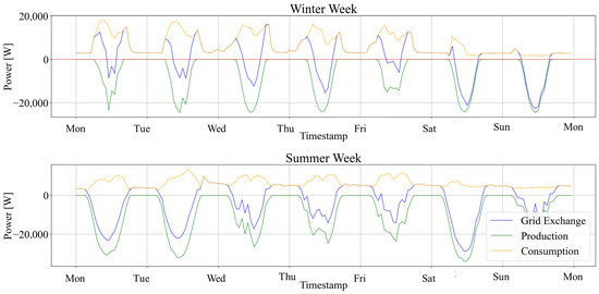
Figure 4.
Microgrid consumption and production behavior in a winter (above) and summer (below) week.
Historical data on EVs provided in this Case Study include information from September 2023 to June 2025, depending on the vehicle. The OBD device collected data about: instant velocity, odometer, charging state, timestamp, and battery SoC. To extend the variables used by the ML algorithms, the data were ordered and resampled, and these new features were calculated.
Distance traveled (expressed in km) was calculated as the difference between two consecutive odometer readings:
where and are the odometer readings at the initial and final timesteps, respectively. The odometer has a sensitivity of 0.1 km.
Energy consumption (in kWh) was calculated from the variation in the State of Charge (SoC), multiplied by the real battery capacity of each EV:
where is the nominal usable capacity of the battery (kWh), and , are the initial and final SoC values in percent.
Specific consumption (expressed in kWh/100 km) was computed as the ratio between energy consumption and distance traveled, multiplied by 100:
Average velocity (expressed in km/h) was calculated as the ratio between the traveled distance and the time interval between two timesteps:
where is the elapsed time, expressed in hours.
In this work, several assumptions were introduced to simplify implementation and reduce computational costs:
- The effective battery capacity was assumed to be 85% of the nominal value, as some vehicles had been in use for more than five years [39].
- The specific energy consumption was assumed to depend only on the change in SoC, and not on its absolute level.
- The charging efficiency () was considered constant and equal to 0.8.
- No power losses were considered between the charging stations, the building, and the grid exchange meter to simplify the models. This assumption is based on the relatively short distances between the different components, typically less than 50–100 m.
Before being analyzed for ML purposes, the data required several preprocessing steps to ensure correct integration into the DT. Different criteria were chosen to filter data and consider only relevant measurements. Precisely, these filters include:
- taking into consideration only velocities between 10 km/h and the speed limit of each vehicle;
- limiting the values of specific consumption to below 30 kWh/100 km;
- The traveled distance (d) had to exceed 0.01 m to ensure that the vehicle was in motion;
- Outliers were removed by excluding data points with a z-score greater than 3 for each vehicle dataset.
In this manner, entries for each vehicle were calculated, and a summary of these is presented in Table 2. Simulations and analysis were conducted using a notebook with 16 GB RAM, an i7-12750H, and an RTX 4060. For the EV data analysis, collecting and processing all entries from the .json files (approximately 7 million records) required 61 s. It should be noted that this analysis and filtering step may take some time; however, it is performed only when the vehicle consumption models are updated, which occurs once a month, as agreed upon with the user. As velocity was one parameter that could be known prior to the user and input before starting an optimization, a correlation between this and the consumption was calculated. Specifically, Table 1 reveals that these two quantities are lowly correlated, ranging from person correlation values of −0.01 to 0.70 for Vehicle #2 and Vehicle #15, respectively. For this reason, it was not convenient to assess the specific consumption by the velocity using a supervised ML algorithm. Moreover, vehicles 11 to 15 present only a few entries which is related to their recent availability. Accordingly, the subsequent optimization process was limited to Vehicles 1–10.
Table 2.
Summary table of EV data.
4. Results
4.1. Optimization Algorithm Outcomes
Given the complexity of the trade-off between finding an optimal solution and reducing computational time, various algorithms and libraries were compared to identify the optimal solution. The algorithms included in this analysis are GA, NSGA-II, CGO, IGWO, and GWO-WOA, as they are among the most used in the current state-of-the-art related to microgrid optimization [40,41,42,43]. To test these algorithms, four different days were selected (two for winter and two for summer) to evaluate their performance under varying conditions. Specifically, for each season, a cloudy day and a sunny day were chosen, as seasonal variations affect not only solar radiation and, consequently, PV production, but also the duration of daylight. However, to maintain consistent boundary conditions, user preferences were assumed to remain constant for each day. Specifically, for Vehicle #2, a distance of 150 km, an average speed of 60 km/h, and an initial SoC of 25% were assumed. For Vehicle #6, a typical mixed route was considered, with an average speed of 30 km/h, a distance of 70 km, and an initial SoC of 10%.
In all cases, similar boundary conditions were applied across different algorithms: a population size of 500 individuals per generation and 500 generations (epochs) to prevent limiting the solution search. As shown in Table 3, on winter days, all the algorithms yielded similar objective function values (about EUR 52), with the exception of CGO. In this case, the cost was higher by EUR 4 as it was suggested to charge Vehicle #2 also at 4:00 am when no PV production was available. Focusing on a sunny day, as the availability of solar radiation is lower than in summer, it was possible to charge only the two vehicles needed. The charging periods in all the configurations were aligned with PV production, achieving a perfect balance between production and charging power. On a cloudy day, only the minimum SoC was achieved due to reduced PV production. As shown in Table 3, in both cases, IGWO and GWO-WOA outperformed the other algorithms, achieving the optimal solution up to 0.12% of the time (when comparing GA with GWO-WOA) and requiring fewer generations to converge. On the winter day, however, all algorithms succeeded in finding feasible solutions, demonstrating that when export is limited, all the algorithms converge in fewer than 332 generations.
Table 3.
Optimization results on winter days.
During the summer, it was observed that exceeding 100% SoC was always avoided, except in two distinct cases. In Table 4, as can be seen, only IGWO and GWO-WOA converged on both days without violating any constraints. Focusing on the results for a typical sunny summer day, IGWO and GWO-WOA performed the best, consistently converging in less than 1 min. Conversely, CGO, which performed well in winter, struggled during summer, failing to find an optimal solution. It exceeded the self-consumption constraint tolerance after 500 generations, requiring over 200 s. A similar pattern was observed with GA, which also took 500 generations and slightly exceeded the self-consumption tolerance but achieved a lower objective function value (EUR 23.1) compared to CGO (EUR 34.6), as some of the energy was sold instead of being self-consumed. NSGA-II found an optimal solution that maximized self-consumption; however, it predicted a SoC exceeding 100% for Vehicle #10, returning an infeasible solution. As expected, under cloudy conditions, the behavior resembled that of winter days, with IGWO and GWO-WOA converging more rapidly and producing feasible solutions. In contrast, CGO violated two constraints, as two vehicles exceeded 100% SoC and failed to achieve self-consumption, resulting in non-convergence. NSGA-II achieved the same optimal result as GWO-WOA but took more time and required more generations. The GA implementation violated two constraints: one that should limit the occurrence of alternative charging/discharging, and another that slightly exceeded the self-consumption tolerance. However, in both seasons, the GWO–WOA algorithm achieved the best performance among all tested methods, resulting in the lowest daily electricity costs while fully meeting user requirements.
Table 4.
Optimization results on summer days.
Figure 5 serves as an illustrative example of the hourly results from a single operational day, showing scenarios with high (top) and low (bottom) PV generation. On these days, it was assumed that a user requirement was to charge Vehicle #4 to 50% by 14:00 and Vehicle #6 to 40% by 18:00. In Figure 5, the attainment of the target SoC is indicated by a colored marker. The graph illustrates how the vehicles are fully charged during periods of potential energy export, thereby optimizing self-consumption. In addition, the vehicles are often charged beyond the required SoC levels when sufficient PV generation is available. For instance, the final SoC of Vehicle #4 reaches 56% at 14:00, exceeding the user-specified target. When the available export capacity is insufficient to fully meet the EV charging requirements specified by the user, the algorithm proposes a strategy that sources at least a portion of the energy needed for charging EVs during periods of excess PV production. As shown in Figure 5, this occurs between 10:00 and 14:00 and 15:00 and 18:00. In such cases, only the minimum SoC requirement is fulfilled, as expected.
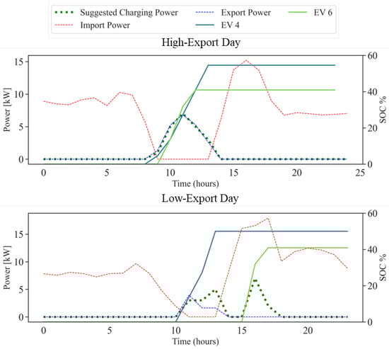
Figure 5.
Power trends and SoCs on winter days considering EV user preferences.
An 11-day test period was considered from 06/12/23 to 16/12/23, where the GWO-WOA algorithm was applied to historical data to assess its efficiency in saving energy for EV charging. During this period, which fell in winter, PV production was not always excessive, resulting in days when the algorithm recommended not charging the EVs. User preferences were excluded to simplify the testing process, as more than one day was considered simultaneously in the same simulation. During this period, PV generation peaked at 12.4 kW, with potential energy export occurring on 4 out of 7 days. As illustrated in Figure 6, the proposed algorithm employs charging strategies that utilize the available PV energy, both during high-export periods (the first 48 h of the week) and low-export periods (the last 48 h). These results confirm that the algorithm can effectively guide users in charging their EVs using self-generated power each day.
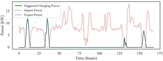
Figure 6.
Weekly Power trends for optimal EV charging compared to power import and export.
4.2. EV Consumption ML Models
To improve the reliability of EV consumption estimations, clustering techniques were applied to the available measurements for all vehicles. As previously mentioned, the Elbow method was employed to determine the appropriate number of clusters. As shown in Figure 7, the red marker, corresponding to a cluster number of four, lies at the elbow of the curve for each vehicle. Therefore, when applying K-Means clustering, four clusters were identified as the most appropriate choice for all 15 vehicles considered in the analysis. Selecting four clusters also provides a practical advantage, as it allows the DT to represent vehicle operation using only four average speed levels, thereby avoiding unnecessary complexity. For Vehicles #1 to #10, this choice resulted in WCSS values consistently ranging between 2000 and 100. For Vehicles #11 to #15, the scores were considerably lower due to the limited number of data points; however, in these cases, the Elbow criterion also supported the selection of four clusters.
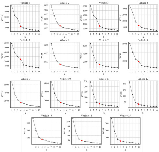
Figure 7.
Outcomes of elbow methods using K-Means on 15 vehicles (the red marker indicates the selected cluster number).
The clustering performance across 15 vehicles was evaluated using Calinski–Harabasz, Silhouette, and Davies–Bouldin indices (see Table 5). K-Means consistently delivered superior scores in most cases, particularly evident in the Calinski–Harabasz and Silhouette indices, indicating clear separation and internal cohesion among clusters. Gaussian Mixture Models (GMM) and Agglomerative clustering demonstrated variable performance, occasionally competitive but generally inferior to K-Means. Notably, vehicle 8 presented the highest Calinski score (11,585.3) with K-Means, while GMM underperformed with a Davies–Bouldin index of 1.345, suggesting increased overlap between clusters. Conversely, vehicles 11 to 15 exhibited lower Calinski scores, indicating inherently weaker clustering structures, likely due to the lower number of available entries. These findings suggest that K-Means is the preferred clustering approach for analyzing vehicle data; however, the algorithm choice may require adjustment based on specific vehicle characteristics.
Table 5.
Clustering performance across the 15 vehicles.
Finally, Figure 8 illustrates the position of the centroids and the clustering differentiation across all vehicles in the study. The analysis focuses on K-Means and agglomerative clustering, as these methods achieved the best performance (see Table 4). With a weight of 5 assigned to velocity, four centroids corresponding to different speed groups were identified. The results show that, depending on the vehicle and the number of available entries, similar patterns can be observed. For some vehicles (e.g., Vehicle #5 in Figure 8), consumption values at each centroid exhibit low variation across different speeds. Specifically, for Vehicle #5, consumption ranged between 12.5 and 20 kWh/100 km, with lower variability observed at higher speeds. In other cases, however, larger differences in consumption are observed between velocity ranges and their corresponding cluster centroids. For instance, in Vehicle #9, the centroid corresponding to the lowest speed (approximately 17 km/h) is associated with a consumption of 10.4 kWh/100 km, while at 57 km/h the consumption increases to 15.4 kWh/100 km. Comparing K-Means and agglomerative clustering, it is evident that agglomerative clustering produces less regular cluster boundaries, although the groupings remain similar to those obtained with K-Means. The consumption values associated with each centroid are also comparable between the two methods, with only minor differences observed. For instance, for Vehicle #9, the centroid of Cluster 3 corresponds to 39 km/h using K-Means and 47 km/h using agglomerative clustering. This difference arises because K-Means is more strongly influenced by variables with higher variance. As a result, in K-Means, points located near cluster boundaries show a sharper distinction between groups.
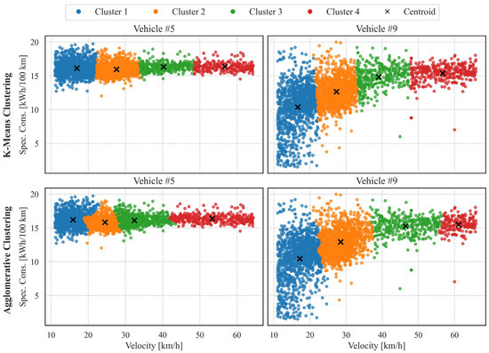
Figure 8.
Clusters and position of the centroids for K-Means and agglomerative clustering techniques.
Table 6 reports the K-Means clustering results for vehicle centroids. These values are integrated into the DT as user-defined speed inputs for customized optimization. For the process, from filtered data to the identification of centroids using the best clustering technique for all vehicles, the process required 46 s. Six out of fifteen vehicles show negligible sensitivity of consumption to velocity; for example, Vehicles #1–3 exhibit values between 16.0 and 16.5 kWh/100 km. In contrast, vehicles with larger variation display ranges from 7.3 to 15.8 kWh/100 km, with the highest deviations typically associated with limited datasets. In all cases, consumption increases with velocity, consistent with expectations. At low speeds, higher regenerative braking frequency contributes to improved efficiency. For vehicles with velocity-dependent consumption, centroid positions remain largely stable across clusters.
Table 6.
Centroid details for K-Means clustering for each vehicle.
4.3. Digital Twin Dashboard
The presented algorithms are finally implemented in the DT’s DSS, which focuses on optimizing EV charging processes to enhance self-consumption of generated power while also reducing costs. The implementation is based on APIs, following the architecture previously presented in [26] for DT. Within this DT, users can access real-time data from the homepage, such as the instantaneous power of each charging station plug, building energy consumption, and power output from the PV plant. Furthermore, as the EVs are fitted with OBD systems, continuous monitoring via the DT is available. This setup also allows for the constant refinement of vehicle consumption ML models through ongoing data collection. Finally, the collected data is utilized to train regressors, which are not the focus of this study, that forecast future PV production or building energy consumption, both of which can be viewed on the dashboard of the DT and serve as inputs for the optimization.
The DT implements three optimization strategies via the Middleware API, providing both day-ahead and real-time recommendations to facility managers on vehicle selection, charging schedules, and charging methods. The day-ahead optimization generates forecasts of plug power demand for the following day, together with State of Charge (SoC) projections. Through the DT dashboard, users define operational requirements by specifying which EVs will be needed the next day, the travel distance, and the expected itinerary type (based on velocity settings shown in Figure 9a). As shown, a button is located in the upper-left section of the dashboard, allowing the user to define or leave the charging start time undefined. This feature helps facility managers, even those without specific charging requirements, identify how to schedule charging to maximize self-consumption. Once the input is submitted, the optimization is executed, and the results are displayed in the dashboard (Figure 9b), enabling users to evaluate and select the most appropriate strategy among the three presented in the Methodology section. Once a strategy is selected, the DT could autonomously control the charging station through an API, after the user connects the corresponding EV, as recommended by the optimization algorithm. On the vehicles page, users can view the expected future EV SoC via a chart, which indicates the remaining charge hours.
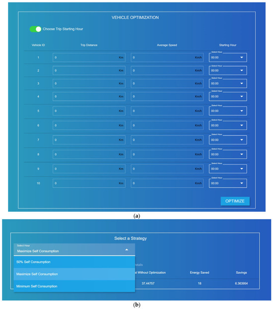
Figure 9.
Dashboard of the smart grid digital twin: vehicle selection page (a) and strategy selection page (b).
The real-time optimization algorithm can also adjust the power output of active plugs to better align on-site PV generation with building energy demand, thereby reducing both energy exports and imports from the grid (Figure 10). Once activated, the processor calculates a new charging power modulation for the charging stations, which is also displayed in a dedicated panel on the dashboard. In cases where modulation options are limited, for example, when only a single vehicle is connected, the DSS interface provides guidance by suggesting which vehicle to connect or recommending adjustments to the HP setpoint to modify building electricity consumption. An illustrative case is shown in Figure 10, where the DSS panel prompts the user to lower the reversible HP setpoint and modify plug charging power. This approach would enable pre-cooling of the building during the day, thereby reducing cooling demand in the evening.
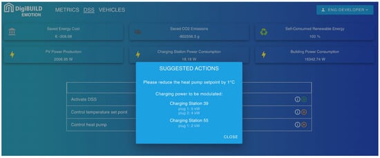
Figure 10.
Example of suggestions for the DSS of the smart grid.
5. Discussion
The developed DT demonstrated its capability to provide several useful outputs for the end user. The optimization based on the GWO–WOA algorithm, being a heuristic model, was able to identify local optima within a time frame suitable for real-time user interaction. The integration with the ML models for EV consumption was also tested and successfully supported charging recommendations. For the ML models, when a sufficient number of data entries were available (as for EVs #1–10), the clustering approach allowed each vehicle to be uniquely characterized. Among these, five vehicles showed an average variation in consumption of only 0.2 kWh/100 km across different velocity range centroids, while in some cases the variation reached up to 3 kWh/100 km.
Throughout the DigiBUILD project, continuous collaboration ensured active involvement of the end user in the development of the DT. It is evident, based on the findings of this study, that the implementation of this technology has yielded a variety of benefits. Firstly, a 25.7% reduction in energy drawn from the grid was achieved through the more efficient use of available EVs within the DT framework. This reduction corresponds to an annual reduction of approximately 4.2 tCO2 in GWP emissions [44]. Furthermore, self-consumption expectations were met, with the self-consumption rate increasing from 60% to 80%. Finally, by improving energy awareness through the DT, the company identified the need to install an additional charging station, moving closer to its net-zero targets.
To the best of the authors’ knowledge, compared to previous studies, this work represents the first implementation of a DT that integrates interactive user preferences, EV modeling, and charging optimization. The most comparable study is Ref. [15], which considered optimization under user preference constraints. However, this study did not include EV modeling (treating EVs only as shiftable loads) or implementing a DT framework. In terms of algorithm performance, the GWO–WOA algorithm in this study achieved an optimal charging solution in under 21 s on a cloudy winter’s day, significantly faster than the 197 s reported in Ref. [9] and 97 s in Ref. [11]. Nevertheless, metaheuristic algorithms can struggle to identify global optima, and mathematical solvers can yield faster charging schedules when the optimization problem is well formulated. For instance, Ref. [12] achieved optimal scheduling at hourly intervals over a one-week horizon in 35 s. The clustering-based method for estimating EV consumption also represented an improvement over using a fixed average consumption, as in Ref. [16]. This approach required only two input variables, whereas more accurately supervised learning models in Ref. [22] and Ref. [23] required 14 and 9 inputs, respectively, thus increasing computational complexity. Overall, comparing the proposed DT architecture with state-of-the-art methods confirms that it achieves satisfactory computational efficiency for real-time operation, relying on limited input data and moderate hardware resources.
The developed DT operated effectively under different meteorological conditions. The proposed methodology can be replicated in broader contexts, such as microgrids that integrate additional energy systems, including battery storage and small-scale wind generators. The DT architecture relies entirely on open-source tools, while the sensing layer incorporates various meters and OBD devices for vehicles. However, certain limitations are introduced by several assumptions that were made. Additional constraints would need to be incorporated for larger microgrids, accounting for factors such as the distance between charging stations, power losses, multi-user interactions, and conditions to mitigate battery degradation. Furthermore, the accuracy of the ML models could be improved, as it was limited in this study by the amount of available data. To enhance both optimization performance and model accuracy, future work should explore hybrid approaches combining electronic systems, data-driven techniques, and physics-based methods, as presented in [45].
Finally, to further improve the proposed methodology, several directions should be explored. New optimization constraints should include parameters related to EV battery degradation, in order to limit its impact during operation. With regard to EVs, it is important to note that additional parameters identified in previous studies, such as load ratio, maximum speed, latitude and longitude, and road slopes, should be collected through the existing OBD systems or provided directly by the user. From an optimization perspective, multi-objective approaches should be considered in order to account for system flexibility and integration with other components of the smart grid or with grid operators. In addition, the utilization of non-heuristic optimization methods should be explored to facilitate the identification of optimal solutions, rather than local optima. The DSS could also be enhanced by incorporating more advanced recommendations for heat pump management, including thermal comfort indicators (if indoor sensors are available) and potential inputs from energy community operators.
6. Conclusions
ML and optimization algorithms have been extensively studied in the recent literature for balancing the charging of EVs with available RESs. However, the majority of these contributions remain theoretical, with limited deployment in real-world case studies. This work partially addresses this gap by presenting a case study developed within the DigiBUILD European project. A DT was designed and implemented for a microgrid in Italy, integrating unsupervised learning models and optimization algorithms. The microgrid comprises 15 EVs, a building equipped with 50 kWp of PV, and two 22 kW EV charging stations (four plugs in total). The DT provides charging schedules based on user preferences, aiming to reduce energy costs by maximizing the use of on-site PV generation. Simulations conducted using historical data showed that the optimization algorithms provided solutions for maximizing EV self-consumption in under 25 s. In particular, IGWO-WOA and CGO consistently achieved optimal solutions in shorter times compared to other heuristic algorithms tested. Regarding the ML models, clustering analysis demonstrated that EV consumption could be effectively correlated with speed, with four clusters representing the majority of vehicles. Using K-Means, 9 out of 15 vehicles exhibited increasing consumption with increasing velocity. The models used were integrated into the DT through a middleware API. Finally, a user-oriented DSS was incorporated into the DT dashboard to provide actionable recommendations, such as connecting or disconnecting EVs based on grid conditions or adjusting HVAC setpoints. The real-time processor also enabled dynamic balancing of PV production and building demand by modulating charging power. Thanks to the DT, the facility manager was provided with an easy-to-use tool that enabled an increase in self-consumption of up to 80% during real testing. Future developments could incorporate more accurate methods for estimating EV consumption as additional vehicle data becomes available. Furthermore, the optimization framework could be extended with additional strategies and constraints, including multi-objective formulations, to better support grid operation. The deployment of such tools will be critical for achieving broader goals in energy efficiency and sustainability.
Author Contributions
Conceptualization, T.T. and M.B.; Methodology, T.T., F.B., D.A. and M.B.; Validation, T.T. and F.B.; Investigation, D.A. and M.B.; Data curation, T.T. and F.B.; Writing—original draft, T.T. and M.B.; Writing—review and editing, T.T., F.B., D.A. and M.B.; Visualization, T.T.; Supervision, D.A. and M.B. All authors have read and agreed to the published version of the manuscript.
Funding
This research was funded by the European Union’s Horizon Europe program under grant agreement No. 101069658 (DigiBUILD project).
Data Availability Statement
The original contributions presented in this study are included in this article; further inquiries can be directed to the corresponding author.
Acknowledgments
The authors would like to thank the DigiBUILD project consortium for the valuable collaboration and technical support provided during the development of this work. This research was conducted within the framework of the Horizon Europe program under grant agreement No. 101069658. The content of this paper reflects only the authors’ views, and the European Commission is not responsible for any use that may be made of the information it contains. All authors have read and agreed to the published version of the manuscript.
Conflicts of Interest
Author Francesco Bellesini was employed by Emotion S.r.l. in the Research and Development department. Author Diego Arnone was employed by Engineering Ingegneria Informatica S.p.A. in the Research and Innovation Department. The remaining authors declare that the research was conducted in the absence of any commercial or financial relationships that could be construed as a potential conflict of interest.
Abbreviations
The following abbreviations are used in this manuscript:
| API | Application Programming Interface |
| CGO | Chaos Game Optimization |
| DSS | Decision Support System |
| DT | Digital Twin |
| EU | European Union |
| EV | Electric Vehicle |
| GA | Genetic Algorithm |
| GHG | Greenhouse Gases |
| GMM | Gaussian Mixture Models |
| GWO-WOA | Grey Wolf Optimization—Whale Optimization Algorithm |
| HP | Heat Pump |
| HVAC | Heating, Ventilation, and Air Conditioning |
| IGWO | Improved Grey Wolf Optimization |
| K-Means | K-Means Clustering |
| LSTM | Long Short-Term Memory |
| ML | Machine Learning |
| NSGA-II | Non-dominated Sorting Genetic Algorithm II |
| OBD | On-Board Diagnostics |
| PV | Photovoltaic |
| RESs | Renewable Energy Sources |
| SoC | State of Charge |
| XGBoost | Extreme Gradient Boosting |
References
- International Energy Agency IEA World—Emissions. Available online: https://www.iea.org/world/emissions (accessed on 25 August 2025).
- European Alternative Fuels Observatory Italy—Incentives and Legislation. Available online: https://alternative-fuels-observatory.ec.europa.eu/transport-mode/road/italy/incentives-legislations (accessed on 25 August 2025).
- Kumar, P.; Channi, H.K.; Kumar, R.; Rajiv, A.; Kumari, B.; Singh, G.; Singh, S.; Dyab, I.F.; Lozanović, J. A Comprehensive Review of Vehicle-to-Grid Integration in Electric Vehicles: Powering the Future. Energy Convers. Manag. X 2025, 25, 100864. [Google Scholar] [CrossRef]
- do Amaral, J.V.S.; dos Santos, C.H.; Montevechi, J.A.B.; de Queiroz, A.R. Energy Digital Twin Applications: A Review. Renew. Sustain. Energy Rev. 2023, 188, 113891. [Google Scholar] [CrossRef]
- Sawhney, A.; Delfino, F.; Bonvini, B.; Bracco, S. EMS for Active and Reactive Power Management in a Polygeneration Microgrid Feeding a PED. Energies 2024, 17, 610. [Google Scholar] [CrossRef]
- Paixão, J.L.d.; Abaide, A.d.R.; Danielsson, G.H.; Sausen, J.P.; da Silva, L.N.F.; Neto, N.K. Optimized Strategy for Energy Management in an EV Fast Charging Microgrid Considering Storage Degradation. Energies 2025, 18, 1060. [Google Scholar] [CrossRef]
- Lin, F.J.; Lu, S.Y.; Hu, M.C.; Chen, Y.H. Stochastic Optimal Strategies and Management of Electric Vehicles and Microgrids. Energies 2024, 17, 3726. [Google Scholar] [CrossRef]
- Zacharopoulos, L.; Thonemann, N.; Dumeier, M.; Geldermann, J. Environmental Optimization of the Charge of Battery Electric Vehicles. Appl. Energy 2023, 329, 120259. [Google Scholar] [CrossRef]
- Bao, D.-W.; Zhou, J.-Y.; Zhang, Z.-Q.; Chen, Z.; Kang, D. Mixed Fleet Scheduling Method for Airport Ground Service Vehicles under the Trend of Electrification. J. Air Transp. Manag. 2023, 108, 102379. [Google Scholar] [CrossRef]
- Yin, W.; Ji, J.; Wen, T.; Zhang, C. Study on Orderly Charging Strategy of EV with Load Forecasting. Energy 2023, 278, 127818. [Google Scholar] [CrossRef]
- Ahmadi, B.; Shirazi, E. A Heuristic-Driven Charging Strategy of Electric Vehicle for Grids with High EV Penetration. Energies 2023, 16, 6959. [Google Scholar] [CrossRef]
- Fresia, M.; Robbiano, T.; Caliano, M.; Delfino, F.; Bracco, S. Optimal Operation of an Industrial Microgrid within a Renewable Energy Community: A Case Study of a Greentech Company. Energies 2024, 17, 3567. [Google Scholar] [CrossRef]
- Nguyen, T.L.; Nguyen, Q.A. A Multi-Objective PSO-GWO Approach for Smart Grid Reconfiguration with Renewable Energy and Electric Vehicles. Energies 2025, 18, 2020. [Google Scholar] [CrossRef]
- Mathur, D.; Kanwar, N.; Goyal, S.K. A Cost-Efficient Energy Management of EV Integrated Community Microgrid. In Flexible Electronics for Electric Vehicles; Springer: Berlin/Heidelberg, Germany, 2024; pp. 329–339. [Google Scholar]
- Uzair, M.; Ali Abbas Kazmi, S. A Multi-Criteria Decision Model to Support Sustainable Building Energy Management System with Intelligent Automation. Energy Build. 2023, 301, 113687. [Google Scholar] [CrossRef]
- Kaewdornhan, N.; Srithapon, C.; Liemthong, R.; Chatthaworn, R. Real-Time Multi-Home Energy Management with EV Charging Scheduling Using Multi-Agent Deep Reinforcement Learning Optimization. Energies 2023, 16, 2357. [Google Scholar] [CrossRef]
- Liu, J.; Wang, H.; Du, Y.; Lu, Y.; Wang, Z. Multi-Objective Optimal Peak Load Shaving Strategy Using Coordinated Scheduling of EVs and BESS with Adoption of MORBHPSO. J. Energy Storage 2023, 64, 107121. [Google Scholar] [CrossRef]
- Li, W.; Xu, X. A Hybrid Evolutionary and Machine Learning Approach for Smart Building: Sustainable Building Energy Management Design. Sustain. Energy Technol. Assess. 2024, 65, 103709. [Google Scholar] [CrossRef]
- Benedetto, G.; Bompard, E.; Mazza, A.; Pons, E.; Tosco, P.; Zampolli, M.; Jaboeuf, R. Integration of Electric Vehicles in Buildings: Optimization Model and Economic Assessment by a Digital Twin Representation. In Proceedings of the 2024 International Conference on Smart Energy Systems and Technologies: Driving the Advances for Future Electrification, SEST 2024—Proceedings, Torino, Italy, 10–12 September 2024; Institute of Electrical and Electronics Engineers Inc.: Piscataway, NJ, USA, 2024. [Google Scholar]
- Menyhart, J. Electric Vehicles and Energy Communities: Vehicle-to-Grid Opportunities and a Sustainable Future. Energies 2025, 18, 854. [Google Scholar] [CrossRef]
- Cavus, M.; Allahham, A. Spatio-Temporal Attention-Based Deep Learning for Smart Grid Demand Prediction. Electronics 2025, 14, 2514. [Google Scholar] [CrossRef]
- Zhao, L.; Yao, W.; Wang, Y.; Hu, J. Machine Learning-Based Method for Remaining Range Prediction of Electric Vehicles. IEEE Access 2020, 8, 212423–212441. [Google Scholar] [CrossRef]
- Yavasoglu, H.A.; Tetik, Y.E.; Gokce, K. Implementation of Machine Learning Based Real Time Range Estimation Method without Destination Knowledge for BEVs. Energy 2019, 172, 1179–1186. [Google Scholar] [CrossRef]
- Almeida, L.; Soares, A.; Moura, P. A Systematic Review of Optimization Approaches for the Integration of Electric Vehicles in Public Buildings. Energies 2023, 16, 5030. [Google Scholar] [CrossRef]
- DigiBUILD Project—High-Quality Data-Driven Services for a Digital Built Environment Towards a Climate-Neutral Building Stock. Available online: https://digibuild-project.eu/ (accessed on 27 June 2024).
- Testasecca, T.; Stamatopoulos, S.; Natalini, A.; Lazzaro, M.; Capizzi, C.M.; Sarmas, E.; Arnone, D. Implementing Digital Twins for Enhanced Energy Management in Three Case Studies. In Proceedings of the 2024 IEEE International Workshop on Metrology for Living Environment (MetroLivEnv), Chania, Greece, 12–14 June 2024; IEEE: Piscataway, NJ, USA, 2024; pp. 343–348. [Google Scholar]
- Ahmed, H.A.K.; Taqi, K.M.; Hassan, A.M.S.; Khaki, M. Joint Energy Management with Integration of Renewable Energy Sources Considering Energy and Reserve Minimization. Electr. Power Syst. Res. 2024, 232, 110412. [Google Scholar] [CrossRef]
- Yang, G.; Zhang, L.; Li, S.; Wu, X. Quantitative Energy Trading Strategies in Cooperative Microgrids in Electricity Market: A Multi-Dimensional Analysis of Risk and Return. Sol. Energy 2023, 262, 111860. [Google Scholar] [CrossRef]
- Shen, S.; Yuan, Y. The Economics of Renewable Energy Portfolio Management in Solar Based Microgrids: A Comparative Study of Smart Strategies in the Market. Sol. Energy 2023, 262, 111864. [Google Scholar] [CrossRef]
- Yang, H.; Zhang, S.; Zeng, J.; Tang, S.; Xiong, S. Future of Sustainable Renewable-Based Energy Systems in Smart City Industry: Interruptible Load Scheduling Perspective. Sol. Energy 2023, 263, 111866. [Google Scholar] [CrossRef]
- Blank, J.; Deb, K. Pymoo: Multi-Objective Optimization in Python. IEEE Access 2020, 8, 89497–89509. [Google Scholar] [CrossRef]
- Van Thieu, N.; Mirjalili, S. MEALPY: An Open-Source Library for Latest Meta-Heuristic Algorithms in Python. J. Syst. Archit. 2023, 139, 102871. [Google Scholar] [CrossRef]
- Gad, A.F. PyGAD: An Intuitive Genetic Algorithm Python Library. Multimed. Tools Appl. 2023, 83, 58029–58042. [Google Scholar] [CrossRef]
- Deb, K.; Pratap, A.; Agarwal, S.; Meyarivan, T. A Fast and Elitist Multiobjective Genetic Algorithm: NSGA-II. IEEE Trans. Evol. Comput. 2002, 6, 182–197. [Google Scholar] [CrossRef]
- Talatahari, S.; Azizi, M. Chaos Game Optimization: A Novel Metaheuristic Algorithm. Artif. Intell. Rev. 2021, 54, 917–1004. [Google Scholar] [CrossRef]
- Kaveh, A.; Zakian, P. Improved GWO Algorithm for Optimal Design of Truss Structures. Eng. Comput. 2018, 34, 685–707. [Google Scholar] [CrossRef]
- Obadina, O.O.; Thaha, M.A.; Althoefer, K.; Shaheed, M.H. Dynamic Characterization of a Master–Slave Robotic Manipulator Using a Hybrid Grey Wolf–Whale Optimization Algorithm. J. Vib. Control 2022, 28, 1992–2003. [Google Scholar] [CrossRef]
- Pedregosa, F.; Varoquaux, G.; Gramfort, A.; Michel, V.; Thirion, B.; Grisel, O.; Blondel, M.; Prettenhofer, P.; Weiss, R.; Dubourg, V.; et al. Scikit-Learn: Machine Learning in Python. J. Mach. Learn. Res. 2011, 12, 2825–2830. [Google Scholar]
- Yang, F.; Xie, Y.; Deng, Y.; Yuan, C. Predictive Modeling of Battery Degradation and Greenhouse Gas Emissions from U.S. State-Level Electric Vehicle Operation. Nat. Commun. 2018, 9, 2429. [Google Scholar] [CrossRef] [PubMed]
- Li, Q.; Cui, Z.; Cai, Y.; Su, Y. Multi-Objective Operation of Solar-Based Microgrids Incorporating Artificial Neural Network and Grey Wolf Optimizer in Digital Twin. Sol. Energy 2023, 262, 111873. [Google Scholar] [CrossRef]
- Testasecca, T.; Stamatopoulos, S.; Lazzaro, M.; Sarmas, E. Recent Advances on Data-Driven Services for Smart Energy Systems Optimization and pro-Active Management. In Proceedings of the 2023 IEEE International Workshop on Metrology for Living Environment (MetroLivEnv), Milano, Italy, 29–31 May 2023. [Google Scholar]
- Fan, X.; Li, Y. Energy Management of Renewable Based Power Grids Using Artificial Intelligence: Digital Twin of Renewables. Sol. Energy 2023, 262, 111867. [Google Scholar] [CrossRef]
- Xu, J.; Gong, J. Novel Sustainable Urban Management Framework Based on Solar Energy and Digital Twin. Sol. Energy 2023, 262, 111861. [Google Scholar] [CrossRef]
- Costa, N.; Serroni, S.; Cipollone, V.; Morresi, N.; Revel, G.M.; Meng, W.; Antoine, A.; Bogdan, O.; Celestino, P.M.; Vandi, L.; et al. Deliverable D5.5|Impact Analysis, Lessons Learnt and Replication Guidelines; DigiBUILD Project, funded by the European Union’s Horizon Europe programme under Grant Agreement No. 101069658; European Commission: Brussels, Belgium, 2025. [Google Scholar]
- Suvorov, A.; Gusev, A.; Ruban, N.; Andreev, M.; Askarov, A.; Ufa, R.; Razzhivin, I.; Kievets, A.; Bay, J. Potential Application of HRTSim for Comprehensive Simulation of Large-Scale Power Systems with Distributed Generation. Int. J. Emerg. Electr. Power Syst. 2019, 20, 20190075. [Google Scholar] [CrossRef]


Disclaimer/Publisher’s Note: The statements, opinions and data contained in all publications are solely those of the individual author(s) and contributor(s) and not of MDPI and/or the editor(s). MDPI and/or the editor(s) disclaim responsibility for any injury to people or property resulting from any ideas, methods, instructions or products referred to in the content. |
© 2025 by the authors. Licensee MDPI, Basel, Switzerland. This article is an open access article distributed under the terms and conditions of the Creative Commons Attribution (CC BY) license (https://creativecommons.org/licenses/by/4.0/).