Abstract
This contribution investigates whether the use of the MATLAB Optimization Toolbox on a parameter identification problem for a TRNSYS model provides better performance in iteration time. It presents the development of a framework connecting the MATLAB Optimization Toolbox with TRNSYS on the one hand and coordinating the optimization process of a TRNSYS model by GenOpt through MATLAB on the other hand. A benchmark framework in MATLAB was created to link TRNSYS and MATLAB and to configure the optimization process of GenOpt and the MATLAB Optimization Toolbox. Using this framework, a comprehensive comparison of the optimization solvers in GenOpt and the MATLAB Optimization Toolbox for the identification of the overall heat transfer coefficient of a TRNSYS heat exchanger model regarding the optimization time and number of iterations is presented as a use case. The results for the given problem show that GenOpt gives slightly better results in optimization time, whereas MATLAB has more potential and flexibility.
1. Introduction
Control of Building Energy Systems (BES), which are part of the Building Automation and Control System (BACS), and their model-based design is a complex task comprising different domains and has increasingly become established in the energy industry and research. Nevertheless, these systems can further be improved by optimal design and control to be more cost-effective and reliable.
To this end, a large number of Building Performance Simulaton Tools (BPSTs) have been developed in recent decades [1]. A comprehensive list of BPSTs is provided in [2]. One reason for the increasing use of BPSTs is not in the least the increased legal requirements for BES. The revised Energy Performance of Buildings Directive (EPBD) (EU/2024/1275) entered into force in all EU countries on May 2024. An entire set of rules is applied here, for which EN 15232-1 [3] is used in sub-module M10 (Building Automation and Controls), in which the building is assigned to one of four BACS efficiency classes [4]. The amended version introduces new requirements for nonresidential and residential buildings, which should help to accelerate the gradual renovation of the entire building stock. In Germany, the new Building Energy Act (GEG 2023) regulates how the country will heat predominantly with Renewable Energies (RE) in the future. The GEG 2023 aims to increase the share of Renewable Energies in buildings sustainably and efficiently. According to the new requirements, new buildings’ BES will only be installed if they generate at least 65% of the heat provided using RE.
BPSTs are used in research and increasingly also in industry. They have different levels of model detail and cover the entire life cycle of BES, from the design, construction and operation of buildings to the acceleration and improvement of the design and planning process, improvement of building efficiency, development or optimization of building controls and evaluation of the market potential of new concepts.
At present, there exist domain-independent software tools with advanced control modeling features but less building simulation model capability and vice versa. Hence, an advanced approach is to combine the different software tools and their modular concepts by runtime coupling to incorporate their domain-specific advantages as model libraries, optimization algorithms or aided controller design [5].
There is currently no common standard established by all software manufacturers for the coupling of domain-specific software tools, although there are promising approaches such as Functional Mock-up Interface (FMI), which has now been developed to version 3.0 [6,7,8]. For this reason, considerable effort is still required in some cases to be able to use the various advantages of BPSTs for an application.
From the perspective of developers and researchers, the lack of standardized model exchange formats in the development of simulation studies poses the challenge of developing them according to the problems themselves. When faced with a selection of options, the question often arises as to which approach is easy to implement and also offers the best performance. The results of this study are intended to provide assistance in this regard.
In this article, we focus on three BPSTs, TRNSYS (17.02.0005 (32-bit)), MATLAB (2017b (64-bit)) and GenOpt (3.1.1), where TRNSYS is the central software for the creation of system models from the point of view of this contribution.
TRNSYS (TRaNsient SYstem Simulation Program) [9] is one of the BPSTs that is well-known for its numerous validation studies and its ability to model buildings incorporated with other systems, such as Heating, Ventilation and Air Conditioning (HVAC) and renewable energy sources. Based on numerical routines, it solves partial differential equation systems for dynamic system simulation. It enables the balancing of transient processes in a time-step resolution between hours and minutes. It has a modular structure comprising modules like multizone buildings and electrical and thermal energy systems. A disadvantage of TRNSYS is that the user-friendly integration of complex control and optimal system sizing methods is missing.
MATLAB (MATrix LABoratory) is a simulation environment for programming and numerical calculations [10], with a high variety of toolboxes, e.g., Optimization Toolbox and Parallel Computing Toolbox.
Generic Optimization Program (GenOpt) [11] is a software tool that allows multidimensional optimization of an objective function computed by any simulation tool that reads its input from a text file and writes its output to a text file.
This article describes a framework that can be used to combine TRNSYS and MATLAB in order to utilize the strengths of both programs. The framework is then applied to a simple optimization problem to investigate whether MATLAB has advantages in terms of performance for solving the optimization problem in comparison to a solution, where TRNSYS is coupled with GenOpt.
This paper is organized as follows: Section 2 discusses the most common methods of software coupling to TRNSYS and previous work in a literature review to identify the research gap that this paper aims to close. Section 3 describes the benchmark model implementation in TRNSYS for the one-dimensional optimization problem and the framework of coordinated optimization by GenOpt through MATLAB, as well as using the MATLAB optimizer solely with TRNSYS. In Section 4, the chosen solver parameters are listed, and the performance results are shown and discussed. A summary of the main findings and an outlook on further work concludes the contribution in Section 5.
2. Related Work and Research Question
In this study, the focus was placed on TRNSYS as a commonly used BES modeling tool. This section is divided into two parts. Section 2.1 describes the technical interfaces of the tool coupling to TRNSYS according to the current state. Section 2.2 then describes application scenarios in a literature review in order to identify the research gap and pose the research question in Section 2.3.
2.1. Tool Coupling to TRNSYS
Several interfaces between simulation software tools have been developed or tested for tool coupling or co-simulation [12,13,14]. Coupling between different software tools can be implemented either in a strong or a loose way [15]. In strong coupling, the models of all the connected simulators iterate in each simulation time step until they converge. This shows higher accuracy at the cost of higher computational load. Contrary to this, in loose coupling, the exchange data are only transmitted at the beginning of each time step, and the feedback between the simulators lags by one simulation time step. In the following, some methods of tool coupling, especially between MATLAB and TRNSYS, are described.
2.1.1. Functional Mock-Up Interface (FMI)
FMI is an open standard software tool interface for exchanging simulation models. While exporting a model to a Functional Mock-up Unit (FMU) the resulting FMU file incorporates an XML description file and compiled C-code in a DLL file. FMU import in Simulink has been supported since version 2017b by an FMU import block. The importing and exporting of FMUs is available through an additional toolbox [16]. Within TRNSYS, only FMU export is available using an open-source adapter called Type 6139 [17].
2.1.2. Building Controls Virtual Test Bed (BCVTB)
Building Controls Virtual Test Bed (BCVTB) is an open-source framework for co-simulation and acts as middleware between several software tools, e.g., TRNSYS, MATLAB, Dymola and EnergyPlus as well as the FMI [18]. Data exchange between the tools is implemented through socket communication. In [13], a building controller was developed using co-simulation, where BCVTB connects MATLAB for controller design and EnergyPlus for building simulation. As a drawback, the authors identified the high simulation time. Furthermore, debugging of the co-simulation proved to be difficult, since BCVTB can only listen to ports.
2.1.3. TRNSYS Type 155
TRNSYS also has built-in support of external programs. In addition to Microsoft Excel, ANSYS Fluent, ESP-r, Java and more, it can also directly communicate with MATLAB via Type 155. This Type implements a connection to the MATLAB engine in a separate process through the Component Object Model (COM) concept. Type 155 can be used in two different calling modes, iterative mode (strong coupling) and real-time controller mode (loose coupling). A thermal use-case example to compare the computational efficiency and accuracy was published in [14]. The authors stated the system had higher flexibility to the user in comparison to BCVTB and FMI.
2.1.4. Open Platform Communications Unified Architecture (OPC UA)
Open Platform Communications Unified Architecture (OPC UA) is a platform-independent service-oriented architecture communication standard. It performs information interchangeability between the real controller and software tools. While MATLAB has a built-in OPC Toolbox, TRNSYS lacks this interface. In [19], Pan et al. give no details about the implementation.
2.1.5. TCP/IP
Using this communication protocol, tools are enabled to have a general interface. While MATLAB offers functions to create a Transmission Control Protocol/Internet Protocol (TCP/IP) client and server, TRNSYS does not, and the user has to create a custom type, as shown in [20].
2.1.6. Dynamic Link Library (DLL)
Another approach under Windows is either to compile TRNSYS types into a Dynamic Link Library (DLL) and call them in MATLAB or to compile MATLAB/Simulink models using a simulink coder (formerly real-time workshop) into a DLL and call it using TRNSYS [21,22].
2.1.7. TRNSYS Type 163/169
The TRNSYS standard Type 163 and Type 169 enable the transfer of TRNSYS simulation model states to Python. The two Python-calling types differ fundamentally from each other. Type 163 reads and writes files between TRNSYS and Python at each simulation step. Type 169, which is coded in C++, uses the C-API principle of Python as a direct communication interface. Although it embeds Python in the code, it requires extensive C wrapper code to enable direct communication between TRNSYS and Python.
2.1.8. TRNSYS Type 3157 (CFFI)
Compared to Type 169, the communication with the Python script has been significantly improved in Type 3157. This package calls a Python module at runtime, which is implemented in a Python file located in the same directory as the TRNSYS input file (the deck file). This script can use any package or library installed in the Python environment. Communication between the (Fortran) TRNSYS DLL and the Python environment takes place via a Foreign Function Interface, which is defined using the C Foreign Function Interface (CFFI) Python package [23].
2.1.9. File Input/Output (FIO)
The TRNSYS simulation engine can be directly executed via command prompt by typing the following:
- Path_to_TRNExe.exe\TRNExe.exe Path_to_Dck_file\Dck_file.dck \switch
where switch can be as follows:
- n: This skips the dialog boxes that inform the user at the end of simulation on errors during the simulation process and therefore enables a batch mode.
- h: This implies the n-switch and enables the hidden batch mode that makes TRNSYS completely invisible. Graphical output by online plotter is not possible and has to be disabled by setting parameter 9 of the online plotter to −1. As an advantage, the simulation will be speed up noticeably.
By modifying the deck file using text editors, model parameters can be changed automatically in order to carry out parameter studies. It can also be used to create entire models, as is possible with pytrnsys [24]. In this context, TRNSYS printer types can be added to the model, for example, to generate an output file that can in turn be used as an input in the optimization loops for optimization processes, which is the principle in GenOpt [11].
In this study, the File Input/Output (FIO) approach is also used to determine a model parameter in an optimization problem by means of error minimization. A TRNSYS–MATLAB framework was developed to enable the automated iteration process.
2.2. Review
There are several studies in the literature that have either examined the coupling of the various BPSTs or compared them with each other in terms of accuracy and runtime using a reference model.
Solmaz [25] provided a critical overview of the developments in the field of BPSTs in the study and evaluated the effectiveness of nine BPSTs in the design process. A group of validated and accurate BPSTs were examined, categorized and compared based on general characteristics, validation, interoperability, user adaptation, application/functions, strengths and limitations. The BPSTs were divided into two groups. The first group consists of planning tools such as Revit, Rhino and SketchUp and the second of detailed simulation tools such as EnergyPlus, DOE2 and TRNSYS. In addition, there is other software (OpenStudio, DesignBuilder, Green Building Studio) that uses the simulation programs of the other tools.
In their review, Barber and Krarti [26] examined the common optimization tools for the design and control of building energy systems and their combined use. They looked at multiobjective optimization problems and showed the typical flowcharts of the approaches used. The software tools were divided into three categories: simulation engines, graphical user interfaces and simulation environments. TRNSYS was assigned to the first category and MATLAB to the third. According to the authors’ classification, the main difference between simulation engines and environments is that the latter contain several plug-ins or features, while the former are essentially standalone programs.
Kalkan et al. [27] compared the simulation time for an absorption chiller and PVT collector model programmed in C++, MATLAB and Python and integrated into TRNSYS using Type 155 and Type 3157, respectively. Their results showed that the simulation speed decreases significantly from C++ to Python to MATLAB. The authors recommended the use of Python if MATLAB libraries do not have to be used explicitly.
Since TRNSYS is unable to estimate the effectiveness of evaporation during cooling, which is a typical passive design method, Nayak et al. [28] developed a MATLAB–TRNSYS integration in which TRNSYS was modified to model the simultaneous heat and moisture transport from the damp roof surface of a building. They used the building model (Type 56) and coupled MATLAB with TRNSYS using Type 155. The temperature of the underside of a damp roof calculated with MATLAB was used as the boundary temperature for the dummy roof in TRNSYS.
In their paper, Mazzeo et al. [29] compare three common simulation tools for building simulation, namely, EnergyPlus, IDA Indoor Climate and Energy (IDA ICE) and TRNSYS, with the experimental data of two solar test boxes equipped without and with a Phase Change Material (PCM) in the floor in three different warm, intermediate and cold periods. Measurements of the internal air temperature, the internal and external surface temperature of the glass and the internal surface temperature of the floor were used for this purpose. Their results showed that the three tools were very comparable in the absence of PCM. TRNSYS had the highest accuracy in the warm period, while this was the case for IDA ICE in the cold period. Overall, IDA ICE was the best tool in all periods. In the presence of PCM, it can be seen that IDA ICE achieved almost the same accuracy as was achieved without PCM, while the other tools delivered lower accuracies.
Magni et al. [30] described the modeling approaches of eight widely used BPSTs in their work and compared them on a monthly and hourly basis for the climate zones of Stockholm, Stuttgart and Rome using simulation results for the same office cell defined by International Energy Agency Solar Heating and Cooling (IEA SHC) Task 56. The results of the cross-comparison show that overall, a good match was achieved between all dynamic simulation tools. The simulation with EnergyPlus was the fastest, followed by TRNSYS and ALMABuild. The authors also emphasized that it took several iterations and great effort on the part of the modelers to achieve a good match between all tools.
Some research has been conducted by applying the free, available software tool GenOpt in order to automate TRNSYS runs and to minimize a cost function also supporting parallel computing optimization. However, GenOpt is not capable of handling multiobjective optimization. When associated with TRNSYS, GenOpt can automatically generate building (.bui) and deck (.dck) files, run TRNSYS with those files, save results and restart.
Asadi et al. [31] used a simulation-based multicriteria optimization method in their work. In their framework, they developed a combination of TRNSYS, GenOpt and a Tchebycheff optimization technique developed in MATLAB. The objective was to optimize the refurbishment costs, energy savings and thermal comfort of a residential building in order to choose the best retrofit strategy for a building (, see Table 1).
Magnier et al. [32] used a simulation-based Artificial Neural Network (ANN) to characterize building behavior and then combined this ANN with the multicriteria Genetic Algorithm NSGA-II (Nondominated Sorting Genetic Algorithm 2) for optimization. This methodology was used in the studies to optimize thermal comfort and energy consumption in a residential building (). The combination of the two algorithms was called the GAINN methodology. The simulation model was integrated into TRNSYS. The multiobjective optimization was carried out in two steps. In the first step, a database was automatically generated by varying the model parameters with the help of GenOpt, which was used for automated parameterization of the model. An ANN was trained on this, and the model parameters were optimized using NSGA-II in the second step.
Fernandes et al. [33] presented in their work the methodology and results of a simulation-based optimization and evaluation study of an adsorption storage system in combination with a solar collector system, which was carried out in TRNSYS and MATLAB. The absorption storage components were modeled in MATLAB and integrated into the TRNSYS model that included a hot water storage tank. Parameter optimization was performed with GenOpt, which can be coupled with TRNSYS to perform automated parameter variation. The Generalized Pattern Search (GPS) algorithm was used. Twelve parameters were varied with the aim of minimizing the additional heating requirement ().
Narayan et al. [34] developed a coupled simulation framework for the nonlinear, time-varying, deterministic, discrete-time power system problem using TRNSYS and MATLAB. Using this framework, a Model Predictive Controller (MPC) with a moving horizon of 24 h was developed for an integrated thermal and electrical system with multiple energy sources in a household optimized for self-consumption. The optimization was carried out using 3 different algorithms: Particle Swarm Optimization (PSO), Genetic Algorithms (GA) and GPS. The objective function formulates the increase in the noncontrollable renewable energy on the one hand and a reduction in the use of a gas boiler on the other hand.
A few publications have used the pytrnsys package [24] to automate simulation studies. The aim of the research work by Mylonas et al. [35] is to demonstrate the reliability, robustness and computational efficiency of a cloud-based application of an MPC called Smart Energy Management for an apartment building. This energy management framework was tested on a virtual building model in TRNSYS running via the pytrnsys package using an open-source distributed-event streaming platform for data exchange and synchronization. In their work, four different objective function were defined: maximizing self-consumption of on-site PV energy (), minimizing CO2 emissions (), minimizing electricity costs () and minimizing electric consumption of the heat pump ().
In the work of Arenas-Larrañaga et al. [36], a parametric analysis was carried out using pytrnsys and TRNSYS, taking into account 14 European climate zones, two heat pumps with different natural refrigerants (CO2 and propane), four solar collector areas and three ice storage volumes. The analysis is based on TRNSYS simulations using previously calibrated and validated models. The open-source package pytrnsys was used to set up the system visually and to automate the 700 simulations carried out and the postprocessing of the data. In order to analyze the energetic performance of proposed system, the Seasonal Performance Factor (SPF) as objective function () was used as evaluation indicator.
Meiers et al. [37] proposed a hardware-in-the-loop simulation architecture where they described a communication procedure between TRNSYS, BCVTB and MATLAB as the simulation part and LabVIEW (Laboratory Virtual Instrumentation Engineering Workbench) [38] as the communication node for the hardware of the real system using the Message Queuing Telemetry Transport protocol. BCVTB serves as middleware for the communication between TRNSYS and MATLAB, while MATLAB controls the simulation framework itself and ensures the communication to LabVIEW.
The literature research shows that there is a need for solutions for coupling different BPSTs, especially with TRNSYS. A distinction can be made between problems relating to the control of BES, the design of such and the integration of tool-specific models into larger-scale models. First, both mentioned sub-areas mainly result in the solution of an optimization problem for which high-performance solution algorithms are required, especially if there are nonlinear relationships within the systems. To the authors’ knowledge, no study to date has shown a more comprehensive comparative study of solvers from GenOpt and the MATLAB Optimization Toolbox for a single-objective optimization problem, including a more detailed description of the tool coupling between MATLAB and TRNSYS. Narayan et al. described their framework using a DOS command and the processing of the deck file using MATLAB without going into more detail. Mylonas et al. and Arenas-Larrañaga et al. used the Python-based pytrnsys, whereas MATLAB is considered here. The cited publications consider a maximum of three solvers (Narayan et al.), while in this paper, six solvers of GenOpt and nine solvers of the MATLAB Optimization Toolbox are compared.
2.3. Research Question
The analysis of the reviewed literature shows that there is a research gap with regard to a comprehensive comparison of algorithms for optimizing a TRNSYS model under the aspect of system design (cf. Table 1). This is the starting point for the analysis presented in this contribution. Only the software tools TRNSYS, MATLAB and GenOpt as the solver engine or the MATLAB Optimization Toolbox, respectively, were considered here.
Therefore, the main research question is as follows:
Is there an advantage to using GenOpt via direct connection to TRNSYS compared to using the algorithms of the MATLAB Optimization Toolbox via the specially developed TRNSYS–MATLAB framework in terms of computation time and accuracy of the solution?
In this study, the focus is on model parameter identification by means of an error minimization process using a TRNSYS model. For this purpose, a simple example of a heat exchanger is used to determine the heat transfer coefficient.

Table 1.
Review comparison.
Table 1.
Review comparison.
| Publication | Purpose of Tool Coupling | Tool Coupling Method with TRNSYS | Used Software Tools and Programming Languages | Used Metrics | ||||||||
|---|---|---|---|---|---|---|---|---|---|---|---|---|
|
Optimization Objectives | Automation | Model Extension | Parametric Analysis | Model Comparison | ||||||||
| Design-Oriented | Operation-Oriented | Number and Name of Solvers | ||||||||||
| Single | Multi | |||||||||||
| Kalkan et al. [27] | - | - | - | - | - | - | xC,P,M | - | - | Type 155M Type 3157P DLLC | TRNSYS MATLAB C++ | |
| Nayak et al. [28] | - | - | - | - | - | - | xM | - | - | Type 155M | TRNSYS MATLAB | MAE |
| Mazzeo et al. [29] | - | - | - | - | - | - | - | - | x | - | TRNSYS EnergyPlus IDA ICE | RMSE, , NRMSE |
| Magni et al. [30] | - | - | - | - | - | - | - | - | x | - | TRNSYS EnergyPlus IDA ICE Simulink CarnotUIBK ALMABuild Modelica DALEC PHPP | RMSE, , MAE, MBE |
| Asadi et al. [31] | x | - | - | xM | 1 (bintprog)M | xG | - | - | - | FIOG,M | TRNSYS MATLAB GenOpt | |
| Magnier et al. [32] | x | - | - | xM | 2 (ANN NSGA-II)M | xG | - | - | - | FIOG | TRNSYS MATLAB GenOpt | |
| Fernandes et al. [33] | x | - | xG | - | 1 (GPS CS)G | - | xM | - | - | n/a | TRNSYS MATLAB GenOpt | |
| Narayan et al. [34] | - | x | - | xM | 3 (PSO, GA, GPS)M | - | - | - | - | FIOM | TRNSYS MATLAB | |
| Mylonas et al. [35] | - | x | xO | n/a | xpt | xP | - | - | Type 1630ct | TRNSYS Python pytrnsys OR tools | ||
| Arenas-Larrañaga et al. [36] | - | - | - | - | - | xpt | - | x | - | FIOpt | TRNSYS pytrnsys | |
| Meiers et al. [37] | - | - | - | - | - | xM | xM | - | - | BCVTB | TRNSYS MATLAB BCVTB LabVIEW | RMSE |
| Tadayon et al. [39] | x | - | xG | xM | 2 (MOPSO NSGA-II)M | xM | xM | - | - | FIOG,M | TRNSYS MATLAB GenOpt | |
| This paper | x | - | xM,G | - | 6 *,G,9 *,M | - | - | - | - | FIOG,M | TRNSYS MATLAB GenOpt | , AE |
M: MATLAB. G: GenOpt. pt: pytransys. P: Python. O: OR tools. C: C++. n/a: not available. FIO: File Input/Output. *: see Section 4. ct: custom TRNSYS type of Type 163 (Python). MAE: Mean Absolute Error. : Computation time. : coefficient of determination. RMSE: Root Mean Square Error. NRMSE: Normalized Root Mean Square Error. MBE: Mean Bias Error. : Objective Functions (see Section 2.2). AE: Absolute Error.
The framework for two approaches was developed and the results compared, where both of them are coordinated and automated by MATLAB:
- TRNSYS–GenOpt (TG).
- TRNSYS–MATLAB Optimization Toolbox (TM).
The objective of this study is to address the issues mentioned above in the following key aspects:
- Description of the design of both MATLAB–TRNSYS frameworks, TG and TM, respectively, for automated parameterization of models for design optimization and a parameter estimation as a use case.
- Comparison of the required computation times for the estimation process.
- Comparison of the solver accuracy for the estimation process.
In the following, this contribution focuses on calling TRNSYS model simulation runs via a command shell in the FIO approach through MATLAB.
An application of the framework described in Section 3 to a multiobjective optimization problem of BES was already described by Tadayon et al. [39]. The authors minimized a weighted sum of two single objectives (), which are the mean CO2 emissions and the average electricity costs.
The studies conducted here are limited to a single-objective optimization problem, which is, however, subjected to a more comprehensive comparison of the solvers.
3. Methodology
In this section, a short introduction to the used software tools is given. This is followed by the description of the TRNSYS benchmark model for tool coupling and the two frameworks, MATLAB-coordinated optimization of a TRNSYS model with GenOpt on the one hand and optimization with the MATLAB Optimization Toolbox on the other hand.
3.1. Introduction to the Used Software Tools
MATLAB is a high-level general-purpose modeling language. With its variety of extensions, called toolboxes, it is widely used in industry and research in the fields of control design, signal and image processing, optimization, communication and simulation [10]. The MATLAB Optimization Toolbox provides a set of algorithms that solve optimization problems. The toolbox includes functions for solving linear, quadratic, mixed-integer linear, nonlinear programming and least squares problems. TRNSYS is one of the most used simulation software programs for building and HVAC (Heating, Ventilation and Air Conditioning) system simulations. It has been commercially available since 1976 and uses a component-based modeling approach. By its modular structure, the software obtains flexibility. TRNSYS component models, also known as “Types”, can model complex multizone buildings, HVAC systems and renewable energy systems. For building dynamics, it is accepted as one of the most compressive and detailed simulation software programs [9]. GenOpt is an open-source optimization software program that evaluates a cost function by an external simulation program. Supported software tools are, for example, TRNSYS, Dymola and EnergyPlus. Its integrated libraries can solve one- and multidimensional problems with local and global solutions. If supported by the hardware, GenOpt automatically uses parallel computation. There are two modes in which GenOpt can be called, either in normal mode with a graphical user interface (GUI) or without GUI as a background process. For the following investigations, TRNSYS version 17.02.0005 (32-bit) with GenOpt 3.1.1 and MATLAB 2017b (64-bit) were used.
3.2. TRNSYS Benchmark Model
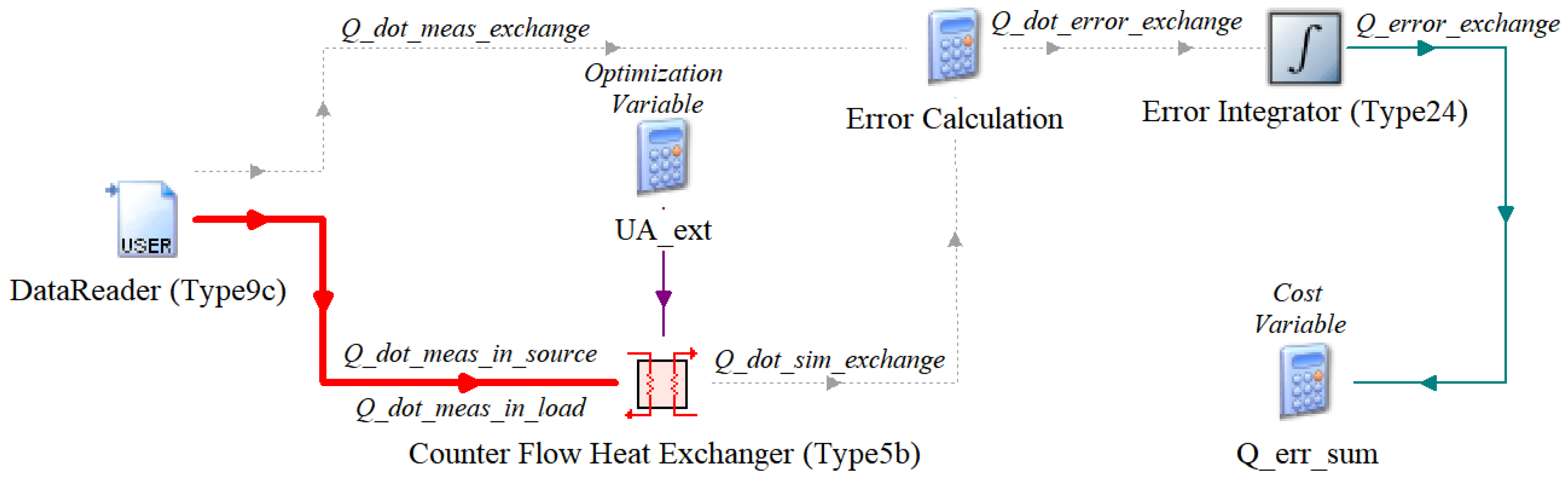
The TRNSYS benchmark model consists of a counterflow heat exchanger (Type 5b) that obtains measured time series data as input by a data reader (Type 9c), some error calculations and an error time integrator (Type 24). In Figure 1, the complete TRNSYS model is shown. The heat exchanger model measured fluid temperature and mass flow rate on the source and load side as input.

Figure 1.
TRNSYS benchmark model of a heat exchanger.
The heat exchange rate in kJ/(hK) is the optimization variable. The error between the measured heat exchange rate, , and the simulated one, , is calculated according to Equation (1).
Using the time integrator block, the complete sum of heat exchange error in kJ is calculated and used as the cost function for the optimization, using
3.3. Optimization Frameworks
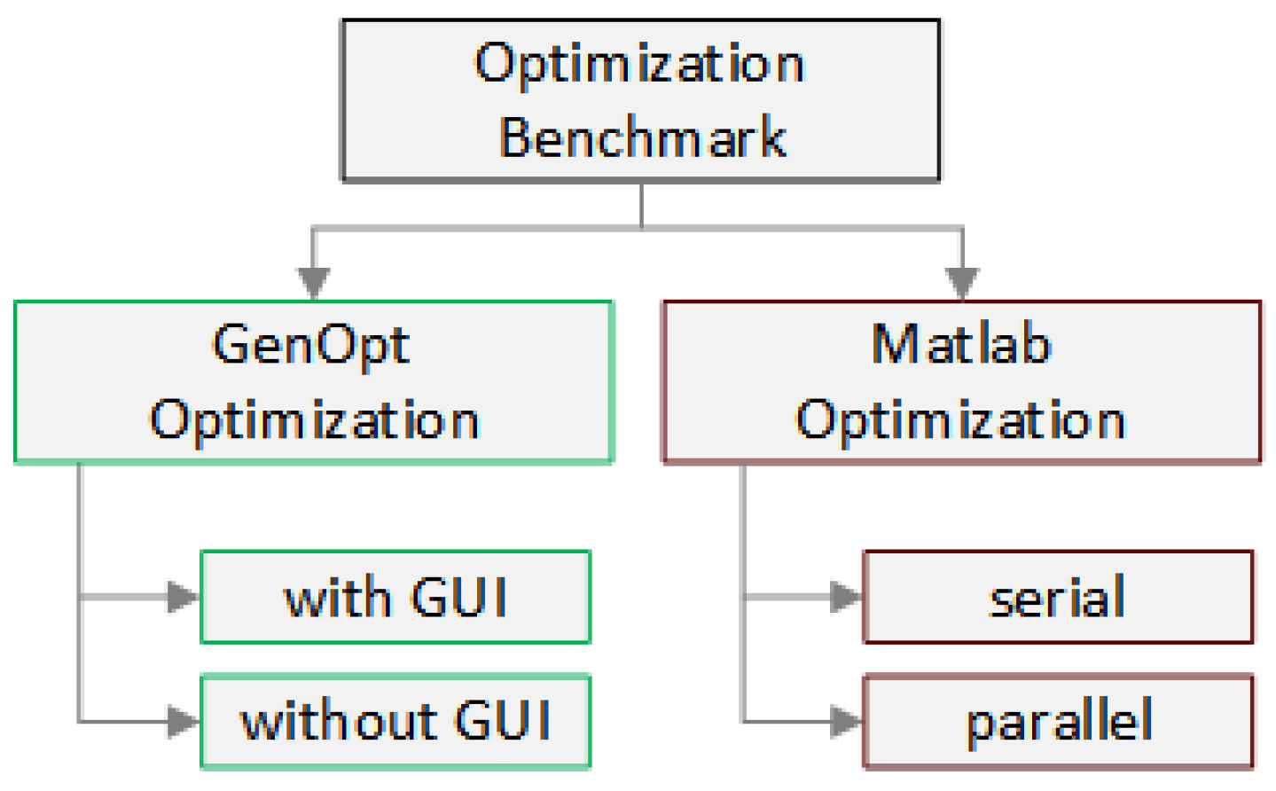
In the following, the two frameworks, a MATLAB-coordinated optimization of a TRNSYS model with GenOpt and an optimization with the MATLAB Optimization Toolbox, are described. As shown in Figure 2, there are four considered optimizer modes: in the GenOpt framework the standard way with a Grapical User Interface (GUI) or with suppressed GUI, and in the MATLAB optimization framework, solvers running in serial mode or in parallel simulation mode were taken into consideration.
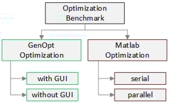
Figure 2.
Considered optimizer modes.
- A
- Coordinated coupling of TRNSYS and GenOpt by MATLABWithin the first framework, optimization is performed through GenOpt. In general, the complete process can be divided in three sections:
- 1
- Coordination.
- 2
- Optimization.
- 3
- Simulation.
By default, GenOpt has no functionality to start several solvers one after another automatically. To circumvent this disadvantage, MATLAB takes this over. In the coordination part, MATLAB calls GenOpt in different solver configurations in a loop. In the first section, MATLAB coordinates the user-defined configuration of the GenOpt files, such as file locations, algorithm choice and algorithm parameters, simulation configuration and its input. In general, when the user finishes the configuration in the GUI, GenOpt prepares the TRNSYS model deck file, which has to be created once in TRNSYS before starting the optimization process, to be a template as follows:- It replaces the optimization variable through the variable name in the case of a one-dimensional optimization problem.
- It adds an output printer, named Type 758, to write the chosen optimization variable value and the resulting cost variable value to the output files OutputListingMain.txt and OutputListingAll.txt. Note that in TRNSYS 18, the structure of the deck file changes at the end of the file, which makes further modifications necessary.
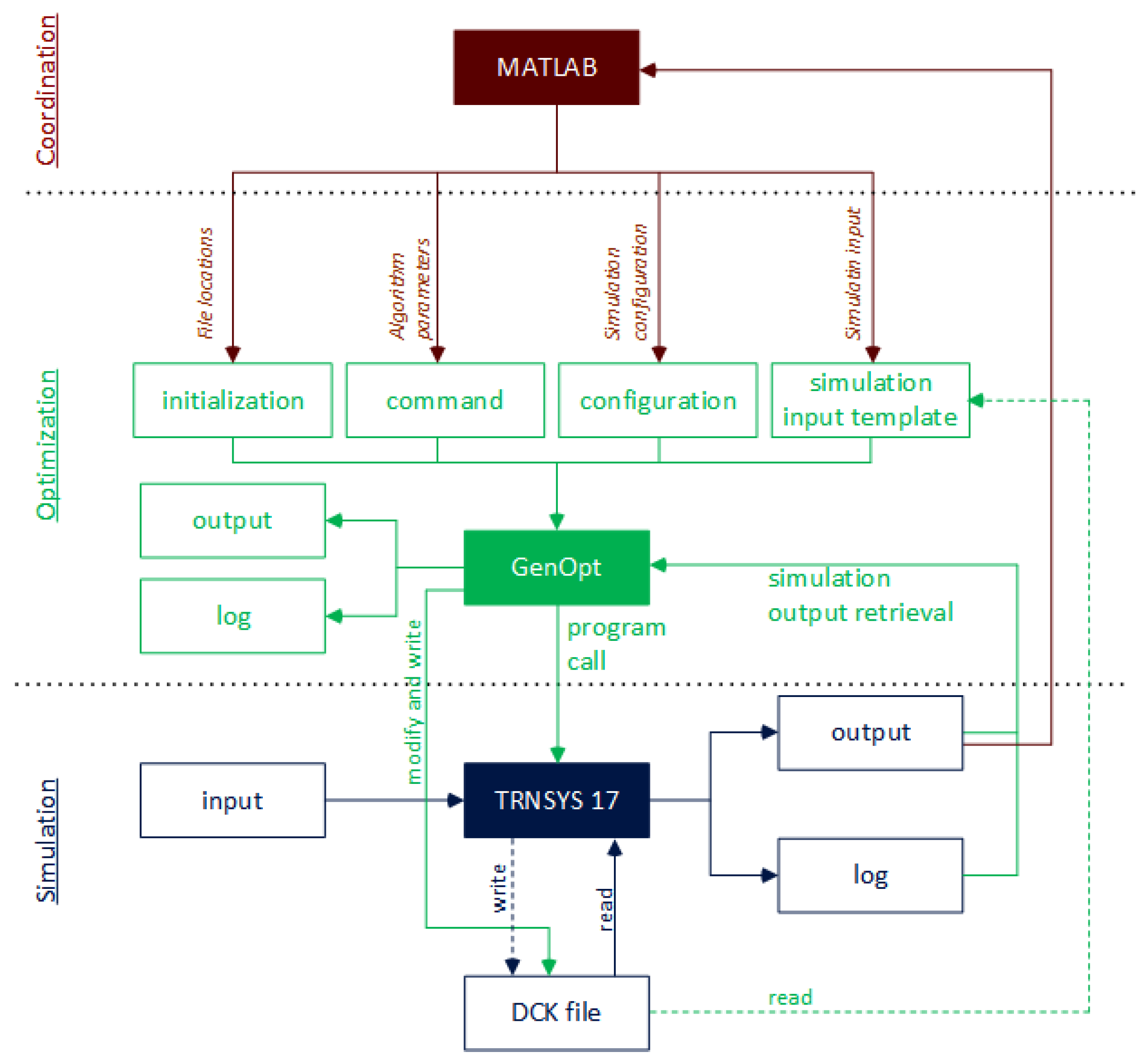
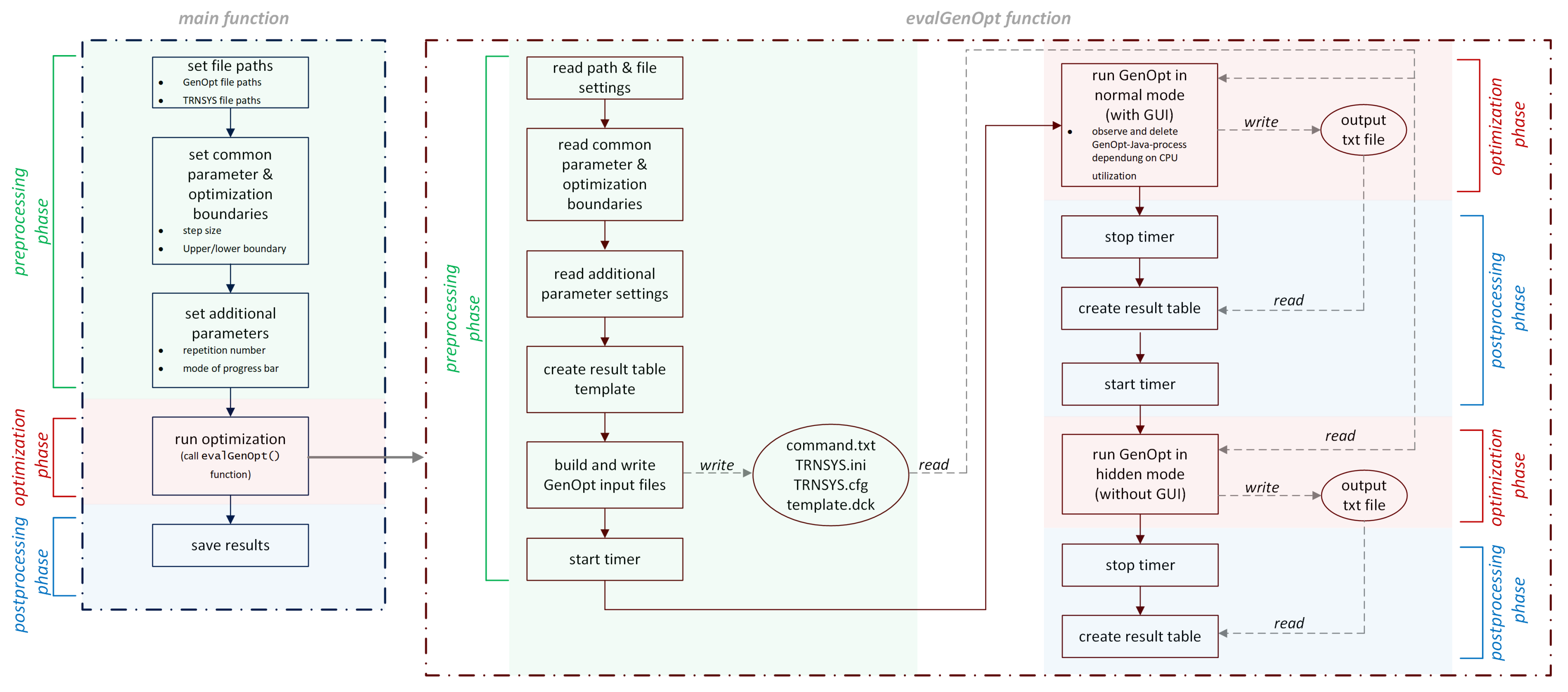
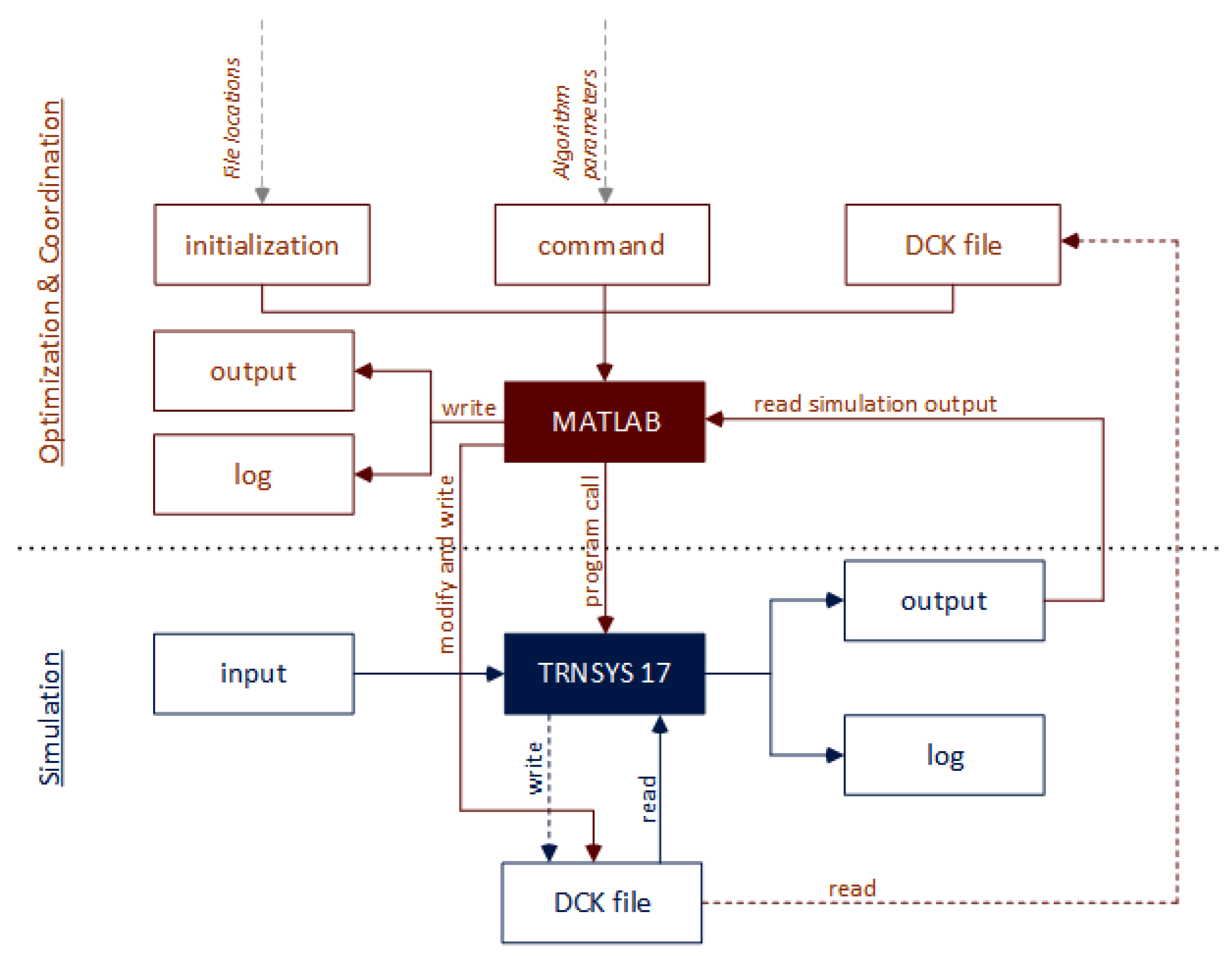
These two steps are also performed in the coordination part of the developed framework in MATLAB to bypass the configuration in the GenOpt GUI. The second section, optimization, is then handled mainly by GenOpt. For each optimization step, GenOpt writes a modified deck file and TRNSYS reads this modified template dck file and simulates the model (Section 3: simulation).Finally, MATLAB processes the output files of GenOpt for analysis and visualization of the results. Figure 3 shows the schema of the GenOpt interface [11] with the above described extensions.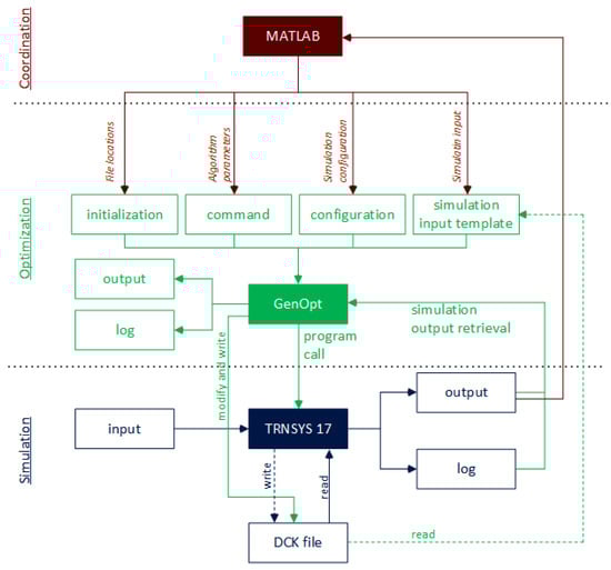 Figure 3. Tool coupling of MATLAB and GenOpt–TRNSYS [39] (based on [11]).In the following, the process flow of the coordination, optimization and simulation parts is called generic optimization and will be explained in steps that are more detailed. The generic optimization process has a main function and the evalGenOpt function. Both are subdivided into 3 phases (Figure 4):
 Figure 4. Flow chart of coordinated optimization through GenOpt by MATLAB.
- 1
- Preprocessing phase.
- 2
- Optimization phase.
- 3
- Postprocessing phase.
In the preprocessing phase of the main function, configuration steps are performed as listed below:- A table of all solver names is created.
- Paths are defined for the model deck file, GenOpt working directory in the TRNSYS path and new folder of the result files.
- Common solver parameters and boundary settings are defined, such as solver step size, min and max boundary values, initial start value, maximum iteration number and maximum number of equal results before optimization process stops.
- Additional parameter settings are defined, like the name of the optimization and cost variables, the number of repetitions of a complete optimization cycle to calculate a mean optimization time, mode of the TRNSYS simulation process bar during the optimization process and the number of time steps in idle state of the GenOpt GUI. The GenOpt GUI has no capability to close automatically when an optimization process has finished. Therefore, the process will be observed and terminated when it comes back to idle mode with no processor load for a user-defined time period as described later.
In the optimization phase of the main function, the GenOpt optimization with the user-defined parameters can be called as a MATLAB function:[output] = evalGenOpt(input)
where input are the configurations performed in the preprocessing part and the solver algorithm name of GenOpt. The output is a MATLAB data structure containing the optimization time, solution value, number of solver evaluations and objective value. In the postprocessing part, the result files are accumulated and processed for visualization. Within the evalGenOpt, function preprocessing is composed of extracting the date from the function input structure and writing the configuration files TRNSYS17.ini, TRNSYS.cfg, command.txt and template.dck. Then, sequentially, the optimization phase will be started once with GenOpt in normal mode with GUI using MATLAB’s system() command with the following input string:cmd /C java -jar genopt.jar TRNSYS.ini &
cmd starts a new instance of the Microsoft Windows command interpreter. /C carries out the command specified by the string and then terminates. The trailing & dispatches the command window to the background, while MATLAB can continue. This is required due to the drawback that the GenOpt GUI will not close itself or be closed by command attribute after the optimization has finished. Therefore, observation and manual termination of the task is implemented with the following .NET methods:System.Diagnostics.Process.GetProcessesByName(process_name)}, System.Diagnostics.PerformanceCounter(process_name)}.where java.exe is the GenOpt process name.Both GenOpt and the command window will be terminated when the CPU utilization is zero for a certain time (here 10 s) using the following in the MATLAB system() function:“C:\Windows\System32\taskkill.exe” /F /im java.exe /im cmd.exe
where /F forces the termination of the task specified with the parameter /im for the image or executable names. In hidden mode, without GUI, GenOpt can be started with the following command:java -classpath genopt.jar genopt.GenOpt TRNSYS.ini
After each of these two optimization phases, a timer is started to measure the optimization time for the benchmark, the GenOpt result txt file is read and data are collected. - B
- Coupling of TRNSYS and MATLAB Optimization ToolboxIn the second framework, the complete process can also be divided into the three sections coordination, optimization and simulation. In contrast to the first approach, the coordination and optimization are handled by MATLAB and its Optimization Toolbox, which triggers the simulation in TRNSYS. This approach is similar to that of GenOpt. MATLAB creates a copy of the dck files and modifies the optimization variable to fulfill the objective function. This takes into account the user configuration information of file paths and solver algorithm parameters. A TRNSYS output printer (Type 25) is added to the dck file, printing the objective value after each optimization iteration. MATLAB reads the objective value from this TRNSYS output file.When the solver finishes, the results of the optimization iteration process are written to a log file and an output file (Figure 5).
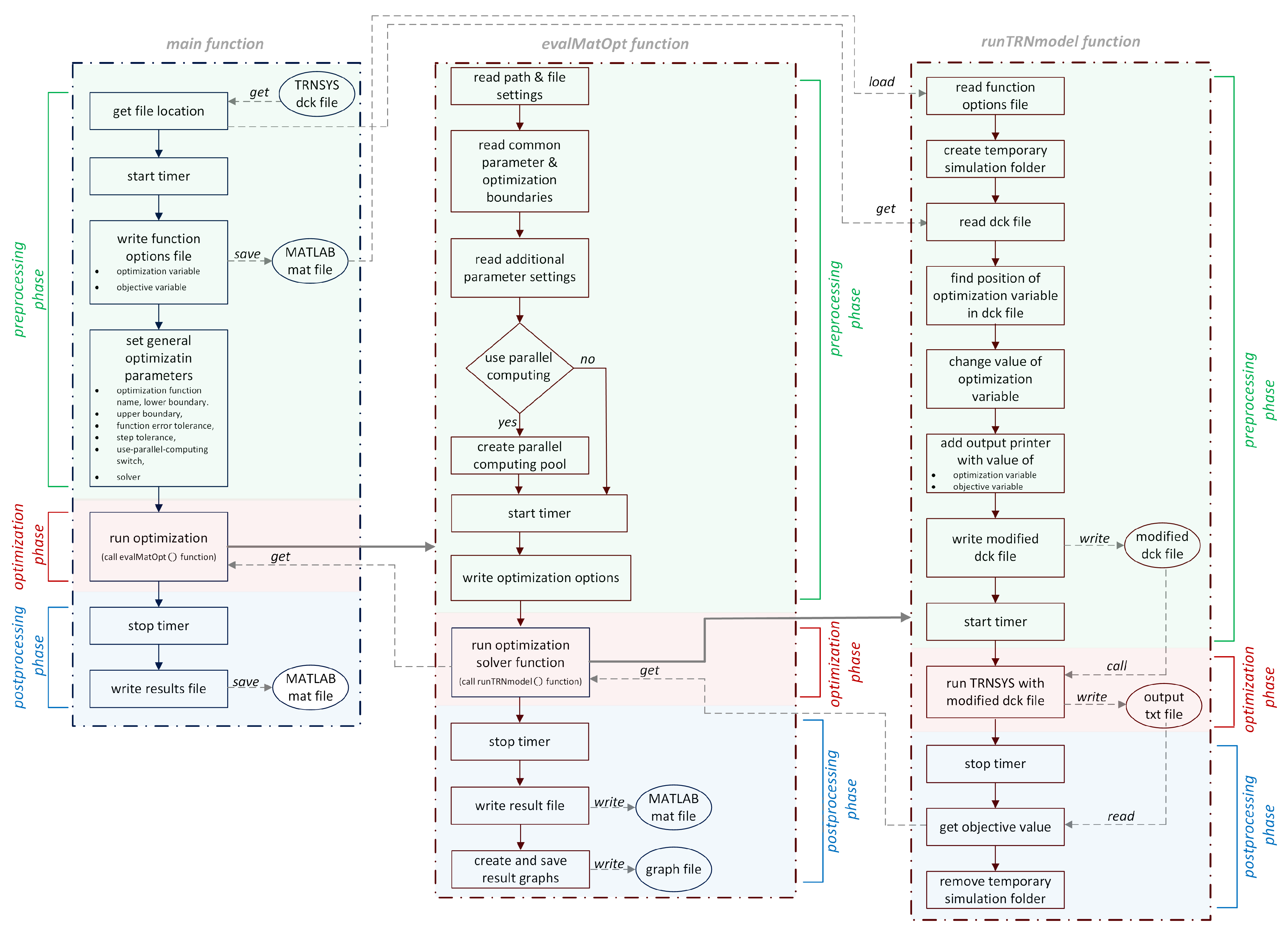
 Figure 5. Tool coupling of MATLAB and TRNSYS [39].The complete framework contains three function layers: main(), evalMatOpt() and runTRNmodel(). Each of the function layers can also be subdivided into a preprocessing, an optimization and a postprocessing phase (Figure 6).
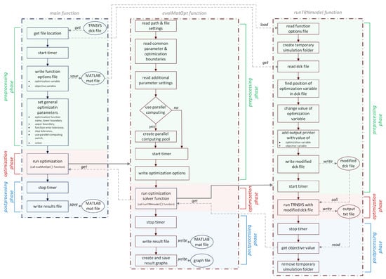 Figure 6. Flow chart of optimization by MATLAB.In the preprocessing phase of the main function, starting an optional timer to measure the overall processing time (not used for this benchmark) and declaring the optimization boundaries and the solver take place. In addition, a mat file with function arguments is created, which is loaded by the runTRNmodel function in every optimization iteration step.In the same way as it was developed with GenOpt, and as described in the section above, in the optimization phase, the second function layer call
[output] = evalMatOpt(input)
allows the user to run the complete optimization process, which also includes calling the TRNSYS model. The preprocessing phase of evalMatOpt() is composed of reading the function input data structure, starting the MATLAB Parallel Computing Pool, included in the MATLAB Parallel Computing Toolbox, and writing the solver’s individual optimization options file using optimoptions().In the third function layer, the TRNSYS model with the modified deck files is simulated using the following function call:[output] = runTRNmodel(input)
In the preprocessing part of this function layer, the modified TRNSYS deck file is built by replacing the value of the optimization variable and adding an output printer (Type 25) to write the value of the optimization and cost variable to a txt file which will be read in again in the postprocessing part to create the function output.When the simulation has finished and the output in runTRNmodel() has been prepared, the temporary folder containing the TRNSYS dck file and the log file and output file of the printer with the final value of the cost function will be deleted. When running GenOpt optimization, TRNSYS sometimes throws an error due to collisions in multiple file access during parallel computing. The MATLAB function parfeval() executes the simulations asynchronously on a parallel computing pool, but the described error also arises and cannot be avoided by the function.The simulated value of the cost function will be returned to evalMatOpt() as an input for the solver’s calculation in the next iteration step.
4. Evaluation Indicators, Solver Settings and Benchmark Results
For the evaluation, the Absolute Error () for the measurement period is used, which is defined as follows according to Equation (2):
The derived quantity Mean Absolute Error () can be calculated according to the equation
where n represents the number of measurement points, which in our experiment consists of 721 equidistant time points, which thus represents a simple scaling of and is therefore not explicitly shown here.
System specifications of the computer used to run the simulations are listed in Table 2.
Table 2.
System specifications.
For both the GenOpt and MATLAB optimizations, the initial start point of the optimization variable in kJ/(hK) is chosen as the middle between the lower and upper boundaries, which are 0 and 5000, respectively. The limit of the optimization iteration cycles is set to 500. The initial start point 2500 is chosen as the middle of these boundary values (Table 3).
Table 3.
Common solver boundaries.
Table 4 shows the detailed parameter settings of the considered seven GenOpt solvers that were used:
Table 4.
Individual solver boundaries in GenOpt.
- Generalized Pattern Search implementation of the Coordinate Search algorithm (GPS Coordinate Search).
- Hooke–Jeeves Generalized Pattern Search implementation (GPS Hooke-Jeeves).
- Hooke–Jeeves Generalized Pattern Search implementation combined with leaded Particle Swarm Optimization algorithm with Constriction Coefficient as particle update Equation (GPS-PSOCCHJ).
- Golden Section.
- Particle Swarm Optimization algorithm with Constriction Coefficient (PSO-CC).
- Particle Swarm Optimization algorithm with Constriction Coefficient restricted to Mesh (PSO-CCMesh).
- Particle Swarm Optimization algorithm with Inertia Weighting (PSO-IW).
If a solver, e.g., Generalized Pattern Search (GPS) Coordinate Search (GPSCoordinateSearch), uses a fixed step size, this is set to 10.
All of the GenOpt solver parameters were chosen as the default values. Except for the common solver boundaries (parameters), solvers ran with default values.
The Golden Section Solver has no solver parameters that can be configured by the user. The Nelder–Mead–O’Neill algorithm cannot be used for one-dimensional optimization problems. Discrete Armijo–Gradient and Fibonacci do not converge. Hence, out of the 10 solvers implemented in GenOpt, for the considered optimization problem in this benchmark, 7 solvers were used for the comparison.
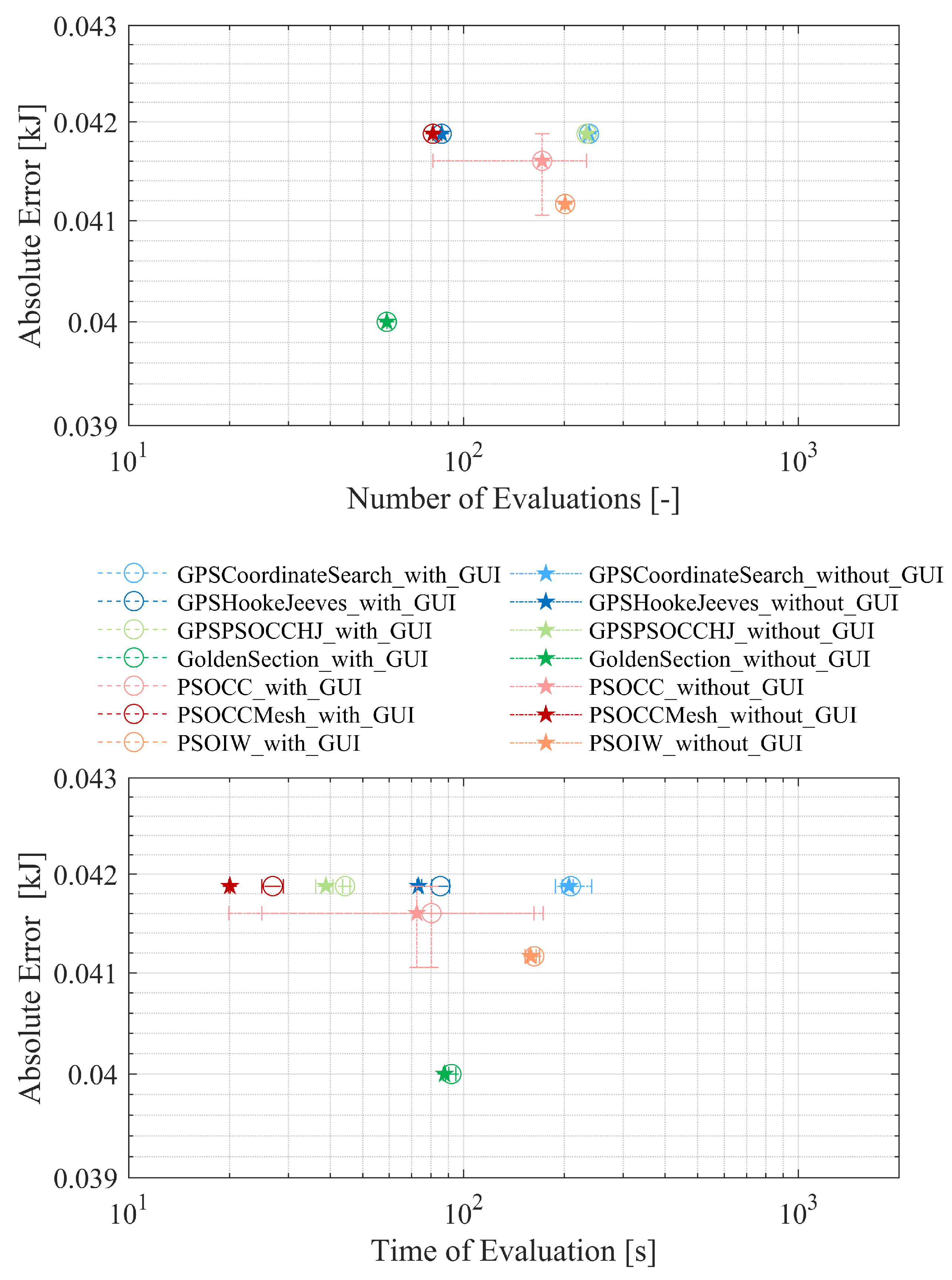
Each solver has a loop of three complete optimization cycles. Out of these three result sets, mean, minimum and maximum values were identified. In Figure 7, mean values and the minimum and maximum values as deviations are presented. Note, that the abscissa is in logarithmic scale.
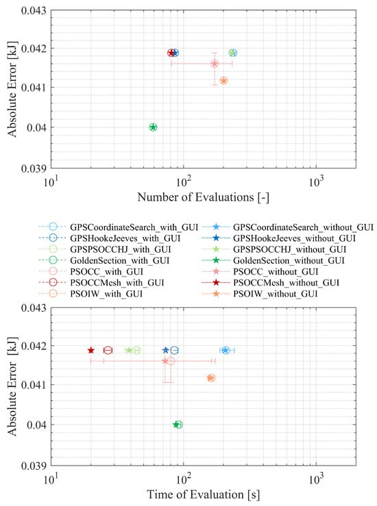
Figure 7.
GenOpt optimization results.
As these results show (Figure 7), the Particle Swarm Optimization algorithm with Constriction Coefficient and continuous independent variables restricted to a Mesh (PSO-CCMesh) performs best for the given constraints and problem formulation. Mean optimization time for PSO-CCMesh is about 26 s. It takes nearly half the time compared to the second fastest solver, Hooke–Jeeves Generalized Pattern Search implementation combined with leaded Particle Swarm Optimization algorithm with Constriction Coefficient (GPS-PSOCCHJ), with 44 s. PSO-CCMesh also has fewer iteration loops (81) than GPS-PSOCCHJ (233). PSO-CC, GPSHookeJeeve and Golden Section are about the same, with values between 72 and 87 s, and PSO-IW and GPSCoordinateSearch are far behind in last place with values of approx. 162 and 209 s. PSO-CC and GPS-PSOCCHJ also show higher fluctuations in the evaluation time, while the other solvers show relatively constant times.
By running GenOpt without a GUI, optimization time could be shortened to between 2 s (GPSCoordinateSearch) and 11 s GPSHookeJeeve in absolute values or between (GPSCoordinateSearch) and (PSO-CCMesh).
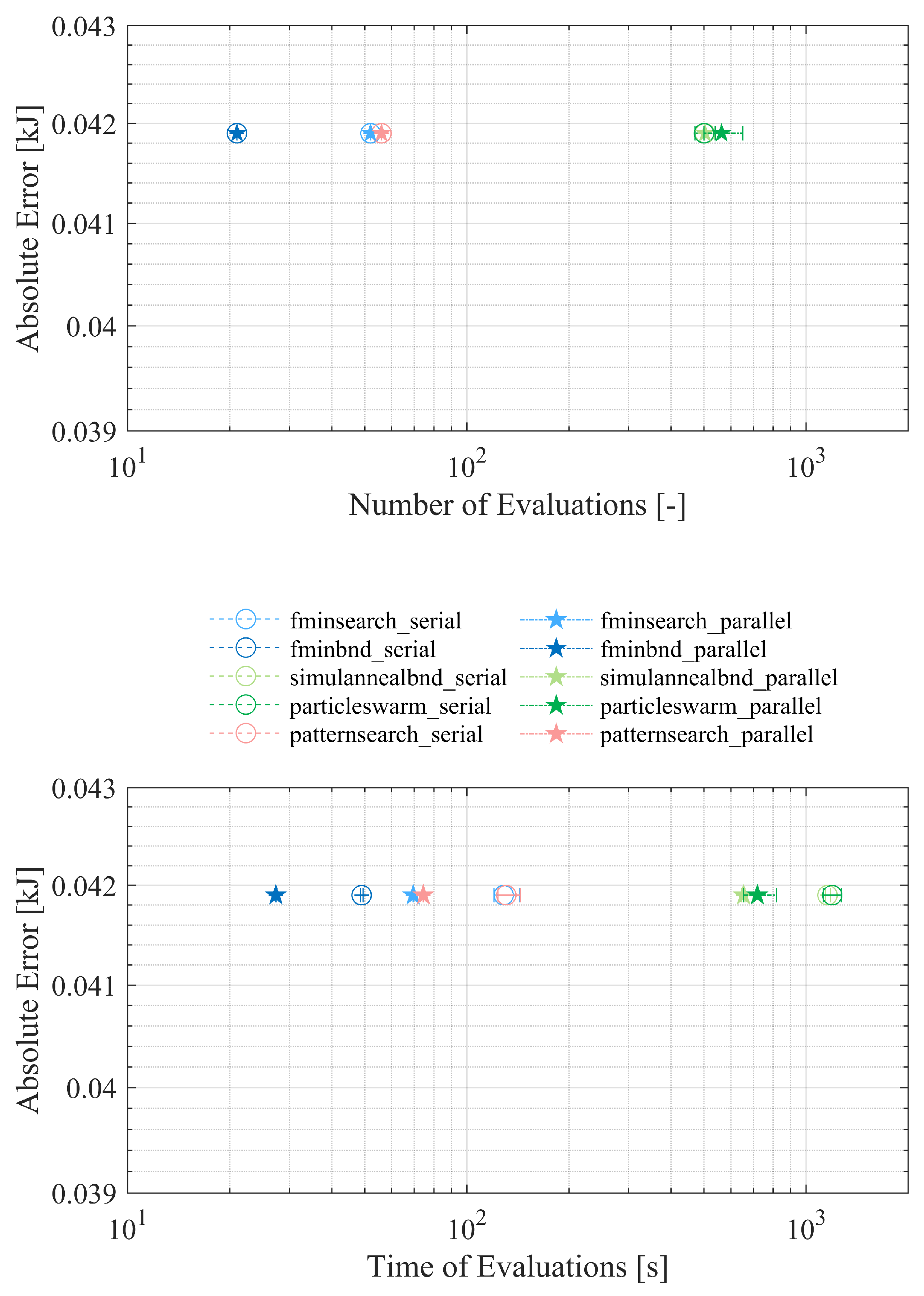
In MATLAB, nine solvers were taken into account (Table 5):
Table 5.
Individual solver boundaries in MATLAB.
- Find minimum of unconstrained multivariable function using derivative-free method (fminsearch).
- Find minimum of single-variable function on fixed interval (fminbnd).
- Particle Swarm Optimization (particleswarm).
- Simulated annealing algorithm (simulannealbnd).
- Pattern search algorithm (patternsearch).
- Genetic Algorithm (ga).
- Find minimum of constrained nonlinear multivariable function (fmincon).
- Find global minimum (GlobalSearch).
- Find multiple local minima (MultiStart).
Note that the solvers fminbnd and fminsearch do not require the Optimization Toolbox license. Their configuration can be performed by using the optimset function instead of optimoptions. Global search, multistart, Genetic Algorithm, particleswarm, simulated annealing and patternsearch are global optimizers. By giving a MATLAB function handle to a local solver such as fminsearch, they could optionally become a hybrid solver.
Mean objective values of solvers fmincon, ga, GlobalSearch and MultiStart are higher than the chosen upper limit of 0.05 kJ. They are in the range of 0.061 kJ (MultiStart) to 3300 kJ (ga).
Solver fminbnd, which is a one-dimensional optimizer for a bounded problem, performs best for the described problem. As the results, given in Figure 8, show, it takes 21 iteration loops and 48 s in serial mode and 27 s in parallel mode, respectively, which is nearly faster than in serial mode. Due to processing overhead in establishing the pool communication environment, the benefit in time savings is less than the linear behavior between the number of used processor cores and the optimization time. With average values between 54 and 74 s in parallel mode (107 to 130 s in serial mode), the solvers fmincon, fminsearch and patternsearch are in the midrange; GlobalSearch is behind with 289 s in parallel mode (382 s in serial mode); MultiStart, simulanneal and particleswarm follow with times between 500 and 718 s or 1156 and 1335 s in serial mode; and ga is in last place with times of over 2700 and 6300 s, respectively. Since global search, multistart, Genetic Algorithm and particleswarm are stochastic—that is, they make random initial guesses and choices—the number of evaluations changes in every optimization loop.
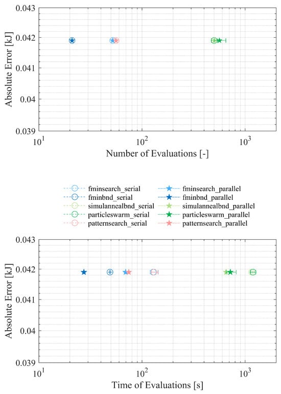
Figure 8.
MatOpt optimization results.
As noted before, the MATLAB solvers fmincon, ga, multistart and global search have a poor objective value. In direct comparison to the results of GenOpt’s mode without GUI and MATLAB in parallel mode, the remaining solvers have nearly the same objective value; GenOpt’s Particle Swarm Optimizer with Constriction Coefficient and continuous independent variables restricted to Mesh (PSOCCMesh) performs best among all considered solvers regarding time of evaluation. In the meantime, it takes 20 s compared to the second one, MATLAB’s fminbnd solver, which needs 27 s in mean and parallel modes (Figure 8).
5. Conclusions and Outlook
This benchmark study aims at comparing the numerical performance of GenOpt and MATLAB solvers for the identification of the overall heat transfer coefficient of a TRNSYS heat exchanger model. Four modes were implemented and investigated: GenOpt with a GUI and without a GUI, and MATLAB in serial optimization and in parallel optimization using the Parallel Computing Toolbox. Considering GenOpt, an interesting finding is that running without a GUI gives better performance, while MATLAB is faster in parallel mode, as was expected. The MATLAB solvers fmincon, ga, multistart and global search have a poorer objective value, while remaining solvers have nearly the same objective value. Hiding the GenOpt GUI increased the performance of solving the considered optimization problem up to (PSO-CCMesh) compared to the time with a GUI. Running in this mode, the GenOpt solver PSO-CCMesh gave the best performance in optimization time with 20 s, followed by the MATLAB solver fminbnd (27 s) in parallel computing mode. The top two solvers from GenOpt and MATLAB were followed by GPS-PSOCCHJ with approx. 38 s and MATLAB’s fmincon (54 s) and fminsearch (69 s). These were followed by GenOpt’s PSO-CC (72 s) and GPSHookeJeeve (73 s). With an average value of 74 s, patternsearch was close behind. This was followed by the remaining three GenOpt solvers, and the remaining five MATLAB solvers bring up the rear. Furthermore, it can be seen that most GenOpt solvers reach a solution faster than most MATLAB solvers; in a direct comparison between GenOpt with a GUI and the serial mode in MATLAB, the difference was consistently between 0.86 (fastest solvers PSO-CCMesh/fminbnd) and 29.2 (slowest solvers GPSCoordinateSearch/ga).
In the end, and in order to answer the research question posed at the beginning, it can be said that for the continuous single-objective optimization problem considered here, it is better to take the simpler route of using GenOpt.
The results suggest that the advantage in terms of time savings is particularly noticeable for complex single-objective optimization problems, such as the design of BES, which require many iteration loops. There are also advantages in simulation time for single-objective optimization problems in the area of optimal control using model predictive control and moving horizon in BES. This aspect should be taken into account for hardware-in-the-loop applications where the control task must fulfill corresponding real-time conditions. As already mentioned at the beginning, GenOpt can only handle single-objective optimization problems, which is why the TRNSYS–MATLAB framework used shows advantages, preferably in a Pareto optimization. Furthermore, well-known commercial solvers such as Gurobi, MOSEK and CPLEX have not yet been taken into consideration. Both GenOpt and MATLAB allow the user to integrate custom solvers; while this is only possible directly in the Java programming language in GenOpt, MATLAB is more flexible due to the availability of C++, Fortran and Python interfaces. Furthermore, as an integrated development environment, MATLAB offers a wider range of application options for extending the framework. Possible use cases here would be the connection of databases, network communication and cloud services or hardware connections and digital twins. On the other hand, the comparison with a Python-based framework such as pytrnsys and corresponding solver packages (e.g., pymoo) is of particular interest. These aspects have already been partially addressed and will be considered in future work.
Author Contributions
Conceptualization, J.M. and G.F.; methodology, J.M.; software, J.M.; validation, J.M. and G.F.; formal analysis, G.F.; investigation, J.M.; resources, G.F.; data curation, J.M.; writing—original draft preparation, J.M. and G.F.; writing—review and editing, J.M. and G.F.; visualization, J.M.; supervision, G.F. All authors have read and agreed to the published version of the manuscript.
Funding
This research received no external funding.
Data Availability Statement
Data are contained within the article.
Conflicts of Interest
The authors declare no conflicts of interest.
List of Acronyms
| ANN | Artificial Neural Network |
| BACS | Building Automation and Control System |
| BCVTB | Building Controls Virtual Test Bed |
| BES | Building Energy Systems |
| BPST | Building Performance Simulaton Tool |
| CFFI | C Foreign Function Interface |
| COM | Component Object Model |
| DLL | Dynamic Link Library |
| EPBD | Energy Performance of Buildings Directive |
| FIO | File Input/Output |
| FMI | Functional Mock-up Interface |
| FMU | Functional Mock-up Unit |
| GA | Genetic Algorithms |
| GEG 2023 | Building Energy Act |
| GenOpt | Generic Optimization Program |
| GPS | Generalized Pattern Search |
| GPSCS | Generalized Pattern Search Coordinated Search |
| GPS-PSOCCHJ | Generalized Pattern Search–Particle Swarm Optimization algorithm with Constriction Coefficient as particle update equation |
| GUI | Grapical User Interface |
| HVAC | Heating, Ventilation and Air Conditioning |
| IDAICE | IDA Indoor Climate and Energy |
| IEASHC | International Energy Agency Solar Heating and Cooling |
| LabVIEW | Laboratory Virtual Instrumentation Engineering Workbench |
| MATLAB | MATrix LABoratory |
| MOPSO | MOPS]Multiobjective Particle Swarm Optimization |
| MPC | Model Predictive Controller |
| NSGA-II | Nondominated Sorting Genetic Algorithm 2 |
| OPC UA | Open Platform Communications Unified Architecture |
| PCM | Phase Change Material |
| PSO | Particle Swarm Optimization |
| PSO-CC | Particle Swarm Optimization algorithm with Constriction Coefficient |
| PSO-CCMesh | Particle Swarm Optimization algorithm with Constriction Coefficient restricted to Mesh |
| PSO-IW | Particle Swarm Optimization algorithm with Inertia Weighting |
| RE | Renewable Energies |
| TCP/IP | Transmission Control Protocol/Internet Protocol |
| TRNSYS | TRaNsient SYstem Simulation Program |
References
- Wang, H.; Zhai, Z.J. Advances in building simulation and computational techniques: A review between 1987 and 2014. Energy Build. 2016, 128, 319–335. [Google Scholar] [CrossRef]
- Crawley, D.B.; Hand, J.W.; Kummert, M.; Griffith, B.T. Contrasting the capabilities of building energy performance simulation programs. Build. Environ. 2008, 43, 661–673. [Google Scholar] [CrossRef]
- EN 15232-1:2017; Energy Performance of Buildings—Energy Performance of Buildings—Part 1: Impact of Building Automation, Controls and Building Management—Modules M10-4,5,6,7,8,9,10. European Committee for Standardization: Brussels, Belgium, 2017.
- Federation of European Heating, Ventilation and Air Conditioning Associations (REHVA). EPB (Energy Performance of Buildings) Standards. 2024. Available online: https://www.rehva.eu/activities/epb-center-on-standardization/epb-standards-energy-performance-of-buildings-standards (accessed on 6 November 2024).
- Allegrini, J.; Orehounig, K.; Mavromatidis, G.; Ruesch, F.; Dorer, V.; Evins, R. A review of modelling approaches and tools for the simulation of district-scale energy systems. Renew. Sustain. Energy Rev. 2015, 52, 1391–1404. [Google Scholar] [CrossRef]
- Modelica Association. FMI-Functional Mock-Up Inferface—The Leading Standard to Exchange Dynamic Simulation Models. 2024. Available online: https://fmi-standard.org/ (accessed on 6 December 2024).
- Shao, X.; Ringsberg, J.W.; Johnson, E.; Li, Z.; Yao, H.D.; Skjoldhammer, J.G.; Björklund, S. An FMI-based co-simulation framework for simulations of wave energy converter systems. Energy Convers. Manag. 2025, 323, 119220. [Google Scholar] [CrossRef]
- Wolf, C.; Schleipen, M.; Frey, G. Secure Exchange of Black-Box Simulation Models using FMI in the Industrial Context. In Proceedings of the 15th International Modelica Conference 2023, Aachen, Germany, 9–11 October 2023; pp. 487–496. [Google Scholar] [CrossRef]
- Solar Energy Laboratory, University of Wisconsin. TRNSYS—A Transient System Simulation Program, Version: 17.02; Solar Energy Laboratory, University of Wisconsin: Madison, WI, USA, 2014.
- The MathWorks Inc. MATLAB, Version: 9.3 (R2017b); The MathWorks Inc.: Natick, MA, USA, 2017. Available online: https://www.mathworks.com (accessed on 9 December 2024).
- Wetter, M. GenOpt—A Generic Optimization Program. In Proceedings of the 7th International Buildings Simulation Conference, Rio de Janeiro, Brazil, 13–15 August 2001. [Google Scholar]
- Gomes, C.; Thule, C.; Broman, D.; Larsen, P.G.; Vangheluwe, H. Co-simulation: State of the art. arXiv 2017, arXiv:1702.00686. [Google Scholar] [CrossRef]
- Sagerschnig, C.; Gyalistras, D.; Seerig, A.; Prívara, S.; Cigler, J.; Vana, Z. Co-simulation for building controller development: The case study of a modern office building. In Proceedings of the International Conference–Cleantech for Sustainable Buildings. CISBAT, Lausanne, Switzerland, 14–16 September 2011; pp. 955–960. [Google Scholar]
- Engel, G.; Schweiger, G. A comparison of co-simulation interfaces between Trnsys and Simulink: A thermal engineering case study. In Proceedings of the 9th International Conference on Mathematical Modelling. MATHMOD, Vienna, Austria, 21–23 February 2018; pp. 47–48. [Google Scholar] [CrossRef]
- Trcka, M. Co-Simulation for Performance Prediction of Innovative Integrated Mechanical Energy Systems in Buildings. Ph.D. Thesis, University of Technology, Eindhoven, The Netherlands, 2008. [Google Scholar] [CrossRef]
- Widl, E. The FMI++ TRNSYS FMU Export Utility. 2022. Available online: https://github.com/fmipp/trnsys-fmu (accessed on 15 November 2024).
- Widl, E.; Müller, W. Generic FMI-compliant Simulation Tool Coupling. In Proceedings of the 12th International Modelica Conference, Prague, Czech Republic, 15–17 May 2017; pp. 321–327. [Google Scholar] [CrossRef]
- Wetter, M. A Modular Building Controls Virtual Test Bed for the Integrations of Heterogeneous Systems. Ph.D. Thesis, Lawrence Berkeley National Laboratory, Berkeley, CA, USA, Oak Ridge, TN, USA, 2008. [Google Scholar]
- Pan, Y.; Lin, X.; Huang, Z.; Sun, J.; Ahmed, O. A verification test bed for buildingcontrol strategy coupling TRNSYS with a real controller. In Proceedings of the 12th Conference of International Building Performance Simulation Association. IBPSA, Sydney, Australia, 14–16 November 2011; pp. 215–222. [Google Scholar]
- Junge, M. Simulationsgestützte Entwicklung und Optimierung Einer Energieeffizienten Produktionssteuerung. Ph.D. Thesis, Kassel University, Kassel, Germany, 2007. [Google Scholar]
- Riederer, P.; Keilholz, W.; Ducreux, V. Coupling of TRNSYS with Simulink—A method to automatically export and use TRNSYS models within Simulink and vice versa. In Proceedings of the 11th International Buildings Simulation Conference, Glasgow, UK, 27–30 July 2009. [Google Scholar]
- Al-Saadi, S.N. Modeling and Simulation of PCM-Enhanced Facade Systems. Ph.D. Thesis, University of Colorado at Boulder, Boulder, CO, USA, 2014. [Google Scholar]
- Bernier, N.; Marcotte, B.; Kummert, M. Calling Python from TRNSYS with CFFI. 2022. Available online: https://www.trnsys.de/addons (accessed on 6 November 2024).
- Institute for Solar Technology (SPF)-Eastern Switzerland University of Applied Sciences (OST). Pytrnsys: The Python TRNSYS Tool Kit. 2022. Available online: https://pytrnsys.readthedocs.io/en/latest/ (accessed on 6 November 2024).
- Solmaz, A.S. A critical review on building performance simulation tools. Alam Cipta 2019, 12, 7–21. [Google Scholar]
- Barber, K.A.; Krarti, M. A review of optimization based tools for design and control of building energy systems. Renew. Sustain. Energy Rev. 2022, 160, 112359. [Google Scholar] [CrossRef]
- Kalkan, C.; Ward, C.; Duquette, J.; Khouli, F.; Ezan, M.A. Lessons Learned From Modelling a Complex Residential Building Energy System in TRNSYS. In Proceedings of the 13th eSim Building Simulation Conference 2024. IBPSA, Edmonton, AB, Canada, 5–7 June 2024. [Google Scholar]
- Nayak, A.K.; Hagishima, A. Modification of building energy simulation tool TRNSYS for modelling nonlinear heat and moisture transfer phenomena by TRNSYS/MATLAB integration. E3S Web Conf. 2020, 172, 25009. [Google Scholar] [CrossRef]
- Mazzeo, D.; Matera, N.; Cornaro, C.; Oliveti, G.; Romagnoni, P.; De Santoli, L. EnergyPlus, IDA ICE and TRNSYS predictive simulation accuracy for building thermal behaviour evaluation by using an experimental campaign in solar test boxes with and without a PCM module. Energy Build. 2020, 212, 109812. [Google Scholar] [CrossRef]
- Magni, M.; Ochs, F.; de Vries, S.; Maccarini, A.; Sigg, F. Detailed cross comparison of building energy simulation tools results using a reference office building as a case study. Energy Build. 2021, 250, 111260. [Google Scholar] [CrossRef]
- Asadi, E.; da Silva, M.G.; Antunes, C.H.; Dias, L. A multi-objective optimization model for building retrofit strategies using TRNSYS simulations, GenOpt and MATLAB. Build. Environ. 2012, 56, 370–378. [Google Scholar] [CrossRef]
- Magnier, L.; Haghighat, F. Multiobjective optimization of building design using TRNSYS simulations, genetic algorithm, and Artificial Neural Network. Build. Environ. 2010, 45, 739–746. [Google Scholar] [CrossRef]
- Fernandes, M.; Gaspar, A.; Costa, V.; Costa, J.; Brites, G. Optimization of a thermal energy storage system provided with an adsorption module—A GenOpt application in a TRNSYS/MATLAB model. Energy Convers. Manag. 2018, 162, 90–97. [Google Scholar] [CrossRef]
- Narayanan, M.; Lima, A.F.d.; de Azevedo Dantas, A.F.O.; Commerell, W. Development of a Coupled TRNSYS-MATLAB Simulation Framework for Model Predictive Control of Integrated Electrical and Thermal Residential Renewable Energy System. Energies 2020, 13, 5761. [Google Scholar] [CrossRef]
- Mylonas, A.; Macià-Cid, J.; Péan, T.Q.; Grigoropoulos, N.; Christou, I.T.; Pascual, J.; Salom, J. Optimizing Energy Efficiency with a Cloud-Based Model Predictive Control: A Case Study of a Multi-Family Building. Energies 2024, 17, 5113. [Google Scholar] [CrossRef]
- Arenas-Larrañaga, M.; Gurruchaga, I.; Carbonell, D.; Martin-Escudero, K. Performance of solar-ice slurry systems for residential buildings in European climates. Energy Build. 2024, 307, 113965. [Google Scholar] [CrossRef]
- Meiers, J.; el Jeddab, A.; Theis, D.; Jonas, D.; Frey, G.; Deissenroth-Uhrig, M. Hardware-in-the-loop integration of PVT models using Internet of Things-enabled communication. In Proceedings of the ISES and IEA SHC International Conference on Solar Energy for Buildings and Industry, Eurosun, Kassel, Germany, 25–29 September 2022. [Google Scholar] [CrossRef]
- National Instruments Corp. LabVIEW—Laboratory Virtual Instrumentation Engineering Workbench; National Instruments Corp.: Austin, TX, USA, 2018. [Google Scholar]
- Tadayon, L.; Meiers, J.; Jonas, D.; Frey, G. Design of a building energy system using model-based multi-objective optimization. In Proceedings of the PESS 2023, Power and Energy Student Summit, Bielefeld, Germany, 15–17 November 2023; pp. 49–55. [Google Scholar]
Disclaimer/Publisher’s Note: The statements, opinions and data contained in all publications are solely those of the individual author(s) and contributor(s) and not of MDPI and/or the editor(s). MDPI and/or the editor(s) disclaim responsibility for any injury to people or property resulting from any ideas, methods, instructions or products referred to in the content. |
© 2025 by the authors. Licensee MDPI, Basel, Switzerland. This article is an open access article distributed under the terms and conditions of the Creative Commons Attribution (CC BY) license (https://creativecommons.org/licenses/by/4.0/).