Abstract
A jet flow mixer is a novel agitator type widely used in the industry. However, scientific research has yet to be conducted on this impeller type. In this study, six types of fluids with various properties widely used in the paint industry were chosen to calculate the positioning of the jet flow mixer in the tank. Calculations were performed using computational fluid dynamics (CFD) software and validated using literature data. Simulations were conducted to consider the inside of the jet flow mixer and the inside of the tank. The initial calculations made for jet flow mixers allowed the determination of volume flow and power numbers for three types of mixers (propeller agitator and Pitched Blade Turbine with three and four blades). Those parameters were then used in subsequent calculations, obtaining the optimal inclination angle of the agitator and power consumption for each considered case. The jet flow mixer with a propeller impeller positioned at an angle of 45° proved to be the choice to achieve the best results.
1. Introduction
Jet flow mixers are modern solutions for various chemical processes such as mixing, homogenisation, emulsification, dispersion, etc. Some of these processes need the mixing of Newtonian, non-Newtonian, or highly viscous fluids, essential in the paint, varnish, chemical, food, and pharmaceutical industries. A jet flow mixer combines a rotor–stator mixer, axial impeller (propeller or PBT), and a traditional jet mixer.
In the design of a jet flow mixer, axial agitators are used, considering its advantages of large flow and good pumping performance [1]. Axial impellers create two fluid flow loops, efficiently mixing the tank’s lower and upper parts [2]. Propeller impellers are commonly used in industries, especially when keeping particles suspended in a liquid [3]. Another widely used axial impeller is the Pitched Blade Turbine (PBT). This impeller can generate higher volume flows than a propeller agitator; however, it requires more energy [4,5]. When designing a mixing tank, it is essential to consider different geometries of impellers. Wider blades on a propeller impeller can be more effective than Rushton or PBT impellers with less energy consumption [6]. The effectiveness of mixing in a stirred tank depends on the stirrer’s installation in the tank [7,8], stirrer geometry [9,10], rotational speed of the impeller [11], presence and geometry of baffles [12,13], and type of fluid [14,15].
The main advantage of a traditional jet mixer is its lack of moving parts, which makes it cheap and easy to install. For mixing with a jet mixer, the liquid is drawn into a pump and then released to the tank under pressure through the jet nozzle. The stream flows across the tank and creates two main circulation loops. The efficiency of the jet mixer depends on the fluid discharge velocity [16], angle of the nozzle [17], jet location [18], and geometry of the tank [19] and tank bottom [20]. Studies have also shown that positioning two jet mixers inside a tank is more effective than using one jet mixer [18]. The position of a second jet mixer in the tank was also investigated, shortening the mixing time through proper positioning [21,22]. A jet mixer can be added to the tank with an axial impeller, increasing the mixing [2].
Rotor–stator mixers (RSMs), also called high shear mixers (HSMs), consist of a mixing element called a rotor and a fixed element called a stator. The gap between the rotor and stator is small (100–300 µm) [4,23]. The mixing element rotates at a high rotational speed (10–50 m/s) [4,23,24]. Due to these features, rotor–stators produce high local shear rates, making possible the deagglomeration, emulsification, and homogenisation processes used in various chemical industries such as paint, cosmetics, or food [4,25]. Several geometries of rotor–stator are available (colloid mills and toothed devices, radial discharge impellers, or axial discharge impellers) depending on the desired results [4]. Whether the flow will be axial or radial relies on the geometry of the stator [4,26]. Moreover, a rotor–stator can be operated in batch, semi-batch, and continuous (inline) modes. Performing a constant process is desirable due to economic advantages. However, predicting the power consumption of an inline rotor–stator is much more complex than for the batch process [27], making it hard to predict the final operational cost.
Combining the three main mixer types allows us to take full advantage of each option’s benefits. In a jet flow mixer, the rotor draws fluid into the mixing area and draws the fluid out in the axial direction. The fluid flow is possible due to the rotor’s pressure gradient, making it unnecessary to use the pump. The generation of a high-volume fluid flow is possible by using an axial impeller without the possibility of clogging the nozzle (in the case of a suspension fluid). The unique geometry of the jet flow mixer creates a circulation loop without creating a vortex, which reduces the possibility of air being mixed into the fluid. Moreover, correctly positioning the mixer in the tank prevents the settling of suspended particles.
Assessment of fluid flow in the mixers, especially near the mixer, can be performed using experimental and simulation methods. For experimental determination of fluid flow characteristics, Laser Doppler Anemometry (LDA) [28,29] and Particle Image Velocimetry (PIV) [30,31] were used. The experimental results validated the simulation performed using computational fluid dynamics. CFD calculations often use the RANS Standard k-ε model [32,33] and the Realisable k-ε model [27,30]. To validate the results, a comparison of shaft power [34], residence time [35], and mixing efficiency [33] was performed.
In this study, calculations were performed for a plant tank with a jet flow mixer. The calculations were divided into two parts. In Step I, the flow rate through the jet flow mixer was calculated by determining the rotational speed of the agitator. This calculation allowed us to assess flow rates through the jet flow mixer, which was then used to model the fluid flow in the tank (Step II). Dividing the calculations into two stages allowed the creation of a fine calculation grid (necessary to model the flow in the mixer) and a coarser calculation grid to model fluid flow in the tank. This approach made it possible to increase the accuracy of calculations while reducing computational power and time. Calculations were performed for five types of liquids used in the paint and varnish industry. The aim of this paper is to determine the optimal positioning of the jet flow mixer in the tank.
2. Materials and Methods
2.1. Mathematical Modelling
2.1.1. Geometry
Two geometries were created to perform calculations. For Step I of the calculations, the geometry of the jet flow mixer was created. For Step II, the geometry of the plant tank was used. Figure 1 presents geometries used in calculations.
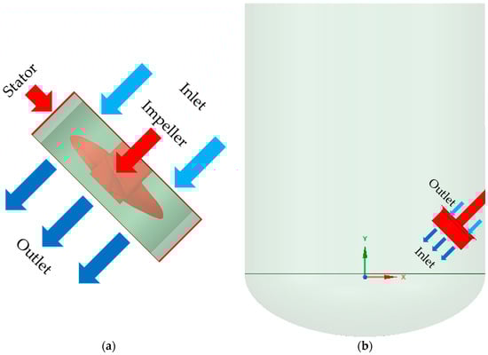
Figure 1.
Geometries for calculations (a) in Step I (dark green colour represents interface between inner and outer region for correct use of MRF) and (b) in Step II.
Step I: In this study, three types of agitators in the jet flow mixer were used: a propeller impeller with three blades (case 1) and Pitched Blade Turbines with three (case 2) and four (case 3) blades. The stator diameter was 0.538 m, and its height was 0.180 m. The diameter of the rotor was 0.4 m, and its height was 0.1 m. The geometries of the agitators used are presented at Figure 2.
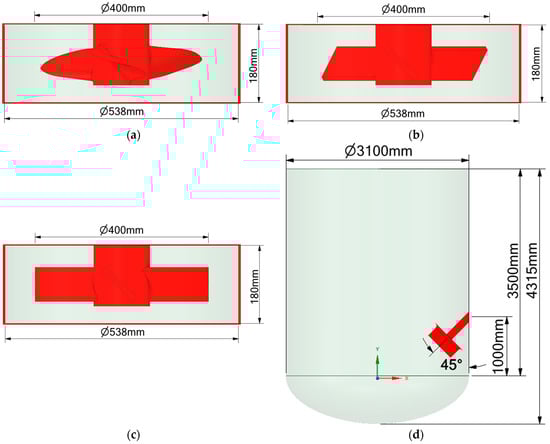
Figure 2.
The geometries of three types of impellers: (a) a propeller impeller (case 1), (b) a PBT with three blades (case 2), (c) a PBT with four blades (case 3), (d) the tank’s geometry with a jet flow mixer positioned at a 45° angle. The red surface represents the walls of the jet flow mixer.
Step II: The jet flow mixer was placed in the reaction tank. The geometry represents the inner tank volume available for the modelled fluid. The tank is a cylindrical tank (3.1 m in diameter and 3.5 m in height) with an ellipsoidal bottom (0.815 m in height) and a capacity of 30 m3. The jet flow mixer was placed in the tank at an angle through the side wall, one metre above the bottom of the cylindrical part of the tank. In all calculations, the centre of the inlet to the tank was fixed 0.5 m from the wall of the tank. The outlet from the tank was placed perpendicular to the inlet at a distance of 0.180 m, while its position relative to the wall and the length of the shaft were functions of the angle of inclination of the impeller. Calculations were performed for four angles of agitator inclination: 45°, 33°, 30°, and 27°. Angles of inclination were chosen based on literature data for traditional jet mixers. The data states that the best mixing is observed with an angle inclination of 45° [17]; however, mixing was faster with an angle of inclination of 30° [18,36]. The data were obtained for traditional jet mixers, not for the jet flow mixer. Therefore, multiple angles of inclination around the best results were chosen to perform a calculation for the new type of mixer. The geometry of the tank with the jet flow mixer is presented at Figure 2.
2.1.2. Mesh
Step I: The mesh was generated using Fluent Meshing from ANSYS 2024R1. The jet flow mixer mesh was adjusted to the Multiple Reference Frame (MRF) model setting to model fluid flow through the agitator. Five boundary layers and poly-hexcore elements were used to create the mesh. The calculations were performed for three mesh densities of about 116,000, 287,000, and 512,000 elements. The difference in results between the least and most dense mesh was 3%, and the difference between the meshes with 287,000 and 512,000 elements was less than one percent. Based on the results, it was decided to use a mesh of 287,000 elements for further calculations. This allowed for a decrease in calculation time. The mesh was created from cells with a maximum size of 8 mm and a minimum size of 0.5 mm.
Step II: Meshes with about 2.2 million, 4 million, and 4.7 million elements were created to model fluid flow in the tank properly. The difference in results between the least and most dense mesh was 25%, and the difference between the meshes with 4 and 4.7 million elements was less than one percent. To reduce calculation time, it was decided to use a mesh of 4 million elements for further calculations. Five boundary layers and poly-hexcore elements were used. The mesh was created from cells with a maximum size of 30 mm and a minimum size of 0.1 mm.
2.1.3. Boundary Condition
Simulations were performed using ANSYS Fluent 2024R1. Step I: The turbulence model used for modelling fluid flow through the agitator was the SST k–ω model. The SST k–ω model was chosen as it is used for turbulent flows (with significant vortices and recirculation zones) that require accurate modelling of near-wall regions for detailed representation of velocity gradient and turbulence parameters. The model has been successfully used to model fluid flow in both axial impeller [37,38] and rotor–stator mixers [30,39]. Simulations were performed in a stationary state. The Multiple Reference Frame model correctly models flow patterns and characteristics. This model is used when modelling multiple moving parts of a geometry, for example, impellers and pumps, when the fluid flow is stationary. When using the MRF model, the computational domain is divided into cell zones with different rotational or transitional speeds, creating stationary and rotating frames. This model allows the recreation of the movement of the blades of the agitator with a no-slip condition on the walls [40,41]. The MRF model is widely used to model the rotation of impellers [42,43,44]. The interface between the inner rotating region (surrounding the rotor) and the outer stationary region (surrounding the stator) is indicated at Figure 1. For the calculations, the rotational speed of the agitator was equal to 1500 rpm. The direction of rotation was clockwise. At the inlet, a pressure inlet boundary condition was applied. The gauge pressure was calculated as the height of the liquid column above the agitator. The values of gauge pressure are shown in Table 1. A pressure outlet boundary condition was applied to the outlet. The same gauge pressure was used at the outlet as at the inlet.

Table 1.
The gauge pressure applied at the inlet and outlet to the tank.
Step II: A Standard k-ε model with Standard Wall Functions was used to model fluid flow in the tank. The Standard k-ε model was chosen as it is used to model fully turbulent flow well away from walls (near-wall resolutions are less critical). This model is often used to model mixing in a tank [32,33]. The inlet to the tank was located at the outlet of the agitator. The mass flow inlet boundary condition was applied to perform the calculations. The mass flow at the inlet to the tank was the same as the mass flow of the fluid at the outlet of the agitator. The outlet from the tank was located at the inlet to the mixer. An outflow condition was used at the outlet. The outflow boundary condition allows you to model flow outlets when details about flow velocity and pressure are unknown [41]. The wall of the tank and the outer wall of the mixer were modelled as moving walls with speeds of 0 m/s and no-slip conditions.
The SIMPLE pressure–velocity coupling scheme and Second-Order Upwind Discretisation were used to solve the calculations. The calculations were performed under stationary conditions.
2.2. Rheology
Calculations were performed for five types of fluid: water, industrially significant suspension (ISS), industrially significant resin (ISR), calcium carbonate suspension, and titanium dioxide suspension. Calculations were performed for fluid flow at 20 °C. Additionally, due to the significant decrease in viscosity with the increasing temperature of the industrially significant resin, measurements at two temperatures were performed. ISR is used in industrial processes whose temperatures range from 20 °C to 60 °C. Therefore, it was decided that viscosity measurements and subsequently CFD calculations for ISR would also be performed at 60 °C (ISR60). The viscosities of the industrially significant resin and industrially significant suspension were measured using a Modular Compact Rheometer designed by Anton Paar and the coaxial cylinder system. The measurements were performed for the range of shear stress from 0.1 to 1000 s−1 at 20 °C (and for ISR additionally for 60 °C), and for every temperature, measurements were performed six times for three samples. From the results obtained, the average values were drawn out.
When performing the rheological measurements, it was assumed that the shear rate in the system would not exceed 1000 s−1. After performing the calculations from Step I, the accuracy of this assumption was checked. In each case, the fluid volumes with shear rate values exceeding 1000 s−1 were less than 3% of the system volume. Therefore, it can be concluded that the assumption made is correct.
2.2.1. Water
The physicochemical properties of water were uploaded from the Fluent Database. At 20 °C, the viscosity of water is 0.001003 Pa·s and the density of water is 998.2 kg/m3.
2.2.2. Industrially Significant Resin
The tested resin is a significant component for many products in the paint industry. The viscosity measurements were performed as described above. The investigation showed that the ISR was a Newtonian fluid with an average of 5.48 Pa·s viscosity at 20 °C and 0.36 Pa·s at 60 °C. The main component of the resin is water, which led to the assumption that the density of the ISR is equal to the density of the water and is 998.2 kg/m3. Figure 3 shows the rheological model’s fit to the ISR experimental data.
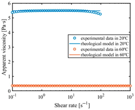
Figure 3.
The rheological model’s fit to the ISR experimental data.
2.2.3. Industrially Significant Suspension
The tested suspension was a silicate suspension with many applications in the paint industry. The measurements performed for this study indicated that the ISS was a shear-thinning liquid with an inflexion point at a shear stress of 10 s−1. It was assumed that solid particles suspended in a mixture of fluids could be described as a homogeneous substance. The viscosity curve of this suspension can be described using the Ostwald model. The rheological model Equations for the ISS can be described using a system of Equation (1).
where µ [Pa·s] is the apparent viscosity, [s−1] is the shear rate, k [Pa·sn] is the consistency flow index, and n [-] is the flow behaviour index. The lower values of the shear stress consistency flow index equal 20.903 Pa·sn, and the flow behaviour index equals 0.075. For shear stress values higher than 10 s−1, the consistency flow index is 5.497 Pa·sn, and the flow behaviour index is 0.653. The fit of the rheological model to the experimental data is shown at Figure 4. The density of the ISS was calculated as a harmonic mean of the density of its raw materials and was 1182.7 kg/m3.
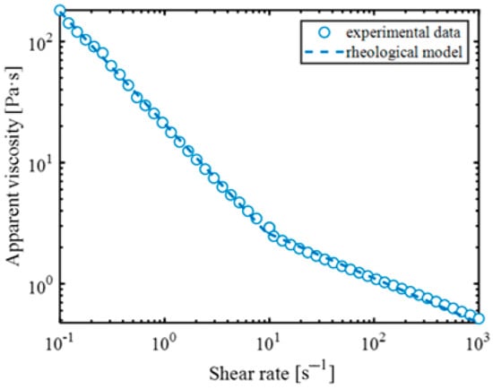
Figure 4.
The rheological model’s fit to the ISS experimental data.
2.2.4. Calcium Carbonate Suspension
An aqueous suspension of calcium carbonate is another crucial component in the paint industry. In the calculations, it was assumed that the suspension consisted of 70% calcium carbonate and 30% water by mass. The density of the calcium carbonate suspension was calculated as the harmonic mean of the density of the raw materials and was 1789.2 kg/m3.
The viscosity of the calcium carbonate was calculated based on the data published in [45]. The published data suggest that calcium carbonate suspension is a fluid with shear-thinning to shear-thickening properties. The behaviour of the liquid changes at the value of the shear stress threshold, equal to 610 s−1. For this reason, the viscosity curve should be described as a summary of two Equations. The Ostwald model can be applied to the higher values of shear stresses. The flow consistency index is 0.0047, and the flow behaviour index is 2.428. For shear stresses lower than 610 s−1, the Bingham model [46] can be used, as described by Equation (2).
where τ0 [Pa] is the Bingham yield stress, µpl [Pa·s] is the plastic viscosity index, and n [-] is the flow behaviour index. For this study, the Bingham yield stress is 5.016 Pa, the plastic viscosity is 0.066 Pa·s, and the flow behaviour index is 1. The fit of the rheological model to the experimental data is shown at Figure 5. It was assumed that solid particles suspended in a mixture of fluids could be described as a homogeneous substance.
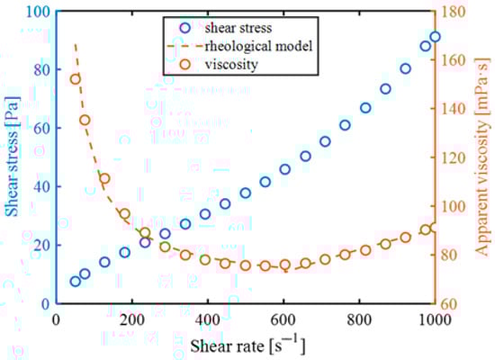
Figure 5.
The fit of the rheological model to the experimental data for the calcium carbonate suspension.
2.2.5. Titanium Dioxide Suspension
The aqueous titanium dioxide suspension consisted of 40% titanium dioxide and 60% water (by mass). The density of the calcium carbonate suspension was calculated as the harmonic mean of the density of the raw materials and was 1440 kg/m3.
The viscosity model used for the calculations was published in [47]. The published data suggest that titanium dioxide is a shear-thinning liquid, which can be described using the Carreau model [48], described by Equation (3).
where µ∞ = 0.11 Pa·s is the viscosity at the infinite shear rate, µ0 = 14.09 Pa·s is the viscosity at the zero shear rate, λ = 1.73 s is the relaxation time, and n = 0.1 is the flow index.
2.3. Power Consumption
Pumping numbers (NFl) and dimensionless power numbers (NP) were calculated to validate the calculations. A pumping number is a dimensionless number that determines fluid flow through the impeller. Its values depend on the geometry of the impeller and rotational speed. The calculated pumping number for each impeller was compared with the literature data. The pumping number was calculated using Equation (4).
where Q [m3/s] is the flow rate, N [s−1] is the rotational speed, and D [m] is the diameter of the impeller.
Power consumption depends on the properties of the fluid (its density and viscosity), the agitator’s rotational speed, and the agitator’s geometry. A dimensionless power number is used to compare power consumption for different impellers. Its value is experimentally determined and is dependent on the Reynolds number. The Reynolds number for impellers is defined by Equation (5).
where ρ [kg/m3] is the density of the fluid. For Newtonian fluids, viscosity is constant inside the tank. However, apparent viscosity must be calculated when performing power consumption calculations with non-Newtonian fluids. Metzner and Otto proposed a widely used method of calculating apparent viscosity [14]. This concept assumes that, in the stirred tank, the averaged shear rate is proportional to the impeller’s rotational speed, and is given by Equation (6):
where Ks is the Metzner–Otto constant, which depends on the impeller geometry. The Metzner–Otto constant was calculated according to the method described in [49]. The calculated values of the Metzner–Otto constant and the apparent viscosity calculated for the non-Newtonian fluids are presented in Table 2.
Table 2.
Values of Metzner–Otto constant and apparent viscosity calculated for considered non-Newtonian fluids.
In the tank without a vortex, the dimensionless power number changes its value with the Reynolds number for laminar and transitional flow (Re < 10,000) and is constant for turbulent flow. The values of the dimensionless power number can be found in the literature (described with the Reynolds Diagram) or experimentally determined. To experimentally determine the dimensionless turbulent power number, Equation (7) is used.
where NP [-] is the dimensionless power number characteristic of a given impeller.
Shaft power (P) was calculated to determine power consumption. The power applied to the impeller is equal to the power delivered to the fluid by the impeller blades moving at a certain speed. This power can be calculated using torque and is defined by Equation (8):
where M [N·m] is torque, and the torque value can be exported from CFD software (ANSYS Fluent 2024 R1).
3. Results
3.1. Step I
3.1.1. Velocity Field
To validate the obtained results, the flow pattern of water for each impeller was exported from the CFD software and is shown at Figure 6. Each impeller generated axial fluid flow (down the jet mixer). This axial flow is characteristic of the chosen mixers. Moreover, axial fluid flow is also typical for rotor–stators when there are no cavities in the stator, as the steep velocity gradients that spread radially are generated when the stator has cavities. The most intensive fluid flow for the propeller impeller was observed in the centre of the jet flow mixer. Near the walls of the stator, reversed flow was observed, resulting in a flow rate that was smaller than theoretical. This flow pattern is typical for considered impellers and was experimentally measured and visualised in [6].
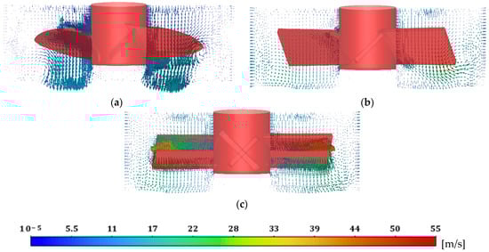
Figure 6.
Flow patterns generated (a) with propeller impeller (case 1), (b) with Pitched Blade Turbine with 3 blades (case 2), (c) with Pitched Blade Turbine with 4 blades (case 3).
The fluid velocity generated by the considered impellers was the highest for case 3 (descriptions of the cases can be found in the Materials and Methods Section in the Geometry Subsection). For this impeller, velocities as high as 55 m/s were observed at the impeller’s blades. The slowest fluid flow was generated in case 1. High velocities of the fluid are visible only on the blades of the mixer. This is another characteristic feature of axial impellers. The analysis of the fluid flow features generated by the axial impeller suggests that the liquid flow through the jet flow mixer is correct. Further investigation on validating the results is presented in the following subsection.
Fluid flow through the jet flow mixer was calculated for each considered fluid. Figure 7 shows the flow patterns generated by the propeller impeller for six fluids. The propeller impeller was chosen for flow pattern visualisation due to the popularity of its application in the industry. Similar fluid flow patterns were observed for each fluid. The differences in velocity at the blades of the impeller were noticed. The highest velocities were obtained for the suspensions and the lowest for ISR20.
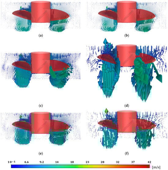
Figure 7.
Flow patterns generated for case 1 for six types of fluids: (a) water, (b) ISR20, (c) ISR60, (d) ISS, (e) calcium carbonate, and (f) titanium dioxide suspensions.
At Figure 7, recirculation areas were observed near the wall, under the blades. The most visible recirculation areas were noticed for water and ISR20. For other liquids, recirculation zones were observed; however, fluid flow was significantly lower. Moreover, dead zones under the agitator shafts were observed.
3.1.2. Flow Rate
Flow rate calculations were performed for each considered liquid and the three impellers. Volume flow through the jet flow mixer was generated using CFD software. Further validation of the obtained results was performed by comparing the calculated results to the theoretical data. Theoretical values of pumping numbers were calculated from the transformed Equation (4). The pumping number for the propeller impeller was taken from [50,51].
The volume flows through the jet flow mixer obtained from the CFD simulations are shown in Table 3 and are slightly lower than the theoretical values. The smallest flow generated in case 1 was obtained for ISR20. However, in cases 2 and 3, the smallest flow rate was obtained for ISS. For each impeller, the highest flow rate occurred for water. In each case, the calculated value of the flow rate is lower than the theoretical value. However, the values obtained from CFD refer to a jet flow mixer whose design differs from the geometry of the traditional axial mixer. The difference lies, among other things, in the ratio of the mixer’s diameter to the diameter of the tank or, as in the cases under consideration, the stator walls. This ratio is 1/3 in the traditional mixers, which is much more significant than in the cases under consideration. Such construction of the jet flow mixer causes the formation of recirculation zones (which can be observed at Figure 6 and Figure 7) in the area of the jet mixer, consequently lowering the liquid flow. However, given the insignificant differences in fluid flows, it can be assumed that the calculations were performed correctly.
Table 3.
Comparison of flow rates and pumping numbers obtained for three cases and six types of fluid (water, ISR20, ISR60, ISS, calcium carbonate suspension, and titanium dioxide suspension) with theoretical values.
When comparing flow rates for water obtained from theoretical correlation (Table 3) with the value generated from CFD software, the smallest value of relative error is obtained in case 2 and is 3%. These values are higher for cases 1 and 3, respectively, at 14% and 20%. Therefore, it can be assumed that the theoretical and simulated values are consistent.
Table 3 also compares values of pumping numbers found in the literature with the ones calculated using Equation (4). The computed pumping number values oscillate around the theoretical values and are proportional to the flow rate. The mean values in cases 1, 2, and 3 are 0.404, 0.550, and 0.598, respectively, and the relative errors are 27%, 18%, and 25%, respectively. Therefore, it can be assumed that the calculated pumping numbers are consistent with theoretical values and can be further used to describe fluid flow in the tank.
3.1.3. Power Number
Table 4 compares values of dimensionless power numbers for each impeller. Power consumption is needed to calculate the power number. Many researchers use shaft power, which can be estimated using Equation (8). Torque values were exported from CFD software. The higher the fluid density, the more torque is required to move the fluid. As a consequence, power consumption is also rising. The highest power consumption values for each impeller were obtained for calcium carbonate. Power consumption is the lowest in case 1 and the highest in case 3.
Table 4.
Comparison of shaft power and dimensionless power numbers obtained from CFD software for three cases and six types of fluid (water, ISR20, ISR60, ISS, calcium carbonate suspension, and titanium dioxide suspension).
The dimensionless power number was calculated using Equation (7). Mixing is performed in a turbulent regime based on the Reynolds number calculation inside the jet flow mixer. Therefore, it can be predicted that the obtained results of the power number should be constant. The results for each fluid slightly differ. For each impeller, the highest power number values were obtained for water, and the smallest values were obtained for ISS in cases 1 and 3 and for ISR60 in case 2. The relative error was calculated between the highest result (water) and the lowest result of the power number to estimate the difference in the results obtained for each liquid. The relative error is 7% in case 1, 18% in case 2, and 15% in case 3. Therefore, it can be assumed that the results are consistent and can be used to perform further calculations.
3.2. Step II
3.2.1. The Dependence of the Mixing Ratio on the Angle of Inclination of the Impeller
The effect of the inclination of the impeller on the mixing degree was investigated. Four angles of inclination were tested. The calculations were performed for the propeller agitator (case 1) since the highest ratio of flow rate to power consumption was obtained for this impeller. To start the calculation, the flow rate through the inlet to the tank has to be specified. The flow rate that enters the tank is the same as the flow rate that exits the jet flow mixer. The values of flow rates change with the properties of fluids. Therefore, the flow rates presented in Table 4 were chosen to perform further calculations.
To determine the dependence of the inclination of the impeller on the mixing ratio, ISR20 was chosen. This liquid was selected due to its importance in the industry, high viscosity, and easiness of implementation. The higher the fluid’s viscosity, the more challenging it is to mix due to the higher power consumption and difficulties with maintaining a high enough velocity of the fluid in the tank.
When choosing the inclination of the impeller, it has to be ensured that the fluid in the tank is well-mixed. In [17], it was proven that the best mixing is performed when the nozzle is at a 30° angle. Therefore, the three considered geometries have an inclination angle of around 30°. Furthermore, it was assumed that fluid is well-mixed when the velocity of the liquid in the tank is higher than 0.5 m/s. Accordingly, effective mixing can be expressed in terms of dimensionless velocity, calculated as the ratio of the fluid velocity in the tank to the velocity of the tip of the impeller, which corresponds to 1.6%.
The volume of fluid that flows at a high enough speed was determined. The results are shown at Figure 8. The flow patterns for the jet flow mixer suggest that a circulation loop was created, which is typical for traditional jet mixing. The liquid is almost stationary in the upper half of the tank near the walls and in the centre of the tank. The smaller the tank’s inclination, the bigger the loop in the centre. However, the stirred zone under the impeller is more extensive for higher inclination angles.
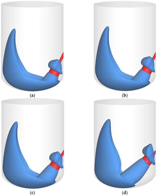
Figure 8.
The well-mixed volume of fluid in the tank with the inclination of the impeller equal to (a) 27°, (b) 30°, (c) 33°, (d) 45° for the case 1 impeller, which mixes ISR20.
The percentage of well-mixed liquid was calculated to determine how well the fluid was mixed. It was estimated as the fraction of the volume of the fluid with a velocity greater than 0.5 m/s to the volume of the entire system (Table 5). For each inclination, the percentage of well-mixed fluid is about 12%. However, the best mixing results are obtained with an inclination angle equal to 45°.
Table 5.
Comparison of percentage of well-mixed fluid and residence time for four values of impeller inclination for case 1, impeller mixing ISR20.
To ensure that the calculations were correct, the residence time was calculated. As mentioned, the flow rate was taken from Table 3 and is 0.525 m3/s, and the tank’s volume is 30 m3. The theoretical residence time (τ) can be determined using Equation (9).
The mean residence time was determined for each simulation by tracking the tracer introduced through the inlet to the tank. The results are shown in Table 5. The results show good convergence with the theoretical values.
3.2.2. The Dependence of the Mixing Ratio on the Type of Liquid
The results from the previous subsection suggest that the best results were obtained with an inclination angle equal to 45°. For this geometry, further calculations were performed. The effect of the type of fluid on the mixing ratio was investigated. As before, calculations were performed for the case 1 impeller; the flow rate for each fluid was taken from Table 3.
The mixing ratio was defined analogously to the previous subsection. The results are shown at Figure 9. The flow pattern for the jet flow mixer creates a circulation loop in the tank. For ISR20 and ISS, two of the most viscous liquids, the velocity of the fluid is high when the fluid exits the jet flow mixer. After a change in the flow direction caused by the wall, the liquid velocity drops below 0.5 m/s, resulting in a low mixing ratio of the fluid. There is a circulation loop with a zone in the middle of the tank for the other five liquids, where the fluid flow is almost unobserved. The strong dependence of the liquid flow in the upper part of the tank near the walls and underneath the mixer on viscosity was observed. The higher the viscosity, the larger the dead zones in the tank.
The fraction of well-mixed liquid was determined as described in the previous subsection. The results (Table 6) indicate that the mixing ratio is proportional to the decrease in the apparent viscosity of the fluid. The smallest mixing ratio (14.36%) was obtained for ISR20, whose viscosity is 5.48 Pa·s. The best mixing fluid is water, whose mixing ratio is almost 78%.
Table 6.
A comparison of the percentage of well-mixed fluid and the residence time for the six fluids (water, ISR20, ISR60, ISS, calcium carbonate suspension, and titanium dioxide suspension) in the tank with a jet flow mixer inclination angle equal to 45°.
The mean value of the residence time was determined (Table 6). The longest residence time was observed for ISR20, and the shortest for water. The residence time is connected to the flow rate of liquids, resulting in higher values for slower fluid flow. A good convergence of mean and theoretical residence time can be observed for all cases.
3.2.3. Power Consumption
Power consumption depends on the geometry and rotational speed of the mixer, power number (which is constant in turbulent flow for the considered agitator), and density. It was assumed that the density of ISR was the same as the density of water. These assumptions resulted in the same power consumption for these liquids. For the suspensions, power consumption increases with the concentration and properties of the suspended particles, resulting in the highest power consumption being for the calcium carbonate suspension.
The power consumption values were compared to shaft power values in (case 1) and are presented in Table 4. Relative errors were calculated and are presented in Table 7. The highest relative error values do not exceed 6% for the considered cases. Therefore, it can be assumed that simulations were conducted correctly.
Table 7.
Power consumption for six fluids in tank with jet flow mixer inclination angle equal to 45°.
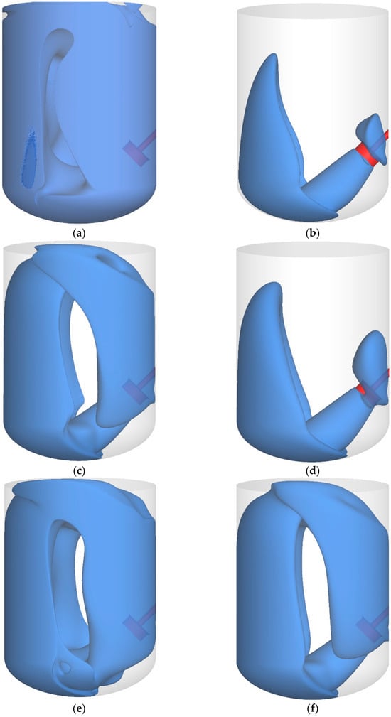
Figure 9.
The well-mixed volume of fluid in the tank with the inclination of the impeller equal to 45° for six types of fluid: (a) water, (b) industrially significant resin at 20 °C, (c) industrially significant resin at 60 °C, (d) industrially significant suspension, (e) calcium carbonate suspension, (f) titanium dioxide suspension.
4. Conclusions
In this study, the impact of the impeller’s geometry and the impeller’s positioning on mixing intensity was investigated. Calculations were performed in a real-size system, which resulted in obtaining real parameter values and, consequently, helped us to make well-informed industrial decisions. When performing CFD calculation, it is necessary to have literature or experimental data to validate the results. In this article, the obtained results were validated with literature data; however, performing experimental work would also be beneficial.
The result suggests that the propeller impeller with three blades (case 1) provides a good enough mixing quality while minimising power consumption. Calculations were performed for liquids with complex rheology, which resulted in a more comprehensive understanding of the fluid flow dynamics within the plant tank. Moreover, the optimal inclination angle for the impeller in a jet mixer is 45°. This configuration yields the most effective mixing quality. The intensity of the mixing process within the tank significantly depends on the fluids’ viscosity. The highest levels of mixing are achieved for the least viscous fluids. Nevertheless, the calculations demonstrated that the system under consideration requires a substantial power supply.
The results obtained indicate that the products within the tank are effectively mixed. In case of more viscous fluid, an additional mixer should be considered. Further calculations incorporating multiple jet flow mixers or additional mixers should be conducted in the future. The proposed methodology maximises mixing intensity for all fluid types, including Newtonian, non-Newtonian, and high-viscosity fluids, while reducing power consumption.
Author Contributions
Conceptualization and methodology, J.W., W.O., A.D. and Ł.M.; software, J.W. and Ł.M.; validation, J.W., P.G. and Ł.M.; formal analysis, W.O.; investigation, J.W.; writing—original draft preparation, J.W.; writing—review and editing, Ł.M., W.O., A.D. and P.G.; visualisation, J.W. and Ł.M.; supervision, Ł.M., P.G. and W.O.; project administration, W.O.; funding acquisition, W.O. and A.D. All authors have read and agreed to the published version of the manuscript.
Funding
This research was financially supported by hubergroup Polska sp. z o. o. Funding comes from the project entitled: ‘Development and demonstration of a modular, sustainable technology for the production of printing inks and varnishes using naturally derived components’, grant number FENG.01.01-IP.01-000L/23 given to hubergroup Polska sp. z o. o. by the National Centre for Research and Development. Julia Wilewska also acknowledges the financial support received from the IDUB project (Scholarship Plus programme).
Data Availability Statement
The original contributions presented in this study are included in the article. Further inquiries can be directed to the corresponding author.
Acknowledgments
This research was supported by hubergroup Polska sp. z o. o.
Conflicts of Interest
Author Adam Dudała was employed by the company hubergroup Polska Sp. Z o.o. The remaining authors declare that the research was conducted in the absence of any commercial or financial relationships that could be construed as a potential conflict of interest.
References
- Kelly, W.; Gigas, B. Using CFD to Predict the Behavior of Power Law Fluids near Axial-Flow Impellers Operating in the Transitional Flow Regime. Chem. Eng. Sci. 2003, 58, 2141–2152. [Google Scholar] [CrossRef]
- Dakshinamoorthy, D.; Khopkar, A.R.; Louvar, J.F.; Ranade, V.V. CFD Simulation of Shortstopping Runaway Reactions in Vessels Agitated with Impellers and Jets. J. Loss Prev. Process Ind. 2006, 19, 570–581. [Google Scholar] [CrossRef]
- Wang, P.; Reviol, T.; Kluck, S.; Würtz, P.; Böhle, M. Mixing of Non-Newtonian Fluids in a Cylindrical Stirred Vessel Equipped with a Novel Side-Entry Propeller. Chem. Eng. Sci. 2018, 190, 384–395. [Google Scholar] [CrossRef]
- Paul, E.L.; Atiemo-Obeng, V.A.; Kresta, S.M. Handbook of Industrial Mixing: Science and Practice; American Institute of Chemical Engineers, Ed.; Wiley-Interscience: Hoboken, NJ, USA, 2004; ISBN 978-0-471-26919-9. [Google Scholar]
- Hall, S. Blending and Agitation. In Branan’s Rules of Thumb for Chemical Engineers; Elsevier: Amsterdam, The Netherlands, 2012; pp. 257–279. ISBN 978-0-12-387785-7. [Google Scholar]
- Stelmach, J.; Kuncewicz, C.; Jirout, T.; Rieger, F. Mixing Tank Hydrodynamics and Mixing Efficiency for Propeller Impellers. Chem. Eng. Res. Des. 2023, 199, 460–472. [Google Scholar] [CrossRef]
- Madhania, S.; Fathonah, N.N.; Kusdianto; Nurtono, T.; Winardi, S. Turbulence Modeling in Side-Entry Stirred Tank Mixing Time Determination. MATEC Web Conf. 2021, 333, 02003. [Google Scholar] [CrossRef]
- Madhania, S.; Nurtono, T.; Cahyani, A.B.; Carolina; Muharam, Y.; Winardi, S.; Purwanto, W.W. Mixing Behaviour of Miscible Liquid-Liquid Multiphase Flow in Stirred Tank with Different Marine Propeller Installment by Computational Fluid Dynamics Method. Chem. Eng. Trans. 2017, 56, 1057–1062. [Google Scholar] [CrossRef]
- Ge, C.-Y.; Wang, J.-J.; Gu, X.-P.; Feng, L.-F. CFD Simulation and PIV Measurement of the Flow Field Generated by Modified Pitched Blade Turbine Impellers. Chem. Eng. Res. Des. 2014, 92, 1027–1036. [Google Scholar] [CrossRef]
- Havas, G.; Deak, A.; Fekete, A. Investigation of the Homogenization Efficiency of Various Propeller Agitator Types. Period. Polytech. Chem. Eng. 1978, 22, 331–334. [Google Scholar]
- Stoops, C.E.; Lovell, C.L. Power Consumption of Propeller-Type Agitators. Ind. Eng. Chem. 1943, 35, 845–850. [Google Scholar] [CrossRef]
- Pukkella, A.K.; Vysyaraju, R.; Tammishetti, V.; Rai, B.; Subramanian, S. Improved Mixing of Solid Suspensions in Stirred Tanks with Interface Baffles: CFD Simulation and Experimental Validation. Chem. Eng. J. 2019, 358, 621–633. [Google Scholar] [CrossRef]
- Kresta, S.M.; Etchells, A.W.; Dickey, D.S.; Atiemo-Obeng, V.A. Advances in Industrial Mixing: A Companion to the Handbook of Industrial Mixing; American Institute of Chemical Engineers, Ed.; Wiley: Hoboken, NJ, USA, 2016; ISBN 978-0-470-52382-7. [Google Scholar]
- Metzner, A.B.; Otto, R.E. Agitation of non-Newtonian Fluids. AIChE J. 1957, 3, 3–10. [Google Scholar] [CrossRef]
- Wang, S.; Wang, P.; Yuan, J.; Liu, J.; Si, Q.; Li, D. Simulation Analysis of Power Consumption and Mixing Time of Pseudoplastic Non-Newtonian Fluids with a Propeller Agitator. Energies 2022, 15, 4561. [Google Scholar] [CrossRef]
- Bumrungthaichaichan, E.; Wattananusorn, S. CFD Modelling of Pump-around Jet Mixing Tanks: A Reliable Model for Overall Mixing Time Prediction. J. Chin. Inst. Eng. 2019, 42, 428–437. [Google Scholar] [CrossRef]
- Patwardhan, A.W.; Gaikwad, S.G. Mixing in Tanks Agitated by Jets. Chem. Eng. Res. Des. 2003, 81, 211–220. [Google Scholar] [CrossRef]
- Zughbi, H.D.; Rakib, M.A. Mixing in a Fluid Jet Agitated Tank: Effects of Jet Angle and Elevation and Number of Jets. Chem. Eng. Sci. 2004, 59, 829–842. [Google Scholar] [CrossRef]
- Grenville, R.K.; Tilton, J.N. Jet Mixing in Tall Tanks: Comparison of Methods for Predicting Blend Times. Chem. Eng. Res. Des. 2011, 89, 2501–2506. [Google Scholar] [CrossRef]
- Jayanti, S. Hydrodynamics of Jet Mixing in Vessels. Chem. Eng. Sci. 2001, 56, 193–210. [Google Scholar] [CrossRef]
- Manjula, P.; Kalaichelvi, P.; Dheenathayalan, K. Development of Mixing Time Correlation for a Double Jet Mixer. J. Chem. Technol. Biotechnol. 2010, 85, 115–120. [Google Scholar] [CrossRef]
- Rahimi, M.; Parvareh, A. CFD Study on Mixing by Coupled Jet-Impeller Mixers in a Large Crude Oil Storage Tank. Comput. Chem. Eng. 2007, 31, 737–744. [Google Scholar] [CrossRef]
- Karbstein, H.; Schubert, H. Developments in the Continuous Mechanical Production of Oil-in-Water Macro-Emulsions. Chem. Eng. Process. Process Intensif. 1995, 34, 205–211. [Google Scholar] [CrossRef]
- Atiemo-Obeng, V.A.; Penney, W.R.; Armenante, P. Solid–Liquid Mixing. In Handbook of Industrial Mixing; Paul, E.L., Atiemo-Obeng, V.A., Kresta, S.M., Eds.; Wiley: Hoboken, NJ, USA, 2003; pp. 543–584. ISBN 978-0-471-26919-9. [Google Scholar]
- Zhang, J.; Xu, S.; Li, W. High Shear Mixers: A Review of Typical Applications and Studies on Power Draw, Flow Pattern, Energy Dissipation and Transfer Properties. Chem. Eng. Process. Process Intensif. 2012, 57–58, 25–41. [Google Scholar] [CrossRef]
- Vashisth, V.; Nigam, K.D.P.; Kumar, V. Design and Development of High Shear Mixers: Fundamentals, Applications and Recent Progress. Chem. Eng. Sci. 2021, 232, 116296. [Google Scholar] [CrossRef]
- Håkansson, A. The Dissipation Rate of Turbulent Kinetic Energy and Its Relation to Pumping Power in Inline Rotor-Stator Mixers. Chem. Eng. Process. Process Intensif. 2017, 115, 46–55. [Google Scholar] [CrossRef]
- Xu, S.; Cheng, Q.; Li, W.; Zhang, J. LDA Measurements and CFD Simulations of an In-Line High Shear Mixer with Ultrafine Teeth. AIChE J. 2014, 60, 1143–1155. [Google Scholar] [CrossRef]
- Pacek, A.; Baker, M.; Utomo, A.T. Characterisation of Flow Pattern in a Rotor Stator High Shear Mixer. In Proceedings of the European Congress of Chemical Engineering (ECCE-6), Copenhagen, Denmark, 16–20 September 2007. [Google Scholar]
- Mortensen, H.H.; Arlov, D.; Innings, F.; Håkansson, A. A Validation of Commonly Used CFD Methods Applied to Rotor Stator Mixers Using PIV Measurements of Fluid Velocity and Turbulence. Chem. Eng. Sci. 2018, 177, 340–353. [Google Scholar] [CrossRef]
- Mortensen, H.H.; Calabrese, R.V.; Innings, F.; Rosendahl, L. Characteristics of Batch Rotor–Stator Mixer Performance Elucidated by Shaft Torque and Angle Resolved PIV Measurements. Can. J. Chem. Eng. 2011, 89, 1076–1095. [Google Scholar] [CrossRef]
- Wu, H.; Shu, S.; Yang, N.; Lian, G.; Zhu, S.; Liu, M. Modeling of Power Characteristics for Multistage Rotor–Stator Mixers of Shear-Thinning Fluids. Chem. Eng. Sci. 2014, 117, 173–182. [Google Scholar] [CrossRef]
- Jasińska, M.; Bałdyga, J.; Cooke, M.; Kowalski, A.J. Specific Features of Power Characteristics of In-Line Rotor–Stator Mixers. Chem. Eng. Process. Process Intensif. 2015, 91, 43–56. [Google Scholar] [CrossRef]
- Özcan-Taşkın, G.; Kubicki, D.; Padron, G. Power and Flow Characteristics of Three Rotor-stator Heads. Can. J. Chem. Eng. 2011, 89, 1005–1017. [Google Scholar] [CrossRef]
- Xu, S.; Shi, J.; Cheng, Q.; Li, W.; Zhang, J. Residence Time Distributions of In-Line High Shear Mixers with Ultrafine Teeth. Chem. Eng. Sci. 2013, 87, 111–121. [Google Scholar] [CrossRef]
- Wasewar, K.L. A Design of Jet Mixed Tank. Chem. Biochem. Eng. Q. 2006, 20, 31–46. [Google Scholar]
- Wang, P.; Reviol, T.; Ren, H.; Böhle, M. Effects of Turbulence Modeling on the Prediction of Flow Characteristics of Mixing Non-Newtonian Fluids in a Stirred Vessel. Chem. Eng. Res. Des. 2019, 147, 259–277. [Google Scholar] [CrossRef]
- Haque, J.N.; Mahmud, T.; Roberts, K.J.; Rhodes, D. Modeling Turbulent Flows with Free-Surface in Unbaffled Agitated Vessels. Ind. Eng. Chem. Res. 2006, 45, 2881–2891. [Google Scholar] [CrossRef]
- Shi, J.; Zhao, Z.; Song, W.; Jin, Y.; Lu, J. Numerical Simulation Analysis of Flow Characteristics in the Cavity of the Rotor-Stator System. Eng. Appl. Comput. Fluid Mech. 2022, 16, 501–513. [Google Scholar] [CrossRef]
- Luo, J.Y.; Issa, R.I.; Gosman, A.D. Prediction of Impeller Induced Flows in Mixing Vessels Using Multiple Frames of Reference. IChemE Symp. Ser. 1994, 136, 549–556. [Google Scholar]
- Wallin, S.; Johansson, A. Fluent Theory Guide. 2025. Available online: https://ansyshelp.ansys.com/public/account/secured?returnurl=/Views/Secured/prod_page.html?pn=Fluent (accessed on 17 July 2025).
- Patil, H.; Patel, A.K.; Pant, H.J.; Venu Vinod, A. CFD Simulation Model for Mixing Tank Using Multiple Reference Frame (MRF) Impeller Rotation. ISH J. Hydraul. Eng. 2021, 27, 200–209. [Google Scholar] [CrossRef]
- John, T.P.; Fonte, C.P.; Kowalski, A.; Rodgers, T.L. A Comparison of Power and Flow Characteristics between Batch and In-Line Rotor-Stator Mixers. Chem. Eng. Sci. 2019, 202, 481–490. [Google Scholar] [CrossRef]
- Wang, J.; Huang, Y.; Zhang, R.; Zhou, L. Numerical and Experimental Study of Homogenization Mechanism of High Shear Rotor-stator Mixer. Can. J. Chem. Eng. 2024, 102, 4216–4229. [Google Scholar] [CrossRef]
- Kugge, C.; Daicic, J. Shear Response of Concentrated Calcium Carbonate Suspensions. J. Colloid Interface Sci. 2004, 271, 241–248. [Google Scholar] [CrossRef] [PubMed]
- Bingham, E.C. Fluidity and Plasticity; Mcgraw-Hill Book Company: New York, NY, USA, 1922. [Google Scholar]
- Krzosa, R.; Makowski, Ł.; Orciuch, W.; Adamek, R. Population Balance Application in TiO2 Particle Deagglomeration Process Modeling. Energies 2021, 14, 3523. [Google Scholar] [CrossRef]
- Carreau, P.J. Rheological Equations from Molecular Network Theories. Trans. Soc. Rheol. 1972, 16, 99–127. [Google Scholar] [CrossRef]
- Jain, M.; Misumi, R. Experimental Investigation of the Power Consumption and Metzner–Otto Constant for Highly Shear-Thinning Fluids with Different Impeller Geometries. J. Chem. Eng. Jpn. 2024, 57, 2387459. [Google Scholar] [CrossRef]
- Nagata, S.; Yamamoto, K.; Yokoyama, T.; Shiga, S. Studies on the Power Requirement of Mixing Impellers (IV): Empirical Equations Applicable for a Wide Range. Mem. Fac. Eng. Kyoto Univ. 1957, 19, 274–289. [Google Scholar]
- Nagata, S. Mixing—Principles and Applications; Halsted Press: Sydney, NSW, Australia, 1976; p. 22. [Google Scholar] [CrossRef]
Disclaimer/Publisher’s Note: The statements, opinions and data contained in all publications are solely those of the individual author(s) and contributor(s) and not of MDPI and/or the editor(s). MDPI and/or the editor(s) disclaim responsibility for any injury to people or property resulting from any ideas, methods, instructions or products referred to in the content. |
© 2025 by the authors. Licensee MDPI, Basel, Switzerland. This article is an open access article distributed under the terms and conditions of the Creative Commons Attribution (CC BY) license (https://creativecommons.org/licenses/by/4.0/).