Abstract
Understanding the dynamic carbon emission status is vital for turning a power system into a low-carbon system. However, the existing research has normally considered the average carbon emissions as the indicator for the operation and planning of power systems. Detailed carbon emission responsibility is not well allocated to different demands within power systems, leading to inefficient emission control. To address this problem, this paper develops a data-driven method for accurately finding the characteristics of the nodal marginal emission factor without the requirement of real-time optimal power flow (OPF) simulation. First, the nodal marginal emission factor system is derived based on actual data covering a timespan of one year on top of the IEEE 118 system. Then, a Graphical Neural Network (GNN) is adopted to map both the spatial and temporal relationship between nodal marginal emission and other features, thereby identifying the marginal emission characteristics for different nodes of power transmission systems. Through case studies, fine-tuned GNNs estimate all nodal marginal emission factor (NMEF) values for power systems without the requirement of OPF simulation and achieve a 5.75% Normalized Root Mean Squared Error (nRMSE) and 2.52% Normalized Mean Absolute Error (nMAE). Last but not least, this paper brings a new finding: a strong inclination to reduce marginal emission rates would compromise economic operation for power systems.
1. Introduction
Since 2010, average carbon emissions (ACEs) from the U.S. electric power sector have fallen by 28% while a 7% increase in marginal emissions has been found during the same period [1]. This counterintuitive scenario has raised an industry request: real-time marginal carbon emission monitoring, particularly for each node of power systems, is also vital in ensuring an efficient low-carbon transformation of power systems. Compared to the traditional carbon emission factor, measuring the marginal carbon emission is a solution to achieve carbon emission monitoring [2]. However, the characteristics of nodal marginal emission within power transmission systems remain unknown, particularly with significant violations of renewable generation in power transmission systems. The uncertainty of load and renewable energy generation [3] further complicates the accurate observation of nodal marginal emissions.
Currently, power system classically adopts ACE measurement, also named as the carbon emission factor [4]. The carbon emission factor method is a method proposed by the Intergovernmental Panel on Climate Change (IPCC). It refers to the activity intensity data collected throughout the entire life cycle of electricity, from production to installation, maintenance, and finally recycling [5]. Reference [6] calculated carbon emission factors by disaggregating hourly electricity generation data (2016–2017) by energy sources (fossil fuels and renewables) in Italy, defining three dynamic CO2 emission indicators to quantify the carbon intensity per kWh under varying generation mixes. Reference [7] developed a piecewise nonlinear unit-level dynamic emission factor (P-UDEF) model that accurately estimates real-time carbon emission factors by fitting actual operational data (e.g., during startup and steady-state phases) through segmented parametric regression. Reference [8] adopted a life-cycle assessment (LCA) framework to quantify the carbon emissions attributable to the United Kingdom’s transmission network over a 40-year service life on this foundation. The results compared the ratio of carbon emissions from grid operations to those from raw materials themselves. Reference [9] used this method to evaluate Norway’s distribution network. The results compared the contribution of transmission grids and distribution grids to carbon emissions. To evaluate the configuration of power grid assets, reference [10] compared the carbon emissions over the life cycle of ultra-high voltage direct current (UHVDC) transmission facilities with the carbon emission reductions achieved by these facilities using this method. Reference [11] studied the allocation of carbon emission quotas among provinces in China, with the main research objective being to understand the total carbon emissions from thermal power generation among provinces. Although the carbon emission factor is classic, easy-to-understand, and generally applied, it still has limitations in quantifying the carbon emissions by the action of different demands. This leads to difficulty in recognizing the shares of responsibility of different demands in the total carbon emissions of power systems.
To address the limitation of the carbon emission factor, the carbon emission flow has been developed. The concept of carbon emission flow uses virtual carbon emissions to simulate the transfer process of carbon emissions. Given the power flow, the virtual carbon emissions corresponding to each megawatt hour of electricity can be calculated to label the carbon emissions of the transmitted electricity. A distributed algorithm based on matrix partitioning and parallel computing was developed in [12], where it distributed the calculation of CEF across multiple terminals. This method significantly improved the efficiency of large-scale grid carbon emission calculations. Reference [13] developed a CEF model that surpasses conventional macro-statistical and LCA approaches, enabling the precise tracking of carbon footprints during power transmission and use. Reference [14] proposed a new CEF model under multiple energy systems to quantify carbon emissions related to energy transport and conversion processes. Reference [15] developed an improved CEF method that integrates graph theory and power flow tracing to quantify the impact of prosumers on grid carbon emissions while developing a dynamic carbon emission intensity model accounting for distributed energy resources and energy storage systems. Reference [16] applied CEF to establish a demand-side management model for electricity and carbon emission trading markets based on carbon emission flows. While the carbon emission flow (CEF) method effectively characterizes the spatial redistribution of emissions across power networks, its practical application is constrained by two fundamental limitations: (1) computational complexity that scales exponentially with system node count and (2) an inherent inability to quantify the marginal emission impact of incremental electricity demand. These limitations restrict its utility for real-time operational dispatch and carbon-aware electricity pricing mechanisms.
Towards the objective evaluation of the accuracy of marginal emissions factors, the existing research has typically employed calculation methods centered on real-world data and the operational mechanisms of power generation units. Real-world data is generally obtained using the post-measurement method over a full year. Reference [17] applied this method to quantify the impact of renewable energy deployment on European Union Allowance prices and carbon dioxide emissions in the power sectors of Western and Southern Europe from 2007 to 2010. Reference [18] performed regression analysis on U.S. electricity generation and emissions data from 2006 to 2011 to estimate marginal carbon emissions in the continental United States. However, due to their simplicity, these methods do not account for power system topology constraints, limiting their ability to accurately quantify the real-time responses of different demand nodes to system emissions. This approach dilutes the impact of specific regions or units within the system on the entire power system.
An improved approach focuses on a computational method based on power plant dispatch mechanisms. These methods estimate the cost of each power plant (including fuel, variable operating costs, and maintenance costs). The plants are ranked in ascending order of cost and assumed to be dispatched in sequence until the total supply equals the simulated demand value [19]. However, such methods ignore issues related to transmission. At the sub-regional level, the model assumes that transmission capacity is unlimited. It also ignores wind power curtailment and solar power curtailment. This may affect the accuracy of the simulated marginal emission [20]. It proposes to quantify the changes in emissions caused by changes in the demand of power system nodes and map them to marginal electricity prices to bridge the gap between macro-level results and the inability to conduct a detailed assessment of local marginal carbon emissions. Reference [21] employs implicit differentiation via a single inversion of the OPF’s KKT Jacobian to compute marginal emissions. In practical OPF formulations, however, discrete unit-commitment decisions, ramp-rate constraints, and piecewise emission functions violate the requisite smoothness. Consequently, the method often exhibits numerical instability or fails on detailed system models. Compared to existing marginal emission factor methodologies, the developed OPF method in this study accounts for inter-nodal propagation and improves the accuracy of the prediction when the penetration of new energy sources increases. However, for large-scale systems with increased complexity, the simulation results take significantly longer to generate [22]. Processing these results without using a learning model is time-consuming and resource-intensive [23].
Given the aforementioned problems for both marginal and average emission factoring methods, a gap exists between carbon measurement in power systems and the real-time operation of power systems: it require an accurate and effective carbon measurement method to characterize the spatiotemporal heterogeneity of regional and temporal carbon emissions and provide in-depth guidance for the low-carbon operation of power systems.
To bridge this gap, this paper develops a data-driven method for accurately finding the characteristics of the nodal marginal emission factor without the requirement of real-time OPF simulation. First, the nodal marginal emission factor system is derived based on actual data covering a timespan of one year. Direct-current OPF is adopted to simulate the power system dispatching strategies, where a cost-weighted carbon-emission objective is specifically designed. Then, the derived time-series nodal marginal emissions are restructured with time-series demand, renewable generations, and environment features (such as temperature, humidity, wind speed, etc.). Finally, the Graphical Neural Network (GNN) is adopted to learn the spatial and temporal relationship between nodal marginal emission and other features, thereby identifying the marginal emission characteristics for different nodes of power transmission systems. Given the trained GNN model, the power system engineers could fast estimate nodal marginal emission rates (also called factors) without the requirement for tuning and operating the time-consuming OPF model.
This paper brings the following original contributions:
- (1)
- This paper originally identifies the marginal emission characteristics for different nodes of power transmission systems considering power-system operational constraints.
- (2)
- In application, field engineers do not need to understand and tune the complex optimal power flow model. Light training on data organization could support engineers in estimating nodal marginal emission rates (also called factors).
2. Methodology
2.1. Overview of the Methodology
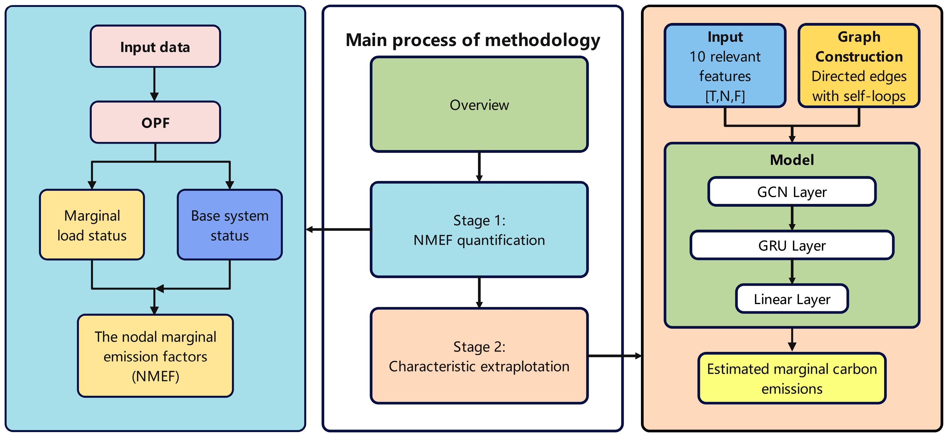
This section overviews the methodology of this paper, commencing from the measurement of nodal marginal emission factor (NMEF) to dataset organization and concluding with the extrapolation of NMEF characteristics. The flowchart of the methodology is shown in Figure 1.
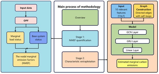
Figure 1.
The flowchart of the developed methodology.
In stage 1, the model for deriving NMEF is developed. Compared to traditional emission factor measurement on average, NMEF indicates the emission difference between the current system emission and the marginal system emission. The marginal system emission refers to the emission caused by 1-unit power increment in a given nodal. Therefore, NMEF could be a positive value for a load node and a negative value for a generation node. The following is a simplified example for NMEF. If the demand of one node is 100 MW throughout one hour and the system carbon emission from all power plants is 80 tons, by increasing the demand of this given nodal from 100 to 101 MW, the system carbon emission changes to 80.9 tons. The NMEF is (80.9–80)/1 MW, which equals 0.9 tons/MWh. It is clearly seen that the NMEF is highly related to the system operation change with 1 MW power increase for the given nodal. To obtain the ex-post system operation status, this paper adopts direct-current (DC) optimal power flow (OPF) to simulate the dispatching strategies of generations. By comparing the emission ex ante and ex post, NMEF is derived.
Stage 2 aims to find the characteristics of NMEF. The derived characteristic model could directly estimate NMEF without the requirement of carrying out time- and resource-consuming OPF in real time. To this end, this stage develops a spatiotemporal deep learning model to estimate the NMEF based on historical operation data. The input to the model is a set of node feature tensors for 24 consecutive hours, and the features include 10 metrics such as load, voltage phase angle, and power generation at each node. The model first spatially models each time step using a graph convolutional layer (GCN) to capture the information flow and interactions between neighboring nodes in the grid graph structure. Subsequently, the graph convolution outputs of all time steps are concatenated into a time series on a node-by-node basis and fed into a gated recurrent unit (GRU) to model the temporal dependencies, which, in turn, extracts the dynamic operating modes of each node. The training objective is to minimize the Normalized Root Mean Squared Error (nRMSE) between the estimated values and the true NMEF values obtained through the OPF method in the first stage so that the model can effectively learn the nonlinear mapping relationship between the marginal emissions of the system and the historical operating states.
Once training is completed, the GNN model can be used to make estimations of marginal carbon emissions for future periods. This stage realizes the transformation of marginal carbon emissions from physical-simulation-based to data-driven intelligent modeling and lays the algorithmic foundation for real-time carbon emission monitoring and low-carbon scheduling strategies.
2.2. Measurement of Nodal Marginal Emission Factors
This section details the methodology of deriving NMEF. The first step derives the system’s base carbon emissions on top of the original input data. Second, the method for deriving system carbon emissions under marginal demand and marginal renewable generation status is developed. Third, by comparing system base carbon emissions with ex post system emissions under marginal status, the NMEFs for both the demand node and renewable node are derived.
2.2.1. Deriving the Base-System Carbon Emissions
This section adopts the DC OPF to derive the dispatching strategies of generators, alongside the base system carbon emissions, before deriving NMEF.
First, given the time step , the objective function of the DC OPF is defined as given below:
Here, is the output power of the solar power station at time ; is the output power of the wind farm at time ; is the output power of the gas generator at time ; is the output power of the coal generator at time ; and are fuel price weights aligned to carbon emissions from coal and gas generators, respectively; represents the carbon emission from the coal generator at time ; are weights for the carbon emission function for the coal generator; represents the carbon emission from the gas generator at time t; are weights for the carbon emission function for the gas generator.
The objective function of Equation (1) means minimizing the weight carbon emissions from both gas and coal generators. The reason for assigning the fuel price weight is considering both generation costs and price, thus preventing the dispatching strategies over inclines to gas generators with lower emission factors.
With the developed objective function, the constraints for solving the DC OPF are given as follows.
The power balance constraint is given below:
Here, are the output power variables for the solar power stations, wind farms, and gas and coal generators connected to the node at time , respectively; is demand power connected to the node at time ; represents the power flows from node to its connected node at time .
The power constraint of each line is given below:
Here, is the phase angle of node at time ; is the phase angle of node at time ; is the reactance of the transmission line between node and .
The capacity constraint of each line is given below:
Here, is the maximum capacity of the transmission line between node and .
The power constraints for solar power stations, wind farms, and gas and coal generators are given below:
Here, and are the minimum and maximum output power of the solar power station at time , respectively; is the output power of the solar power station at time ; and are the minimum and maximum output power of the wind farm at time , respectively; is the output power of the wind farm at time ; and are the minimum and maximum output power of the gas generator at time , respectively; is the output power of the gas generator at time ; and are the minimum and maximum output power of the coal generator at time , respectively; is the output power of the coal generator at time ; , , , are defined as the actual power variables at time at respective nodes.
It should be noted that in Equations (7) and (8), the minimal and maximum power for solar power stations and wind farms are changing. This setting reflects the reality, where the theoretical maximum power are determined by the real-time solar radiation and wind speed.
Further, the phase angle constraint is given below:
Here, is the phase angle of node at time . The phase angle of the reference node is set to 0:
By solving the aforementioned DC OPF problem, the base system carbon emission is given below:
Here, and are defined in Equations (2) and (3).
2.2.2. Deriving the System Carbon Emissions Under Marginal Load Status
This section presents the process for deriving the system carbon emissions under marginal load status. Taking the demand node at the time step as the example, the process is shown as follows:
Given the same input data as those in Section 2.2.1:
For demand node , we increase the load power by 1 MW as given below:
We replace with and keep other data constant.
We solve the optimal power flow problem in Section 2.2.1 and derive the system carbon emissions under the marginal load scenarios for the demand node.
To derive the system carbon emissions under the marginal load scenarios for all demand node, the above 4 steps would be repeatedly applied regarding from first demand node to the last demand node.
2.2.3. Deriving the Nodal Marginal Emission Factor
With the obtained base system carbon emission , the system carbon emissions under marginal load status , and the system carbon emissions under marginal renewable generation status , the nodal marginal emission factors for the demand node and the renewable node are given below:
2.3. Data-Driven Modeling of the Characteristics of Marginal CO2 Emissions Using Temporal Graph Neural Networks
Following the derivation of nodal marginal emission factors (NMEFs) via optimal power flow (OPF) simulations in the first stage, the second stage of the methodology focuses on constructing a data-driven learning framework to extrapolate the characteristics of NMEF at each node in the power system. To capture both the spatial dependencies inherent in power network topology as well as temporal correlations within operational features, GNN architecture is proposed. This model integrates graph convolutional layers for spatial feature extraction and GRU for sequential modeling.
2.3.1. Input Representation and Data Preparation
The input to the model is structured as a spatiotemporal tensor of shape [T,N,F], where T = 24 is the time window length (i.e., the number of historical hours used), N denotes the number of nodes in the system (118 in this study), and F represents the number of input features per node. The features include the following: load demand, voltage angle, generator output, node-level carbon emissions, renewable generation (wind and solar), generator type, system-level carbon indicators (total and average emissions), and total power generation.
The temporal dataset is first standardized using a StandardScaler and then converted into a sliding-window format to form supervised samples for training. For each 24 h window, the target is the corresponding NMEF value for each node at the next hour, as computed in the first stage via OPF-based simulations.
2.3.2. Graph Construction
In order to capture the spatial topology of the grid, a directed graph is constructed based on the directional links between buses, as shown in Figure 2. Each node corresponds to a bus in the IEEE 118 bus system, each edge represents the directional link between the two buses, and the direction of the edge arrow indicates the direction of power transfer. To ensure stability during training and avoid isolated nodes, self-loops (blue arcs) are added to all nodes.
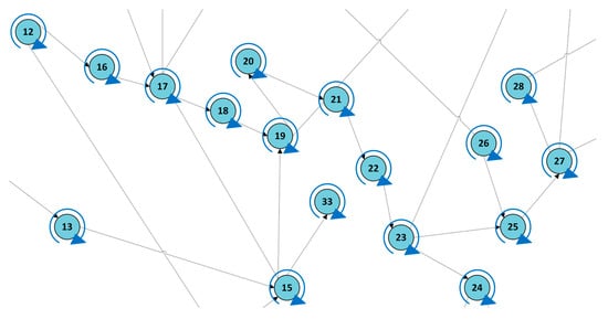
Figure 2.
Graph of 118 nodes with edges.
Based on the topology, the adjacent matrix of the nodes is further constructed for explicitly representing the connectivity between the nodes; the adjacency matrix is defined as follows:
Here, each element indicates the connection between node and node :
The matrix A describes the connectivity between the nodes, where the rows and columns correspond to 118 nodes. The matrix element indicates the existence of a directed transmission link from node i to node j. The main diagonal (red) indicates the node self-loop. This matrix is used as input to the graph convolutional layers of the model.
2.3.3. Model Architecture
To capture the spatial dependencies inherent in graph-structured data, we employ the GCN. Unlike traditional convolutional neural networks designed for grid-like Euclidean data, GCNs generalize convolution operations to irregular graph domains by aggregating feature information from neighboring nodes.
Given a graph with node set and edge set , and the corresponding adjacency matrix ∈ , where , the graph convolution operation for one layer is defined thus:
Here, is the adjacency matrix with added self-connections, is the diagonal degree matrix of , is the input feature matrix at layer , is the learnable weight matrix of layer , and is a nonlinear activation function such as ReLU.
This operation effectively propagates and transforms node features by aggregating information from immediate neighbors, enabling the model to learn representations that encode spatial relationships in the graph.
To model temporal dependencies in sequential data, we integrate a Gated Recurrent Unit (GRU) network. GRUs constitute a type of recurrent neural network that efficiently capture long-range temporal dependencies by employing gating mechanisms to control information flow, mitigating the vanishing gradient problem common in traditional RNNs. The core components of the GRU are the update gate and the reset gate. The role of the update gate is to determine how much information from the previous time step needs to be retained for the hidden state of the current time step. The update gate is given below:
Here, and are the parameter matrices and bias vectors of the update gate, is the previous time step’s hidden state, and is the current input.
The reset gate determines to what extent the hidden state of the previous time step is ignored. The formula for the reset gate is given below:
Here, and are the parameter matrices and bias vectors of the reset gate.
2.3.4. Training and Evaluation
The model is trained in a supervised fashion using the mean squared error (MSE) loss between the estimated and true NMEF values:
Here, is the batch size. The Adam optimizer is used with a learning rate of 0.001. The dataset is partitioned chronologically into training (70%), validation (15%), and testing (15%) sets. To evaluate the model’s performance, the root mean square error (RMSE) and Normalized Mean Absolute Error (nMAE) are computed on the test set. Furthermore, visualization techniques are employed to plot the estimated versus actual NMEF values and to examine temporal estimation patterns at selected nodes.
3. Case Studies
This section presents the simulation results. The input data are given in Section 3.1. The quantification of marginal carbon emissions is shown in Section 3.2. The characteristics of NMEF are presented in Section 3.3. And Section 3.4 discusses the outcome of this case.
3.1. Input Data
This paper adopts the IEEE 118 buses template as the testing system [24]. The testing system comprises 27 generators and 186 branches. Inside the system, 99 nodes are connected to demand. The generator components of this system have been modified to match current conditions into four types: coal generators, gas generators, wind farms, and solar power stations. The maximum power outputs, locations, and types of different generators are shown in Table 1 [25]. The fuel consumption curve equations for coal generators and gas generators with different maximum power outputs are shown in Table 2 [26,27,28]. According to the differences in fuel costs between coal generators and gas generators, the fuel price weight aligned to carbon emissions from gas generators is set to 3. The fuel price weights aligned to carbon emissions from coal generators is set to 1. For real-time data, the time-series output from wind farms and solar power stations are estimated based on wind speed and solar irradiance from Hainan Province’s 2023 meteorological data. The time series demand for each node was extracted from the Australia open dataset throughout 2023 [29].

Table 1.
Detailed parameters of each unit of the generator.
Table 2.
Fuel consumption curve of traditional energy generators.
3.2. Quantification of Marginal Carbon Emission Simulation
By simulating the IEEE 118 system with the developed methodology in Section 2.2, this section gives the results of NMEF quantification and provides a spatiotemporal comparison between ACE and NMEF on typical days. Figure 3 depicts the derived NMEF for all 118 nodes throughout 24 h, where carbon-sensitive nodes and critical periods are identified. Figure 4 compares ACE and NMEF for all nodes at four representative hours (5 h, 13 h, 16 h, and 19 h). Figure 5 details the variation of ACE and NMEF for five representative nodes throughout 24 h.

Figure 3.
Heatmap of NMEF on 6 July.
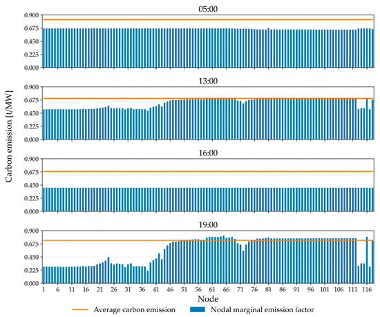
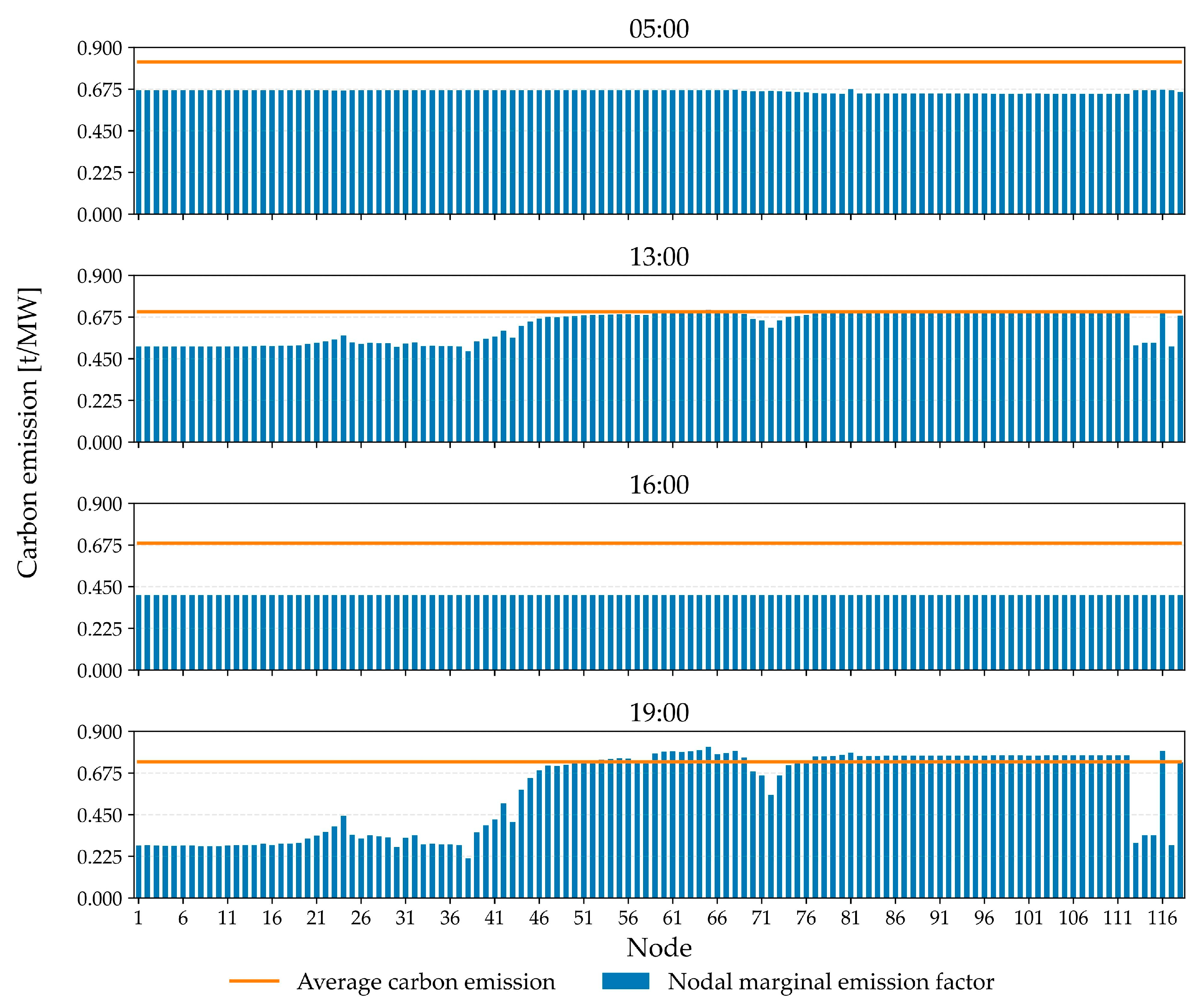
Figure 4.
Comparison of NMEF and ACE in four representative time periods.
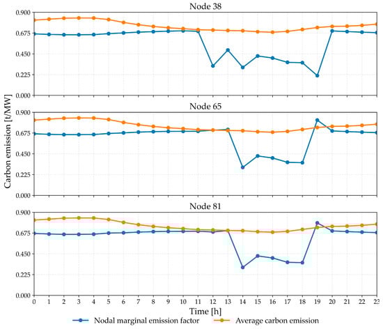
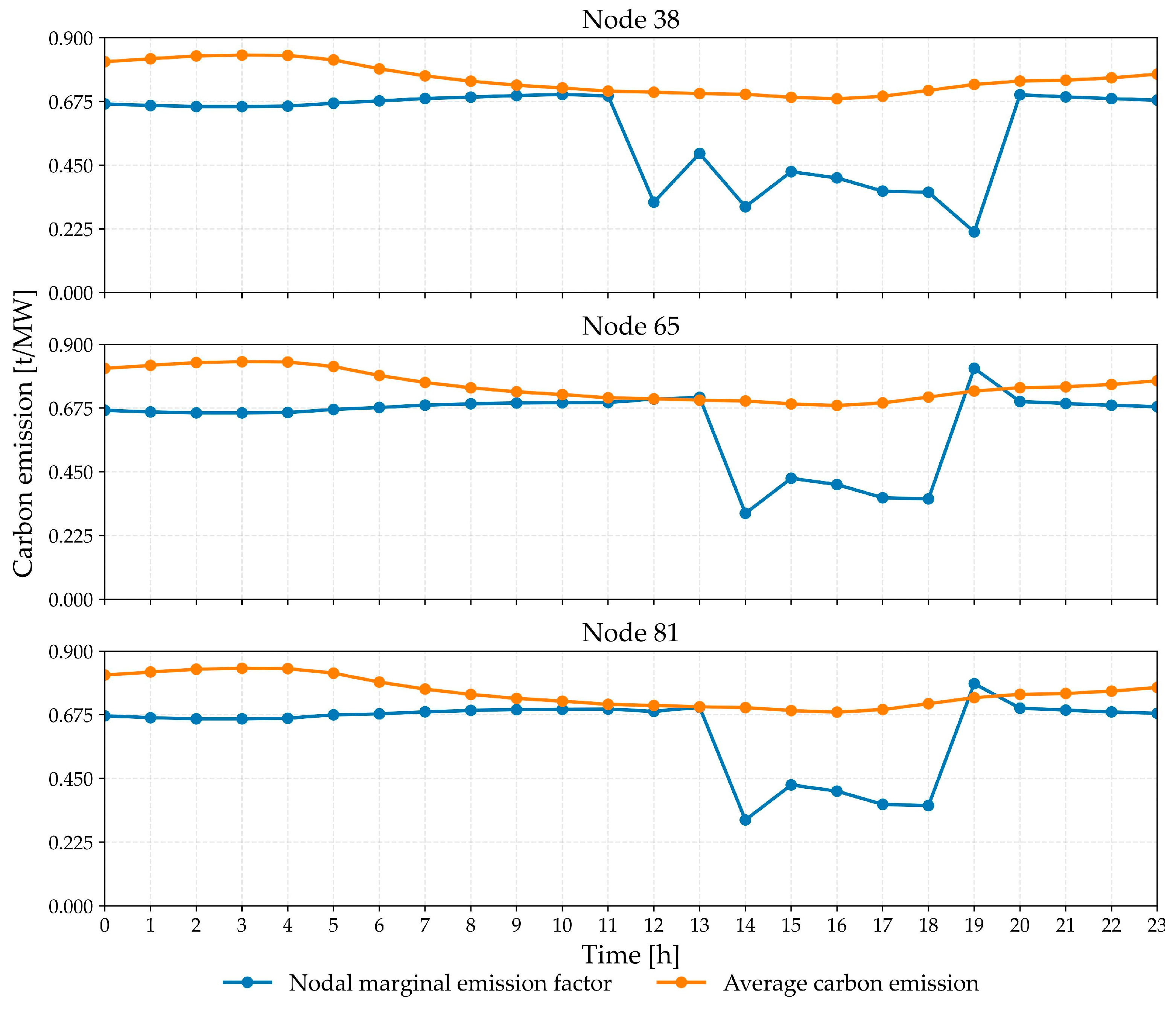
Figure 5.
Comparison of NMEF and ACE in five typical nodes is identified.
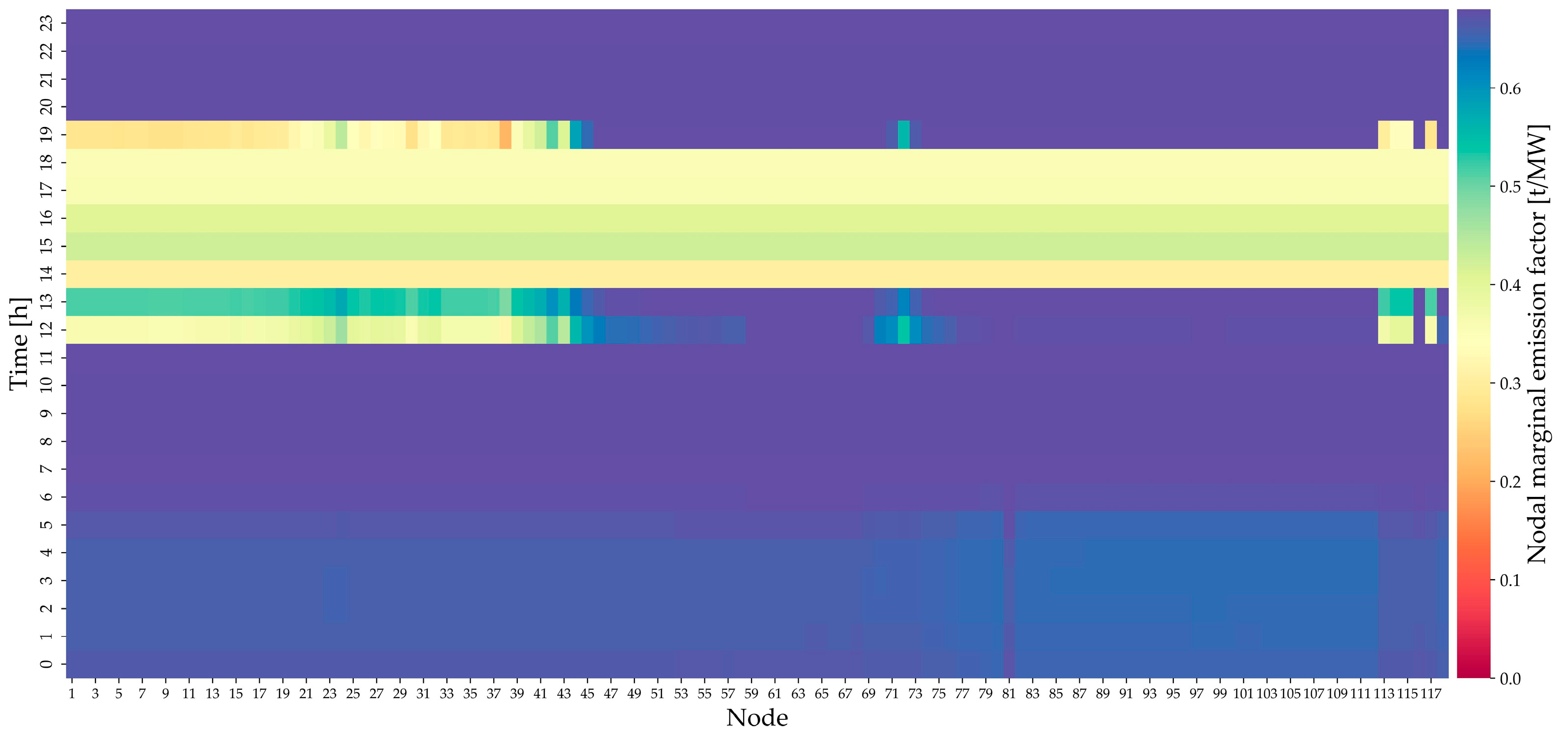
Figure 3 shows the NMEF results throughout the 24 h of 6 July using a heatmap. The horizontal axis represents nodal numbers 1–118. The vertical axis represents the time progression from 0 to 23 h. Different colors within the heatmap indicate the NMEFs at each node. As shown in the figure, during the high-load period from 12 to 19 o’clock, most nodes’ marginal carbon emissions remained within the stable range of 0.2–0.4 t/MW, indicating that increasing the load by 1 MW results in a relatively low NMEF. Continuing increasing demand at those nodes will not incur high emissions from 12 to 19 o’clock. However, some nodes (e.g., node 81) experienced a sharp increase in the NMEF to 0.6 t/MW and above throughout the early morning and evening. The reason for this scenario was network congestion; a high NMEF value indicates that a decrease in demand on those loads could reduce carbon emissions significantly.
According to Figure 3, four typical times are selected—early morning (05:00), afternoon (13:00), evening (19:00), and the absolute peak time of the day (16:00). The detailed NMEF results for those four typical times are shown in Figure 4.
In Figure 4, the blue bars represent NMEFs and the orange line indicates the ACE values. At 05:00 and 16:00, NMEFs of all nodes are lower than the system ACE and perform minimal differences. However, at 13:00 and 19:00, pronounced spatial heterogeneity emerges. Particularly for nodes 20 to 80, NMEFs are significantly different. For nodes 58 to 67, their NMEF exceeds the ACE. The carbon emission hot spots are identified on the power system topology. By viewing the detailed power flow results, we find that network congestion and the local generator status are the reasons for these spatial-induced NMEF differences.
Further, according to Figure 3, nodes 38, 65, and 81 present different NMEF profiles throughout 24 h. The detailed analysis for those five nodes is shown in Figure 5.
Figure 5 shows the NMEF values significantly change throughout 24 h for those three nodes. Before 11 o’clock, the profiles of the NMEF and ACE show a contrary tendency, i.e., when ACE is high, NMEF is low, and vice versa. During the afternoon period, the NMEF values for most nodes are significantly lower than the ACE values. This implies that those nodes could accept more demand without increasing the total carbon emissions significantly. These characteristics could be considered in power system unit-commitment for efficiently controlling overall carbon emissions. Second, nodes 65 and 81 experience a sharp increase in NMEF at 19:00. This is caused by transmission congestion, where power plants with lower emission rates cannot respond to the load change on nodes 65 and 81.
3.3. Fitting Characteristic Equations Using the GNN Model
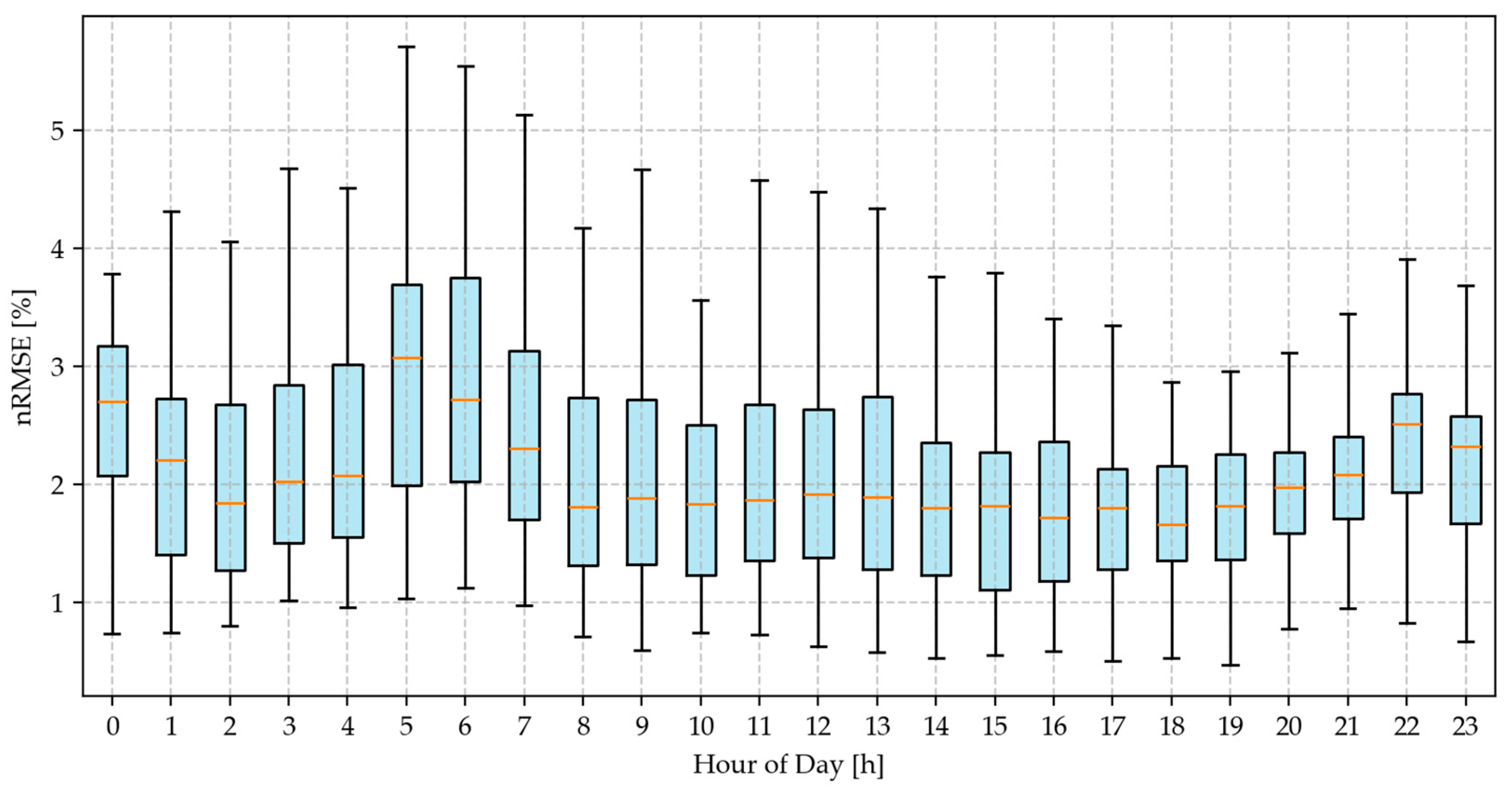
By mapping the load demand, voltage angle, generator output, node-level carbon emissions, renewable generation (wind and solar), generator type, system-level carbon indicators (total and average emissions), and total power generation to the NMEF via the GNN model, the characteristics of NMEF have been developed. To assess the temporal accuracy of the model, Figure 6 presents the hourly distribution of the nRMSE across all nodes in the system.

Figure 6.
Hourly nRMSE distribution across days.
Figure 6 is a boxplot of hourly nRMSE values for NMEF estimation across all nodes. Each box represents the distribution of nRMSE values for a given hour of the day. It can be observed that the estimation error exhibits a noticeable diurnal pattern. The median nRMSE remains between 1.8% and 2.8% throughout the day, indicating generally high estimation accuracy. However, peak values are observed around 06:00 to 08:00, coinciding with the system’s load ramp-up period. Lower error levels in the evening hours suggest that the model performs more stably during steady-state operation.
Figure 7 complements the nRMSE results by illustrating the variation in the nMAE. A similar pattern emerges, with the lowest median nMAE being around 1.5% during midday and the highest values (~2.5–3%) occurring during the early morning and late evening.
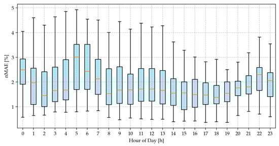
Figure 7.
Hourly nMAE distribution across days.
The reason for the high nRMSE and nMAE during the early morning hours is the sharp increase in total system demand due to residential and commercial activity. More notably, this period is also characterized by a significant injection of renewable energy, particularly solar and wind sources, coming online around sunrise. As a consequence, the dispatchable thermal generation—especially fast-ramping gas and coal-based cycling units—undergoes substantial modulation to balance the system. Such conditions lead to frequent and rapid dispatch changes in marginal generators, nonlinear emission responses due to generator fuel consumption curves, startup effects, and temporal asynchrony between renewable spikes and load increases. These dynamics collectively induce high volatility in the NMEF, which poses challenges for data-driven models trained on smooth historical patterns.
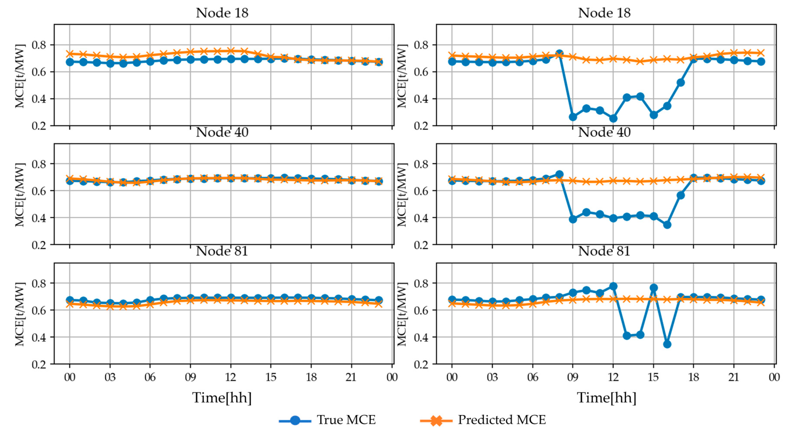
A node-level analysis further confirms this observation. Figure 8 presents the estimated versus actual NMEF at three representative nodes (node 18, node 40, and node 81) over two consecutive days: 6 July (left column) and 7 July (right column). The estimations are generated using the proposed GNN model.
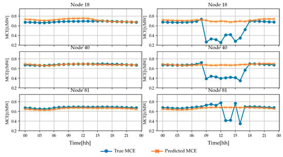
Figure 8.
NMEF estimation on 6 July and 7 July.
A clear contrast emerges between the two days. On 6 July, the model demonstrates high accuracy across all three nodes, with the estimated NMEF values closely tracking the true NMEF values throughout the 24 h. This indicates that under relatively stable system conditions, the model generalizes well across both spatial and temporal dimensions. For 7 July, however, a noticeable degradation in estimation accuracy is observed—particularly between 06:00 and 09:00, and again from around 13:00 to 16:00. This discrepancy is most pronounced at node 18 and node 40, where the estimated NMEF significantly underestimates the true values, even dropping below 0.3 t/MW, while the actual emissions remain around 0.7–0.75 t/MW.
To evaluate the generalizability of the proposed model across different geographical and topological regions of the power system, we have conducted a comparative analysis on five typical nodes—nodes 18, 38, 65, 81, and 112. These nodes were selected to capture diversity in load characteristics, generation mix, and line capacity.
Table 3 summarizes the estimation performance of four models: Long Short-Term Memory (LSTM), AutoRegressive Integrated Moving Average (ARIMA), Least Absolute Shrinkage and Selection Operator (LASSO), and the proposed GNN, evaluated using the nRMSE and nMAE. Across all five nodes, we observe that the GNN model consistently outperforms traditional time-series (ARIMA), statistical regression (LASSO), and even deep sequence models (LSTM).
Table 3.
Comparison of GNN and baseline models.
In addition to its superior estimation accuracy across representative nodes, the GNN model exhibits a key structural advantage over traditional and sequence-based models: it enables the simultaneous, parallel estimation of the NMEF for all nodes in the network. The GNN model leverages the global topological structure encoded in the graph representation of the power grid. This architectural design not only improves computational efficiency but also enhances coherence in emission estimation across interconnected nodes.
3.4. Discussion
Having the nodal marginal emission factor (NMEF) could support network operators understands the dynamic share of demand-induced emission responsibility among different nodes in power systems, therefore designing short-term scheduling strategies to enhance power-to-emission efficiency. For example, for nodes with a great NMFE at a given time, incentivizing demand to reduce demand on this node could reduce the NMFE and further reduce the average emission factor. On the contrary, for nodes with a low NMEF at a given time, if properly increasing demand on such nodes would not exponential increase the NMEF, incentivizing demand to increase demand could also reduce the overall emission factor for power systems, thus enhancing the power-emission efficiency.
In the long term, understanding the NMEF, such as in Figure 6 and Figure 7, could support network operators in setting targeted renewable and storage system planning. Low-NMEF targeted planning could reduce the NMEF by the inherent operational ability of distribution systems, therefore reducing the low-carbon operational pressure from transmission systems. Particularly when the objectives of reducing emission and reducing operational costs come into conflict, such as in Figure 5, during the 14:00–18:00 time period, the NMEF values for most nodes are significantly lower than the ACE values. This is caused by the starting up of low-emission but costly gas turbines to match the increasing demand. If effective and sustainable de-loading strategies, such as demand-side response and storage systems, are planned within those connected distribution networks, the demand for transmission networks will be reduced, thus reducing the reliance on gas turbines throughout the peak period. A win–win solution of low carbon and low cost scenario is reached.
4. Conclusions
This paper provides a carbon emission quantification framework centered on the NMEF, which breaks through the limitations of traditional ACE methods in terms of insufficient resolution and LCA macro-statistics, and significantly optimizes the CEF calculation process. The model characterizes carbon emission flows from the generator side to the demand side, clearly presenting the conversion method and allocation mechanism of the NMEF. Using the IEEE 118-node test system as an example, case studies have validated the accuracy and effectiveness of the model; deeply analyzed the fine-grained impacts of transmission congestion, power generation combinations, and load fluctuations on carbon emissions at each node; and revealed the hidden marginal extremum issues and their causes of deviation under the ACE method. Furthermore, compared to other models, the GCN can estimate the NMEF for all nodes at once and can achieve a 5.75% nRMSE and 2.52% nMAE. Last but not least, this paper brings a new finding. Under extreme cases, such as throughout the period of the yearly maximum demand, the marginal emission rates significantly drop for the majority of nodes. This is caused by the operation of flexible and low-emission but costly power generation units in the system. This finding raises a new argument: a strong inclination to reduce marginal emission rates might not be economically feasible in power system operation and planning. This argument suggests that to ensure low emissions and fuel cost emission, cost and emission efficient technologies should be considered, such as in demand-side response, distributed energy resources, and so forth.
Author Contributions
Conceptualization, B.F. and S.C.; methodology, B.F., J.Z. and S.C.; software, B.F., S.W. and L.L.; validation, B.F. and S.C.; formal analysis, J.Z. and L.L.; investigation, S.C.; resources, B.F. and S.C.; data curation, J.Z. and S.W.; writing—original draft preparation, B.F., J.Z. and S.C.; writing—review and editing, B.F. and L.L.; visualization, M.W. and L.L.; supervision, B.F. and S.C.; project administration, S.C. All authors have read and agreed to the published version of the manuscript.
Funding
This paper was funded by the Science and Technology Project of China Southern Power Grid Company Limited, grant number: 070000KC23110018.
Data Availability Statement
Publicly available datasets were analyzed in this study.
Conflicts of Interest
The authors Bing Fang, Jiayi Zhang, Shanli Wang, and Mingzhe Wen were employed by the company Hainan Power Grid Co., Ltd. The remaining authors declare that the research was conducted in the absence of any commercial or financial relationships that could be construed as potential conflicts of interest.
Nomenclature
| Time | |
| Node | |
| Node in the system | |
| Node for demand | |
| Node for renewable energy generator | |
| Node for solar power station | |
| Node for wind farm | |
| Node for gas generator | |
| Node for coal generator | |
| The output power for the solar power station at time | |
| The output power for the wind farm at time | |
| The output power for the gas generatorat time | |
| The output power for the coal generator at time | |
| Fuel price weight aligned to carbon emissions from coal generators | |
| Fuel price weight aligned to carbon emissions from gas generators | |
| Carbon emission from the coal generator at time | |
| Weight for the carbon emission function for the coal generator | |
| Weight for the carbon emission function for the coal generator | |
| Weight for the carbon emission function for the coal generator | |
| Carbon emission from the gas generator at time t | |
| Weight for the carbon emission function for the gas generator | |
| Weight for the carbon emission function for the gas generator | |
| Weight for the carbon emission function for the gas generator | |
| Demand connected to the node at time | |
| Power flows from node to its connected node at time | |
| Phase angle of node at time | |
| Phase angle of node at time | |
| Reactance of the transmission line between node and | |
| Maximum capacity of the transmission line between node and | |
| Minimum output power of the solar power station at time | |
| Maximum output power of the solar power station at time | |
| Minimum output power of the wind farm at time | |
| Maximum output power of the wind farm at time | |
| Minimum output power of the gas generator at time | |
| Maximum output power of the gas generator at time | |
| Minimum output power of the coal generator at time | |
| Maximum output power of the coal generator at time | |
| Demand of at time under base system | |
| System carbon emission under base system | |
| Marginal demand for at time | |
| System carbon emissions under marginal demand status | |
| The nodal marginal emission factors for the | |
| The adjacency matrix with added self-connections | |
| The diagonal degree matrix of | |
| The input feature matrix at layer | |
| The learnable weight matrix of layer | |
| Nonlinear activation function | |
| The parameter matrices and bias vectors of update gate | |
| The parameter matrices and bias vectors of update gate | |
| The previous time step’s hidden state of update gate | |
| The input of update gate | |
| The parameter matrices and bias vectors of reset gate. | |
| The parameter matrices and bias vectors of reset gate. | |
| The batch size of the training model. |
References
- Holland, S.P.; Kotchen, M.J.; Mansur, E.T.; Yates, A.J. Why marginal CO2 emissions are not decreasing for US electricity: Estimates and implications for climate policy. Proc. Natl. Acad. Sci. USA 2022, 119, e2116632119. [Google Scholar] [CrossRef] [PubMed]
- Hawkes, A. Long-run marginal CO2 emissions factors in national electricity systems. Appl. Energy 2014, 125, 197–205. [Google Scholar] [CrossRef]
- Zhang, Y.; Yang, X.; Fang, L.; Lyu, Y.; Xiong, X.; Zhang, Y. Data-Driven Day-Ahead Dispatch Method for Grid-Tied Distributed Batteries Considering Conflict Between Service Interests. Electronics 2024, 13, 4357. [Google Scholar] [CrossRef]
- Gil, H.A.; Joos, G. Generalized Estimation of Average Displaced Emissions by Wind Generation. IEEE Trans. Power Syst. 2007, 22, 1035–1043. [Google Scholar] [CrossRef]
- Zhang, X.; Zhu, H.; Cheng, Z.; Shao, J.; Yu, X.; Jiang, J. A review of carbon emissions accounting and prediction on the power grid. Electr. Eng. 2025. [Google Scholar] [CrossRef]
- Marrasso, E.; Roselli, C.; Sasso, M. Electric efficiency indicators and carbon dioxide emission factors for power generation by fossil and renewable energy sources on hourly basis. Energy Convers. Manag. 2019, 196, 1369–1384. [Google Scholar] [CrossRef]
- Liu, J.; Zhao, H.; Wang, S.; Liu, G.; Zhao, J.; Dong, Z.Y. Real-time emission and cost estimation based on unit-level dynamic carbon emission factor. Energy Convers. Econ. 2023, 4, 47–60. [Google Scholar] [CrossRef]
- Harrison, G.P.; Maclean, E.J.; Karamanlis, S.; Ochoa, L.F. Life cycle assessment of the transmission network in Great Britain. Energy Policy 2010, 38, 3622–3631. [Google Scholar] [CrossRef]
- Arvesen, A.; Hauan, I.B.; Bolsøy, B.M.; Hertwich, E.G. Life cycle assessment of transport of electricity via different voltage levels: A case study for Nord-Trøndelag county in Norway. Appl. Energy 2015, 157, 144–151. [Google Scholar] [CrossRef]
- Zhang, Y.; Liu, T.; Yao, L.; Song, Q.; Gao, C. Negligible carbon costs of UHVDC infrastructure delivering renewable electricity. Resour. Conserv. Recycl. 2023, 192, 106940. [Google Scholar] [CrossRef]
- Bai, M.; Li, C. Research on the allocation scheme of carbon emission allowances for China’s provincial power grids. Energy 2024, 299, 131551. [Google Scholar] [CrossRef]
- Wu, X.; Yang, W.; Zhang, N.; Zhou, C.; Song, J.; Kang, C. A Distributed computing algorithm for electricity carbon emission flow and carbon emission intensity. Prot. Control. Mod. Power Syst. 2024, 9, 138–146. [Google Scholar] [CrossRef]
- Kang, C.; Zhou, T.; Chen, Q.; Wang, J.; Sun, Y.; Xia, Q.; Yan, H. Carbon Emission Flow from Generation to Demand: A Network-Based Model. IEEE Trans. Smart Grid 2015, 6, 2386–2394. [Google Scholar] [CrossRef]
- Cheng, Y.; Zhang, N.; Wang, Y.; Yang, J.; Kang, C.; Xia, Q. Modeling Carbon Emission Flow in Multiple Energy Systems. IEEE Trans. Smart Grid 2018, 10, 3562–3574. [Google Scholar] [CrossRef]
- Yang, C.; Liu, J.; Liao, H.; Liang, G.; Zhao, J. An improved carbon emission flow method for the power grid with prosumers. Energy Rep. 2022, 9, 114–121. [Google Scholar] [CrossRef]
- Wang, Y.; Qiu, J.; Tao, Y.; Zhao, J. Carbon-Oriented Operational Planning in Coupled Electricity and Emission Trading Markets. IEEE Trans. Power Syst. 2020, 35, 3145–3157. [Google Scholar] [CrossRef]
- Bergh, K.V.D.; Delarue, E.; D’Haeseleer, W. Impact of renewables deployment on the CO2 price and the CO2 emissions in the European electricity sector. Energy Policy 2013, 63, 1021–1031. [Google Scholar] [CrossRef]
- Siler-Evans, K.; Azevedo, I.L.; Morgan, M.G. Marginal Emissions Factors for the U.S. Electricity System. Environ. Sci. Technol. 2012, 46, 4742–4748. [Google Scholar] [CrossRef]
- Koebrich, S.; Cofield, J.; McCormick, G.; Saraswat, I.; Steinsultz, N.; Christian, P. Towards objective evaluation of the accuracy of marginal emissions factors. Renew. Sustain. Energy Rev. 2025, 215, 115508. [Google Scholar] [CrossRef]
- Deetjen, T.A.; Azevedo, I.L. Reduced-Order Dispatch Model for Simulating Marginal Emissions Factors for the United States Power Sector. Environ. Sci. Technol. 2019, 53, 10506–10513. [Google Scholar] [CrossRef]
- Zhang, Y.; Zhu, X.; Liu, D.; Shan, Y.; Wu, Y. Marginal abatement cost of urban emissions under climate policy: Assessment and projection for China’s 2030 climate target. Sustain. Cities Soc. 2025, 124, 106319. [Google Scholar] [CrossRef]
- Wang, Y.; Qiu, J.; Tao, Y. Optimal Power Scheduling Using Data-Driven Carbon Emission Flow Modelling for Carbon Intensity Control. IEEE Trans. Power Syst. 2021, 37, 2894–2905. [Google Scholar] [CrossRef]
- Shi, H.; Fang, L.; Chen, X.; Gu, C.; Ma, K.; Zhang, X.; Zhang, Z.; Gu, J.; Lim, E.G. Review of the opportunities and challenges to accelerate mass-scale application of smart grids with large-language models. IET Smart Grid 2024, 7, 737–759. [Google Scholar] [CrossRef]
- Pena, I.; Martinez-Anido, C.B.; Hodge, B.-M. An Extended IEEE 118-Bus Test System with High Renewable Penetration. IEEE Trans. Power Syst. 2017, 33, 281–289. [Google Scholar] [CrossRef]
- Nguyen, N.A.; Vo, D.N.; Nguyen, T.T.; Duong, T.L.; Hong, T. An Improved Equilibrium Optimizer Algorithm for Solving Optimal Power Flow Problem with Penetration of Wind and Solar Energy. Int. Trans. Electr. Energy Syst. 2022, 2022, 7827164. [Google Scholar] [CrossRef]
- Liu, F.; Zhan, L.; Liu, Y. Determination of Load Characteristic of Standard Coal Consumption Rate in Coal-fired Generator Unit by One-point, Two-point and Multi-point Methods. J. Eng. Therm. Energy Power/Reneng Dongli Gongcheng 2021, 36, 73–80. [Google Scholar] [CrossRef]
- Cui, L.-L.; Li, Y.-F.; Long, P. Study on Coal Consumption Curve Fitting of the Thermal Power Based on Genetic Algorithm. J. Power Energy Eng. 2015, 3, 431–437. [Google Scholar] [CrossRef]
- Zakrzewski, T.; Stephens, B. Updated generalized natural gas reciprocating engine part-load performance curves for cogeneration applications. Sci. Technol. Built Environ. 2017, 23, 1151–1158. [Google Scholar] [CrossRef]
- Ausgrid Ltd. Distribution Zone Substation Data. Available online: https://www.ausgrid.com.au/Industry/Our-Research/Data-to-share/Distribution-zone-substation-data (accessed on 1 March 2025).


Disclaimer/Publisher’s Note: The statements, opinions and data contained in all publications are solely those of the individual author(s) and contributor(s) and not of MDPI and/or the editor(s). MDPI and/or the editor(s) disclaim responsibility for any injury to people or property resulting from any ideas, methods, instructions or products referred to in the content. |
© 2025 by the authors. Licensee MDPI, Basel, Switzerland. This article is an open access article distributed under the terms and conditions of the Creative Commons Attribution (CC BY) license (https://creativecommons.org/licenses/by/4.0/).