Predictive Maintenance of Proton-Exchange-Membrane Fuel Cells for Transportation Applications

Abstract

Proton-Exchange-Membrane Fuel Cell (PEMFC) systems are proving to be a promising solution for decarbonizing various means of transport, especially heavy ones. However, their reliability, availability, performance, durability, safety and operating costs are not yet fully competitive with industrial and commercial systems (actual systems). Predictive maintenance (PrM) is proving to be one of the most promising solutions for improving these critical points. In this paper, several PrM approaches will be developed considering the constraints of actual systems. The first approach involves estimating the overall State of Health (SOH) of a PEMFC operating under a dynamic load according to an FC-DLC (Fuel Cell Dynamic Load Cycle) profile, using a Health Indicator (HI). This section will also discuss the relevance of current End-of-Life (EoL) indicators by putting the performance, safety and economic profitability of PEMFC systems into perspective. The second approach involves predicting the voltage of the PEMFC while operating under this same profile in order to estimate its overall Remaining Useful Life (RUL). Finally, the last approach proposed will make it possible to estimate the time when it will be worthwhile, or even economically necessary, to replace a degraded PEMFC with a new one.

1. Introduction

In the coming years, access to the State of Health (SOH) will become essential to facilitate the purchase or resale of battery-powered electric vehicles. In light of this challenge, the European Union is planning to amend its legislation to simplify access to this crucial parameter. Similarly, precise access to the SOH for PEMFC-equipped vehicles will become a major challenge. However, the direct transcription of the SOH designation used on batteries to PEMFCs seems tricky. For batteries, the SOH can be estimated as the residual capacity of the battery. So, using a percentage description is understandable. For PEMFCs, however, it does not seem possible to do the same thing as for batteries, as the residual operating capacity comes from various criteria, such as electrochemical surface area, membrane thickness and corrosion of the catalytic support. Consequently, in this paper, the metric used to determine the SOH of PEMFCs will be the Health Indicator (HI). In the literature, determining the HI for PEMFCs under a constant load profile is not a problem [1]. However, determining it accurately with highly dynamic load profiles, intrinsic to transportation usages, is not an easy task. Similarly, when it comes to estimating the Remaining Useful Life (RUL) of a PEMFC operating under a dynamic load, there are difficulties in determining the overall RUL. Estimating the SOH and predicting the RUL of a PEMFC are key tools for guaranteeing the reliability and availability and reducing the operating costs of hydrogen systems [2]. This enables us to anticipate maintenance operations and intervene only when strictly necessary, avoid costly breakdowns, adapt operating conditions to improve durability, and better manage replacements. Industrial and commercial PEMFC systems (actual systems) generally operate under dynamic currents, so it is necessary to be able to estimate the overall SOH and predict the overall RUL. In the literature, numerous papers have focused on predicting the Remaining Useful Life (RUL) of PEMFCs under constant load using data-driven methods. Gibey et al. [2] and Chanal et al. [3] applied data-driven approaches for PEMFC RUL prediction, including a Multi-Reservoir Bidirectional Echo State Network (MR-BiESN), BiESN, and Bidirectional Long Short-Term Memory (BiLSTM), to predict RUL under constant load conditions. MR-BiESN outperformed BiLSTM, requiring 1200 times fewer parameters to optimize. K. Chen et al. [4] proposed a PEMFC RUL prediction method using Principal Component Analysis (PCA) and Gaussian Process Regression (GPR). RUL prediction using GPR showed that the PCA-GPR Rational Quadratic Kernel and PCA-GPR Exponential Kernel achieved the best accuracy. Zhang et al. [5] developed a Self-Adaptive Digital Twin (SADT) for PEMFC RUL prediction, using a deep CNN to generate stable Health Indicators across varying conditions. They introduced a Quantile Huber loss function (QH-loss) and applied transfer learning to improve accuracy and adaptability. L. Chen et al. [6] proposed a hybrid PEMFC RUL prediction approach combining mode decomposition and a two-phase deep learning model for RUL prediction. Their method, which processes low- and high-frequency components with BiLSTM and CNN, respectively, showed improved accuracy. However, all of these methods [2,3,4,5,6] have only been validated for a constant load. In the literature, only a few papers have developed approaches that are more-or-less satisfactory to estimate the overall HI and overall RUL of a PEMFC that has operated under a dynamic load. Zuo et al. [7] developed a method using a Fuel Cell Dynamic Load Cycle (FC-DLC) profile, testing models like LSTM, GRU, and their attention-enhanced versions. These models showed promising results for dynamic load but did not combine RULs at each point to trace the overall RUL. Morizet et al. [8] proposed a method for predicting the RUL of a PEMFC under a dynamic load by re-indexing physical time based on the accumulated load current. Predictions were made for different current ranges and combined to estimate the overall RUL. ESN with linear regression provided the best prediction performance. Tamilarasan et al. [9] compared degradation and RUL prediction methods for PEMFCs using data from the IEEE PHM 2014 Data Challenge, with one PEMFC under constant current and the other with current ripples. They tested various algorithms, of which the Self-Attention Temporal Dual Discriminator Generative Adversarial Network (SAT-DD-GAN) outperformed the others in terms of reliability and predictive performance, mainly due to its use of dual discriminators and self-attention mechanisms. Zhu et al. [10] developed a method to quantify uncertainty in predicting PEMFC degradation under dynamic load, based on varying lengths of training data. They transformed time-domain voltage signals into frequency factors and used TimesNet to predict sequences in both domains. The TimesNet-GPR method outperformed others, including LSTM and GRU. The authors suggest combining this approach with an RUL prediction algorithm.

Table 1. Prediction approaches list.

Reference	Approach Type	Approach Purpose	Dynamic Load Profile?
Gibey et al. [2]	Data-driven	RUL prediction	No
Chanal et al. [3]	Data-driven	RUL prediction	No
K. Chen et al. [4]	Data-driven	RUL prediction	No
Zhang et al. [5]	Data-driven	RUL prediction	No
L. Chen et al. [6]	Hybrid	RUL prediction	No
Zuo et al. [7]	Data-driven	RUL prediction	Yes
Morizet et al. [8]	Data-driven	RUL prediction	Yes
Tamilarasan et al. [9]	Data-driven	RUL prediction	Yes
Zhu et al. [10]	Data-driven	Degradation prediction	Yes

shows the types of approaches and load profiles for each reference cited in this section.

In this article, data-driven methods are proposed. These approaches use measurements that are always available in actual systems, in this case, voltage and current density, to suit everyone. The idea is to develop a PrM tool that can be used on all actual hydrogen-energy systems. In the first part of the paper, the calculation of the overall SOH of a PEMFC, operating under dynamic currents (FC-DLC profile) for 1008 h, is proposed through an HI. It is shown that the highest current density induces the lowest SOH, so it is necessary to use the latter for global SOH calculation. This novelty redefines the SOH calculation of PEMFCs operating under dynamic currents, which no previous papers have managed to achieve effectively. In the second part of the article, RUL prediction is carried out using the previously defined hypothesis, i.e., using the highest current density, to predict the RUL. Filtering methods are employed to eliminate outliers, reduce the number of data to improve computation time, and smooth the data to recover the global trend rather than local disturbances (performance recovery phenomena and measurement noise). The idea is to recover only the global trend and not local disturbances, which are of no interest for RUL prediction. Next, an ARIMA model is applied to predict the voltage for the highest current density in order to predict the overall RUL of the PEMFC. This model performs well in predicting linear time series, although it is necessary to carry out the various filtering steps mentioned above in order to eliminate non-linear behavior while preserving the data structure. More importantly, the ARIMA model allows for automated parameter setting, making it particularly interesting as a predictive maintenance (PrM) tool intended for commercial use by manufacturers. In contrast, current approaches typically rely on neural networks, whose parameters cannot be directly tuned within the system. These algorithms require manual tuning in advance, and their parameters must be adjusted over time to account for aging, which significantly increases the overall costs. The novelty of this approach is in the use of the overall SOH, the filtering steps prior to RUL prediction and the application of the ARIMA model with an automated parameter setting. In the third and final part of the paper, a maintenance scheduling optimization method for a PEMFC is proposed to precisely determine the replacement date of a degraded PEMFC, taking economic considerations into account. No articles in the literature have proposed such an innovative approach. Finally, the conclusions and perspectives for future work are presented.

2. PEMFC HI Estimation for Transportation Applications

Access to the HI for PEMFCs is an essential step in ensuring that the system can continue its mission under normal performance, reliability and safety conditions. Access to the SOH enables problems to be anticipated before they lead to a critical breakdown, or even a safety incident. In addition, it enables us to move from preventive maintenance (intervention according to a precise schedule) to PrM, which has several advantages, such as reducing maintenance costs by intervening only when strictly necessary, increasing system availability (less downtime) or extending the RUL by adapting control strategies to maximize the SOH. A PEMFC in poor condition no longer delivers the expected performance (current, power, efficiency). Monitoring the SOH makes it possible to adjust operating conditions in real time [11,12], as is carried out with batteries, to extend durability and maximize efficiency [13]. Electricity industry players already offer this type of functionality for batteries, but at present, none do so for hydrogen systems. Access to the HI for a PEMFCs operating under a variable current density, as is the case for heavy or light vehicles, has received very little attention in the literature. In this section, a data-driven method for diagnosing the HI of a PEMFC for transportation applications is proposed.

2.1. Data Processing

In order to diagnose the HI of a PEMFC, a dataset is required. The dataset used in this paper came from Zuo et al. [14]. The study analyzes the durability and long-term dynamic performance of a Proton-Exchange-Membrane fuel cell (PEMFC), with an active surface area of 25 cm², subjected to dynamic load profiles, according to an FC-DLC cycle. The tests, carried out at the Greenlight G20 test station, involved 3076 cycles over approximately 1008 h. The operating conditions included a cell temperature of 70 °C, with the hydrogen dew point set at 55 °C and the air dew point at 65 °C. The hydrogen and air inlet pressure was maintained at 110 kPa, while the cell operating humidity was controlled by humidifiers. Data acquisition was carried out at 1 Hz, recording parameters such as voltage, current, power, inlet and outlet pressures, gas flow rates and operating temperatures. This cycle is shown in Figure 1 and was repeated 3076 times. In addition, regular characterizations (polarization curves) were carried out every 100 h to provide information on PEMFC performance, aging and performance recovery phenomena. Given that actual PEMFC systems generally operate under dynamic currents, the choice was made to use this dataset for HI estimation and RUL prediction. The results obtained in this article provide a basis for validating the methodology, which will be validated on other datasets in future work.

Prior analysis of data (corresponding to data processing and filtering before data analysis) to determine the HI of a PEMFC under a dynamic load profile is essential to ensure reliable assessments of PEMFC health. Firstly, it is necessary to establish a baseline in order to determine the original HI of the PEMFC. Secondly, dynamic load profiles can generate noise in the data, due to the transient nature of current density variations. In particular, rapid transitions between different current density levels can affect the temperature and humidity distribution inside the PEMFC, thus altering the voltage measured for the same current density point. This noise may be due to sensor measurements, rapid load fluctuations, humidity variations or thermal effects. In addition to noise, it is necessary to consider performance recovery phenomena in order to assess the HI of the PEMFC as accurately as possible. It is then essential to filter the data while retaining relevant information on the state of the PEMFC so that the HI analysis is as reliable as possible. To achieve this, several methods can be considered, such as the averaging method, polynomial regression, a Savitzky–Golay filter [15] or an unscented Kalman filter [16]. Therefore, finding the overall HI of a PEMFC operating under a dynamic load requires prior data analysis. In the considered dataset, the voltages and operating times for each current density point were extracted. It should be pointed out that the extraction was carried out considering sensor errors and environmental noise, i.e., a hysteresis around the current density value was set up. In concrete terms, this hysteresis corresponds to a value of plus or minus 2.5% around the value of the current density, to ensure that it considers the above-mentioned disturbances. Moreover, under dynamic loading, this is taken into consideration, as when the current density value changes from, say, 0.828 A/cm² to 1.184 A/cm², the 2.5% hysteresis will be recalculated around the new current value. It should also be noted that this approach was successfully tested on the dataset used in this article. Next, the HI of the PEMFC per current density point was calculated by dividing the original voltage by the final voltage (for the same current density point, and expressed as a percentage). To take account of measurement errors and uncertainties, the original voltage was taken as the average of the first 1000 voltage measurements. Similarly, the final voltage was considered to be the average of the last 1000 voltage data points. The voltage drop percentage was calculated by subtracting the HI from the initial SOH of 100% (corresponding to the beginning of life). For each current density, the average voltage loss per cell per hour was calculated as the difference between the initial voltage and the final voltage, the result of which was divided by the operating time to obtain the voltage loss in V/cell/h. Finally, the final result was obtained by converting the voltage attenuation into µV (multiplying by ${10}^6$) to obtain the average voltage drop in µV/cell/h.

Table 2. Data analysis of a PEMFC operated under an FC-DLC profile to estimate the HI and average voltage loss for each current density.

Current [A]	Current Density [A/cm²]	Operating Time [h]	Initial Voltage [V]	Final Voltage [V]	HI [%]	Voltage Drop [%]	Average Voltage Loss [µV/cell/h]
0	0	29.9	0.943	0.919	97.45	2.55	802.68
1.78	0.0712	373.7	0.877	0.838	95.56	4.44	104.36
4.4	0.176	42.2	0.830	0.783	94.34	5.66	1113.74
9.5	0.38	111.8	0.783	0.721	92.08	7.92	554.56
10.4	0.416	81.2	0.780	0.718	92.05	7.95	763.55
14.8	0.592	129.5	0.746	0.672	90.08	9.92	571.43
20.7	0.828	115.5	0.706	0.623	88.24	11.76	718.61
29.6	1.184	40.3	0.640	0.554	86.56	13.44	2134
35.5	1.42	35.8	0.596	0.511	85.74	14.26	2374.3

shows the results obtained for each current density point. It should be pointed out that the End-of-Life (EoL) threshold for a PEMFC depends on the intended application, and is set at 10% HI loss for light vehicles and 20% HI loss for heavy vehicles, stationary applications and μ-CHP [17].

2.2. Diagnostic Results

The analysis of the voltage and operating time data for each current density point provides information on the variation in the HI of the PEMFC. Figure 2 shows the HI obtained after 1008 h of operation for each current density point. It can be seen that the higher the current density value, the lower the HI, irrespective of the operating time. The PEMFC ran for 35.8 h at 1.42 A/cm² and for 373.7 h at 0.0712 A/cm², with HI values of 85.74% and 95.56%, respectively. The hours of operation per current density do not change the fact that the highest current density induces the lowest HI. This phenomenon is logical, because whatever the current density value, it degrades the PEMFC. In fact, even though the PEMFC operated for less time at higher current densities than at lower current densities, irreversible degradation, which is more pronounced at higher current densities, resulted in a lower HI at higher current densities. There are several possible explanations for these findings:

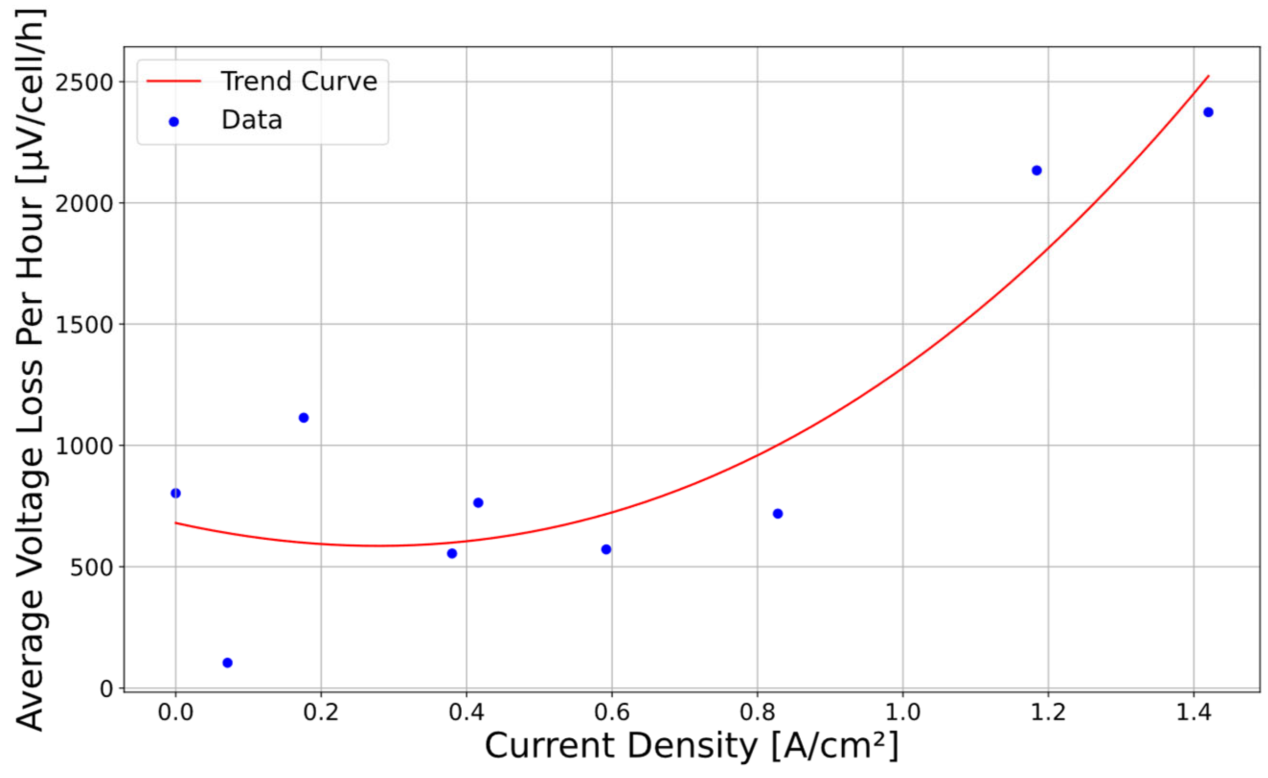
• Over time, the voltage decreases more rapidly at high current densities due to the accelerated degradation of PEMFC components such as the electrode, gas diffusion layer, bipolar plates and membrane.
• At a high current density, water production at the cathode is greater, resulting in poor water management and thus affecting the durability of the PEMFC.
• A high current density can cause mechanical stresses on the membrane as a result of the increased flow rate required to deliver the desired current density, thus accelerating PEMFC degradation.
• A high current density can accelerate corrosion of the carbon in the electrodes, thus speeding up degradation of the PEMFC.
• A high current density can promote the formation of free radicals, which attack the membrane, accelerating PEMFC degradation.

Figure 2. PEMFC HI for each current density point after 1008 h of operation.

Figure 2. PEMFC HI for each current density point after 1008 h of operation.

Figure 3 shows the average voltage loss per cell per operating hour per current density point. The average voltage loss for a current density of 0 A/cm² is 802.68 µV/cell/h, which is higher than for current densities of 0.0712 A/cm², 0.38 A/cm², 0.416 A/cm², 0.592 A/cm² and 0.828 A/cm², but not for a current density of 0.176 A/cm², for which the voltage loss value is 1113.74 µV/cell/h. This may be due to poor membrane hydration, for example. The average voltage loss then increases to 2134 µV/cell/h and 2374.3 µV/cell/h for 1.184 A/cm² and 1.42 A/cm², respectively. A PEMFC operating in an open circuit is subject to a set of electrochemical (high potentials), chemical (formation of reactive species) and mechanical (drying out or cracking) conditions that are extremely unfavorable and degrading. On the other hand, when a PEMFC works at high current densities (e.g., 1.42 A/cm²), the concentration and temperature gradients are high, humidification is difficult to control, the catalyst dissolves, ohmic losses increase, concentration losses can occur and mechanical stresses appear. As a result, degradation is quite significant at low current densities and intensifies sharply at high current densities. Finally, for 1.42 A/cm², which is the highest current density, the average voltage drop per hour is the greatest, indicating increased degradation of PEMFC performance during these phases. These results match those obtained for HI, which is lower for the highest current density of 1.42 A/cm². On the other hand, if, for example, in this cycle, 1.42 A/cm² was used twice as much, then an even lower HI would be found. These results are very interesting for estimating the overall HI of the PEMFC, which will then be that of the highest current density, for questions of performance, reliability and safety in particular. In concrete terms, if the overall HI is incorrectly estimated, i.e., by not using the highest current density, then this would lead to the upward overestimation of actual health status. In the case of a hydrogen bus, for example, the overestimation of health status would result in actual the performance being lower than expected. In fact, the bus’s PEMFC would be unreliable due to false information about errors when calculating HI. On the other hand, the bus might not be able to overtake correctly on the road, for example, creating safety problems for passengers and other motorists. It is then necessary to use the highest current density to calculate the HI, as this reflects the lowest HI. However, care must be taken with high current densities, which may no longer be accessible in the long term due to aging. In fact, the current density used to estimate the HI will be considered to be the maximum current density accessible and it will be used. Based on the various diagnostic results, a number of hypotheses can be put forward, which will be validated on other datasets in future work, in order to refute or confirm them.

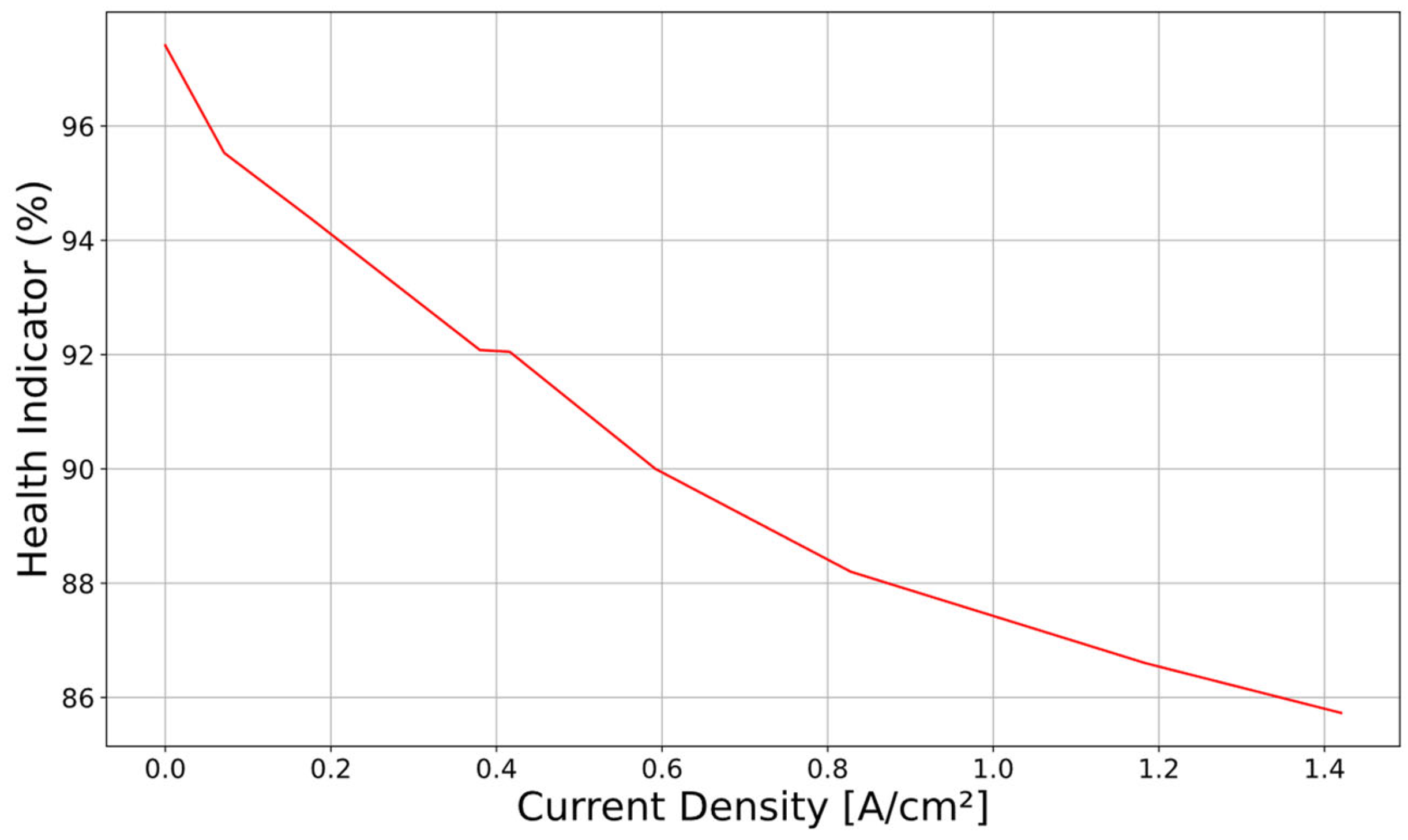
• Assumption 1: The highest current density will be used to calculate the system’s overall SOH, because we obtain the lowest SOH for this current point.
• Assumption 2: The operating time per current density point does not alter the fact that the highest current density point induces the lowest HI.

These assumptions do, however, suggest one possibility. Perhaps we are being too pessimistic by taking the highest current density, as this will impact the economic efficiency of the system. It would then be necessary to re-evaluate the standards used for EoL (10% or 20% relative power loss depending on the application) or to contact the manufacturers or users of PEMFC systems for transport to find out whether it is possible, for example, to tolerate a 75% HI for the highest current density in order to improve the economic efficiency of the system. Safety, reliability, performance and economic cost indicators certainly need to be refined.

Figure 3. PEMFC average voltage loss per hour for each current density point.

Figure 3. PEMFC average voltage loss per hour for each current density point.

3. PEMFC RUL Prediction for Transportation Applications

In the previous section, overall HI estimation of a PEMFC operating according to a dynamic profile was performed. In this section, the process of obtaining an overall RUL prognosis will be described, which made it possible to predict the RUL before the PEMFC was declared EoL. This step was necessary in order to anticipate maintenance interventions, in this case, PEMFC replacement, or modify control, leading to improved availability, durability, lifetime, reliability and safety in PEMFC systems. However, it should be pointed out that the RUL of PEMFCs is strongly influenced by the operating conditions. Liu et al. [18] explored various methods for limiting the deterioration of PEMFCs during start-up phases. It is reported that during a prolonged period of inactivity, the PEMFC anode becomes charged with air. When the PEMFC restarts, the introduction of hydrogen into the anode causes a hydrogen–air interface. On the other hand, after PEMFC shutdown, the anode fills up with oxygen due to the concentration gradient between the anode and cathode, and also due to the tightness of the system, maintaining a residual presence of hydrogen and creating a hydrogen–air interface once again. In operating situations involving stop–start cycles under dynamic conditions, a shift in and/or non-uniform distribution of reactants leads to local gas depletion. This phenomenon accentuates the concentration gradient, generating a hydrogen–air interface at the anode. Furthermore, high interfacial potential differences at the cathode promote oxygen precipitation and trigger carbon corrosion reactions. Ultimately, these shutdown-and-restart cycles contribute significantly to the degradation of PEMFCs. Pahon et al. [19] tested open-cathode PEMFCs stored at room temperature and below 0 °C. High-current tests showed reduced mass and charge transport efficiency due to ice formation, though the open-circuit voltage remained stable, indicating minimal membrane degradation. After two years, the performance dropped by 12% for room-temperature cells and 20% for sub-zero cells, highlighting the impact of cold storage on PEMFC durability. Alink et al. [20] studied PEMFCs after 120 freeze–thaw cycles in dry and 62 in wet conditions. Water phase transitions caused conductivity changes and membrane dehydration below 0 °C, reducing the active surface area and causing charge transfer losses. Electrode material detachment and damage to the gas diffusion layer were also observed. In this paper, it should be pointed out that these particular operating modes were not taken into consideration.

3.1. Data Processing and Algorithm Choice

In order to predict the overall RUL of a PEMFC, the highest current density, in this case, 1.42 A/cm², should be used, as it was shown in the previous section that this reflects the overall HI of the system. However, it should be pointed out that it is necessary to report the overall operating time of the system and not that reported for 1.42 A/cm² for RUL estimation. This is necessary because the system operates dynamically over several current density points. It is therefore necessary to report the overall operating time and not the operating time for this current density; otherwise, the results will be completely distorted (for example, an SOH of 85.74% after 35.8 h for 1.42 A/cm²). Nevertheless, the system has actually been operating for 1008 h. If we estimate the RUL without considering the overall operating time, we might think that there are around 14 h of operating time left (for an EoL declared at 80% of SOH), whereas in reality, there are around 400 h. In this section, the choice was made to use the AutoRegressive Integrated Moving Average (ARIMA) model [21]. This model is highly suitable for predicting time series with linear trends. For this reason, it is necessary to filter the data to avoid performance recovery and non-linear behavior, in order to obtain very good prediction accuracy. The various data processing steps performed before feeding the model are listed below:

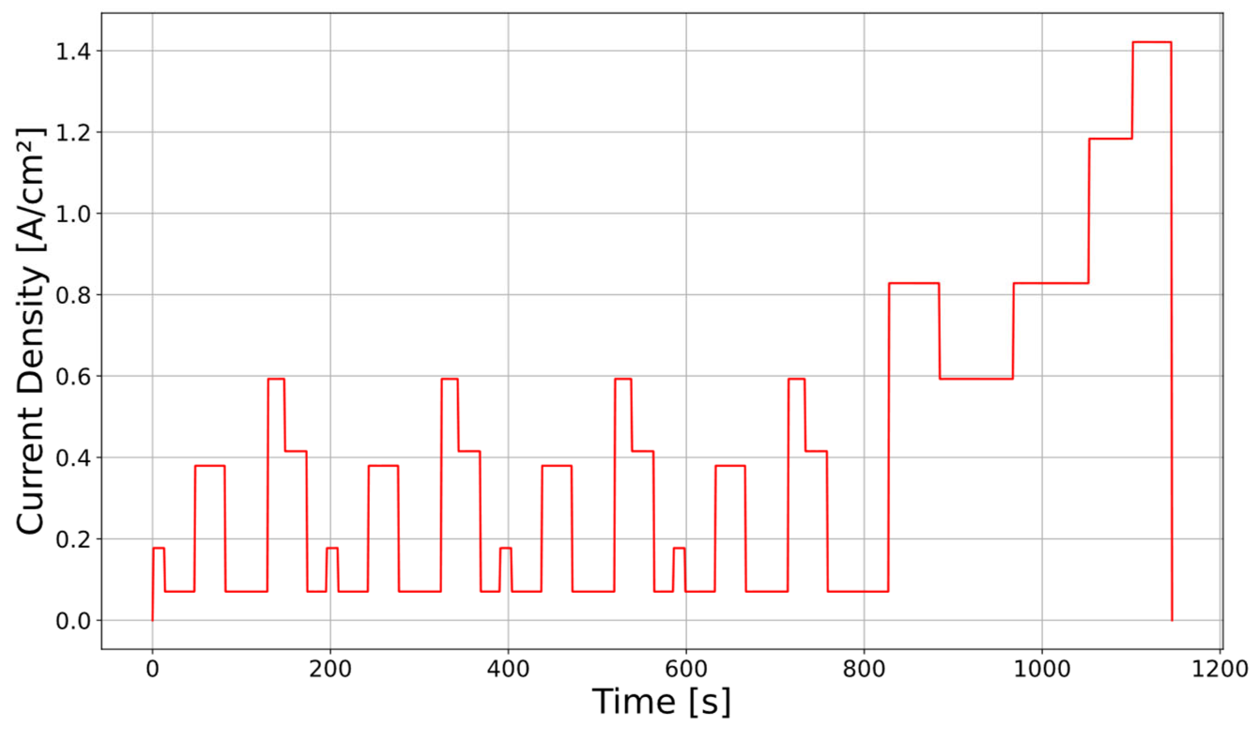
• We extracted the fuel cell voltage for the highest current density point, in this case, 1.42 A/cm² As demonstrated, it was necessary to recover only the voltage for the highest current density to obtain the overall SOH of the PEMFC. This voltage was used to predict the overall RUL.
• We extracted the overall fuel cell operating time. It was necessary to extract the overall operating time because the system operates dynamically over several current density points. If only the operating time for the maximum current density had been extracted, then it would have been impossible to find the system’s true RUL.
• We eliminated outliers using a logic filter. These outliers are generally due to measurement errors or system shutdown/breakdown, either because of a technical problem or to carry out characterization such as a polarization curve or an electrochemical impedance spectrum.
• We reduced the number of redundant data to significantly improve the computation time of the prediction algorithm. To achieve this, the raw voltage data were divided into n clusters. Then, for each cluster, the average was calculated. The n averages were then linked to create a new vector, which was considered the original data vector, named “Original Data” in Figure 4.
• We smoothed the data using the Savitzky–Golay filter to eliminate measurement noise and smooth the performance recovery phenomena. This filtering allowed us to recover the overall trend rather than local variations, which are of no interest when predicting the RUL.

It should be pointed out that data processing is a necessary step in obtaining good prediction performance and fast computing times compatible with real time.

3.2. Prognostic Results

After the data were processed, the ARIMA model was used to predict the PEMFC voltage in order to estimate its overall RUL. The data used for prediction were the same as in the previous section.

Table 3. Setting parameters and prognostic results.

	ARIMA (10%)	ARIMA (20%)
Setting parameters	Automatic optimization of polynomial orders Order found by automatic optimization: (0, 2, 3)	Automatic optimization of polynomial orders Order found by automatic optimization: (2, 2, 3)
Prediction horizon	372 h	223 h
Computation time	3.8 s	9.2 s
Estimated RUL	293 h	120 h
Real RUL	305 h	Unknown
Error between estimated and real RUL	12 h (0.98%)	Unknown

and Figure 4 show the tuning parameters and results obtained with this approach, respectively. In Figure 4, an increase in voltage is observed after 700 h. The loss in voltage is due to the degradation of the PEMFC; however, voltage recoveries can occur for a number of reasons, such as a performance recovery procedure, a characterization phase such as a polarization curve before cycling the system again, or improved membrane hydration. The authors of the dataset indicate that the characterization phases have contributed to deepening PEMFC performance recovery phenomena. However, this information alone does not really explain the voltage increase observed after 700 h. Other factors must have influenced this, such as better management of membrane hydration. It is for this reason in particular that the Savitzky–Golay filter was used, in order to recover the overall degradation trend, and not local performance recovery phenomena due to various factors. It should be pointed out that two predictions were made using the ARIMA model to suit all applications, the first to estimate the RUL when the PEMFC has lost 10% of its original power, the second for when it has lost 20%. The prediction starting point may slightly affect the prediction accuracy if the data are not well filtered beforehand. Nevertheless, in order to suit an industrial and commercial context, we chose to define the starting point arbitrarily between 200 h and 300 h before the EoL of 10% and 20%, respectively, with the aim being to validate the RUL estimate with a prediction horizon of at least 200 h, enabling maintenance interventions to be anticipated. On the other hand, it should be noted that the prediction starting point for unfiltered data would have a strong impact on the results of the ARIMA model, notably due to non-linear variations. As far as the learning window is concerned, all data preceding the prediction were used for model tuning.

It should be pointed out that the data did not reach a loss of 20% HI; nevertheless, a future prediction was made in order to estimate the operating time at which the system will have undergone a 20% HI loss. The prediction results were very good for the 10% HI loss, with an error of less than 1% for a prediction horizon of 372 h. In addition, the computation times for the predictions were 3.8 s and 9.2 s, respectively, enabling the predictions to be rerun to ensure their quality. Furthermore, this fast computation time makes it possible to carry out online retraining. This approach is an integral part of predictive maintenance (PrM) and is compatible with actual systems, as it has the following advantages:

• It uses always-available measurements (voltage, current and time).
• It has a fast computation time, so predictions can be rerun to ensure quality, and online re-training can also be carried out.
• It allows the automatic optimization of setting parameters.

The ARIMA is a linear model that has proven its effectiveness in predicting time series with linear trends [22]. However, for PEMFCs, non-linear behavior in the voltage data occurs, notably due to measurement noise and performance recovery phenomena. It is therefore necessary to perform filtering steps beforehand, for example, with the Savitzky–Golay filter, in order to smooth the data and recover only the overall trend. Figure 4 shows that this filtering step remains faithful to the data structure. In the case of highly non-linear data, data filtering may not be sufficient for the ARIMA model to perform well. In such a case, another model capable of handling this type of behavior could be used instead. However, the tuning parameters of this model need to be automated to match the objective of a PrM tool in actual systems. XGBoost regressor [23] seems to be a very good candidate for this purpose.

4. PEMFC Maintenance Scheduling Optimization

In the previous section, an RUL prognosis of a PEMFC operating according to a dynamic profile was obtained. In this section, an approach to optimizing the maintenance schedule in the context of PrM for PEMFC systems will be proposed. The idea is to define, as accurately as possible, the time from which it is most economically viable to replace a degraded PEMFC with a new one.

4.1. Methodology and Assumptions

To find the optimum date for replacing a PEMFC with a new one, we need to estimate the amount of hydrogen consumed by the PEMFC, taking aging into account. In other words, in order to ensure the same power output, the PEMFC will consume more hydrogen due to performance degradation. This extra consumption is then compared with hydrogen consumption without aging, i.e., for a new PEMFC. When the cumulated cost of excess hydrogen consumption exceeds the price of a new PEMFC, it makes economic sense to replace it. The various indicators used to find this date are as follows:

• PEMFC power [W].
• PEMFC HI [%].
• PEMFC operating time [h].
• Hydrogen consumed by the PEMFC [kg/h].
• PEMFC cost [EUR/kW].
• Hydrogen cost [EUR/kg].

The electrical power P in W represents the electrical energy produced by the PEMFC. In order to produce this power, a certain quantity of hydrogen is required. The efficiency η quantifies the losses incurred in converting chemical energy into electrical energy. The electrical power produced can be defined as follows:

$$\mathrm{P}=\eta \times Q_{m_{H2}}\times \mathsf{\Delta }\mathrm{H}.$$

(1)

where $Q_{m_{H2}}$ is the hydrogen mass flow rate in kg/s and $\mathsf{\Delta }$H is the hydrogen enthalpy of the reaction in J/kg. The energy contained in 1 kg of hydrogen Ψ is a constant equal to 33,000 Wh/kg [24]. So, the value of ΔH can be calculated as follows:

$$\mathsf{\Delta }\mathrm{H}=\Psi \times 3600=\mathrm{33,000}\times 3600=\mathrm{118,800,000}\mathrm{J}/\mathrm{kg}\approx 120\times {10}^6\mathrm{J}/\mathrm{kg}.$$

(2)

Next, $Q_{m_{H2}}$ must be isolated:

$$Q_{m_{H2}}={\displaystyle \frac{\mathrm{P}}{\mathsf{\eta }\times \mathsf{\Delta }\mathrm{H}}}.$$

(3)

To obtain the flow rate in kg/h, it is necessary to convert the initial mass flow rate into kg/s.

$$Q_{H2}=({\displaystyle \frac{\mathrm{P}}{\mathsf{\eta }\ast \mathsf{\Delta }\mathrm{H}}})\times 3600.$$

(4)

This equation can be formulated in another way, using the energy contained in 1 kg of hydrogen instead of the enthalpy of the reaction. This gives

$$Q_{H2}=({\displaystyle \frac{\mathrm{P}}{\mathsf{\eta }\ast \Psi }})\times 3600$$

(5)

To summarize, the hydrogen flow in kg/h can be calculated in two ways, using either Equation (6) or Equation (7).

$$Q_{H2}={\displaystyle \frac{P}{\eta \times \Psi }}$$

(6)

$$Q_{H2}=({\displaystyle \frac{P}{\eta \ast \mathsf{\Delta }H}})\times 3600$$

(7)

The electric efficiency depends on the PEMFC supplier and was set at 0.5 for the calculation (50%). The power depends on the PEMFC studied; in this case, a power of 1 kW was used. Certainly, these values could be modified according to the actual power and electrical efficiency values supplied.

It should be pointed out that with the data used previously for HI estimation and RUL prediction, no time can be found because the price of a PEMFC in EUR/kW is too high, its lifetime in hours too low and the price of hydrogen in EUR/kg too high. Nevertheless, these data give us information about the evolution of the HI for a current density point as a function of time. In Figure 5, the HI for the maximum current density of 1.42 A/cm² varies almost linearly with time. This assumption will be used for the following calculations.

Concerning hydrogen price, Eliseo Cursio [25] indicates that the current price of green hydrogen is between USD 3.5 and USD 6 per kg. However, this price range may increase due to several factors, such as the region of the world (due to the variable costs of renewable energy), the manufacturer, the scale of production (costs being higher on a small scale), hydrogen storage and transport (costs in addition to the selling price) and the technologies used. Furthermore, the author indicates that by 2030, prices should fall to between USD 2.5 and USD 3 per kg. Gül et Akyüz [26] indicate a price of between USD 1.98 and USD 3.82 per kg by 2050. Concerning PEMFC prices, Cigolotti et al. [27] analyzed the cost of PEMFCs in EUR/kW according to three power ranges (<5 kW, between 5 kW and 50 kW, and between 50 kW and 500 kW). For each power range, the price of a PEMFC was around 6 k EUR/kW, 2.5 k EUR/kW and 1.8 k EUR/kW, respectively, in 2020, around 4 k EUR/kW, 1.8 k/kW and 1.6 k EUR/kW, respectively, in 2024, and the prices will be around 3 k EUR/kW, 1.4 k EUR/kW and 0.6 k EUR/kW, respectively, in 2030. Whiston et al. [28] conducted a study to assess the cost of PEMFC operation for automotive applications. The experts estimated median costs of USD 75/kW, USD 62/kW and USD 46/kW for 2017, 2020 and 2035, respectively. However, for 2017, expert opinions diverged, with estimated price ranges between USD 40/kW and USD 500/kW. The actual prices of PEMFCs are therefore very complicated to estimate, as they depend on many factors, such as the scale of production, with costs being higher on a small scale, or the manufacturer.

The PEMFC maintenance scheduling optimization calculation was carried out considering several possible scenarios (current and future) for the price of hydrogen and PEMFCs, with variations of 2 EUR/kg, 4 EUR/kg, 6 EUR/kg, 8 EUR/kg, 10 EUR/kg and 12 EUR/kg and of 100 EUR/kW, 200 EUR/kW, 500 EUR/kW and 1000 EUR/kW, respectively. The assumptions for the calculations are as follows:

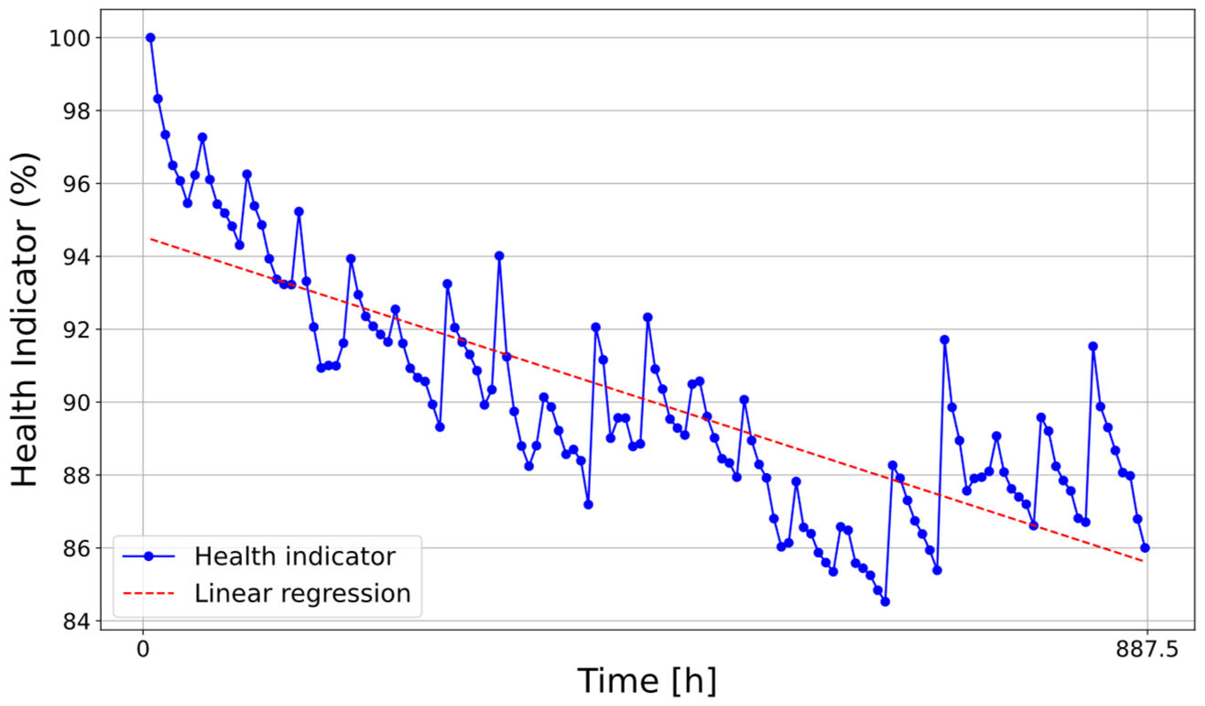
• HI is assumed to decrease linearly over time. This assumption is consistent with Figure 5.
• The EoL is declared when the PEMFC has lost 20% of its performance versus the beginning of life (heavy-duty vehicle application) after 10,000 h of operation.

The steps and equations used for the calculations in Figure 6 are as follows:

• Calculation of reference hydrogen flow (without aging) using Equation (6).
• Calculation of actual hydrogen flow rate as a function of SOH (with aging):

$$Q_i=Q_{H2}\times (1+{\displaystyle \frac{100-{SOH}_i}{100}})$$

(8)

• Calculation of additional hydrogen costs:

$${Additional\_costs}_i=(Q_i-Q_0)\times {Hydrogen}_{cost}$$

(9)

• Calculation of cumulative additional hydrogen costs:

$${Additional\_costs}_{cumulative}={\sum }_i{Additional\_costs}_i$$

(10)

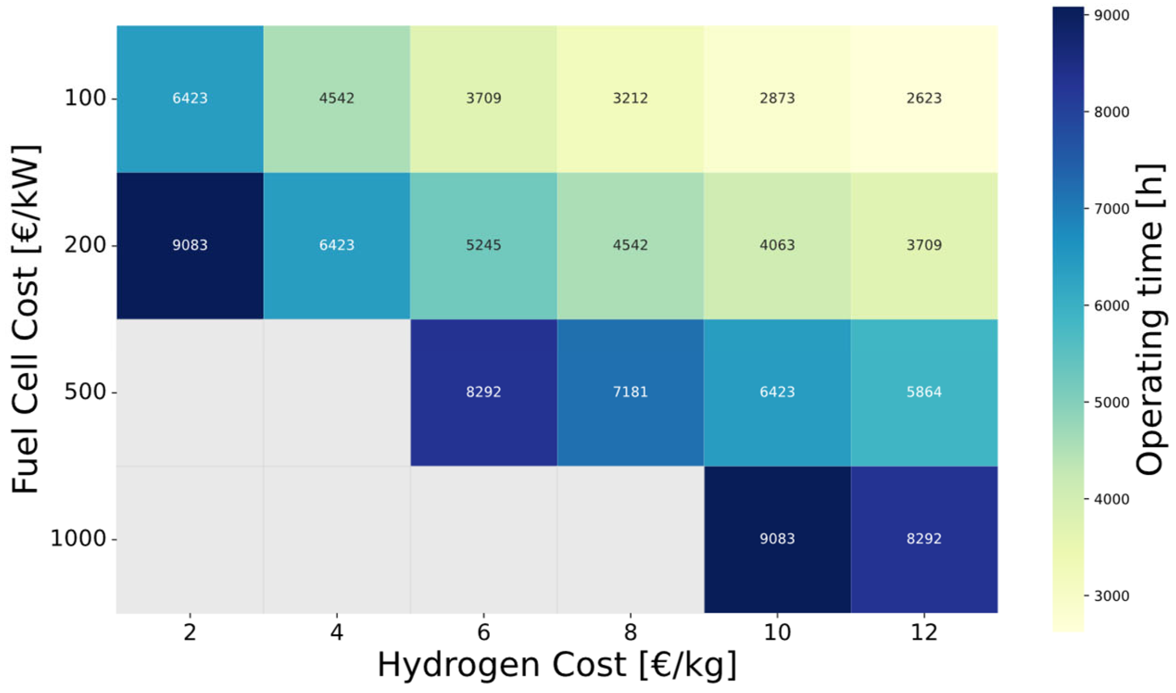
• If the cumulative extra cost exceeds the price of a new PEMFC, the time from which this occurred will be displayed in Figure 6. This date tells us that it is economically worthwhile, or even necessary, to replace the degraded PEMFC with a new one. On the other hand, if this has not occurred, no value will be displayed.

4.2. Results and Discussion

Figure 6 shows that of the 24 case studies proposed, only 6 do not require replacement of the PEMFC before its actual EoL, corresponding to an HI of 80%. Of these six cases, four are for a PEMFC costing 1000 EUR/kW with a hydrogen price ranging from 2 EUR/kg to 8 EUR/kg. These results are quite logical, given that the price of hydrogen is low and the price of the PEMFC is high, and the ratio between the additional cost of hydrogen consumed due to aging and the cost of hydrogen that would be consumed without aging never exceeds the price of the PEMFC. Similarly, the other two cases are for a PEMFC costing 500 EUR/kW at a hydrogen price of 2 EUR/kg and 4 EUR/kg. Conversely, the 18 other cases require the PEMFC to be changed before its actual EoL. The most convincing and obvious case is when the PEMFC is the cheapest and the hydrogen the most expensive, at 100 EUR/kW and 12 EUR/kg, respectively. In this case, it is advisable to change the PEMFC after only 2623 h of operation, i.e., slightly more than a quarter of the time (around 94.75% HI) of operation before its EoL. It should be pointed out that these results are a first attempt to implement the method, which will need to be coupled with HI estimation and RUL prediction in real time in order to be embedded in an actual system through the PrM tool. In the future, with research and industrialization, the price of hydrogen and the price of PEMFCs will fall sharply [25,26,27,28]. In such a scenario, PEMFCs are likely to be replaced before their actual EoL for economic reasons. We must also consider the ecological impact this could have, due to the waste of components that are still viable but too costly to conserve.

5. Conclusions

In this paper, several approaches integral to the PrM of PEMFCs were carried out. In the first part of the paper, the overall HI of a PEMFC operating under a dynamic load according to an FC-DLC profile was estimated. The lowest HI was found for the highest current density, irrespective of the operating time per current density point. It was therefore concluded that the highest current density should be used to estimate the overall HI of a PEMFC operating under a dynamic load, not least for performance, reliability and safety reasons. In the second part of this paper, PEMFC voltage prediction was carried out in order to estimate its overall RUL. Two predictions were carried out to suit all applications, the first for 10% relative power loss and the second for 20%. These predictions were carried out on the same dataset as that used for the first part of the overall HI estimation, so the higher current density was used to calculate the overall RUL. Very good results were obtained with an error of less than 1% using the ARIMA. In the third and final part of this article, the maintenance schedule for a PEMFC was optimized. The idea was to find the date from which it is economically worthwhile, or even necessary, to replace a degraded PEMFC with a new one. For the various calculations, the price of hydrogen and the price of a PEMFC were varied from 2 EUR/kg to 12 EUR/kg and 100 EUR/kW to 1000 EUR/kW, respectively. The results obtained showed that out of 24 case studies, only 6 did not require the PEMFC to be replaced with a new one before its actual EoL. In future work, the assumptions raised in this paper for the estimation of the HI will be tested on other datasets to analyze their robustness. In addition, it is envisaged that we will collaborate with the transport industry to refine the various indicators (performance, safety and economic rentability) with a view to improving the existing recommendations. In addition, RUL prediction will also be performed on other datasets to test the limits of the ARIMA model. Finally, maintenance schedule optimization for PEMFCs will be performed online on an existing system considering the actual HI, and then a prediction will be made to estimate the future HI, thus anticipating the maintenance interventions to be performed. These approaches will also be validated on Proton-Exchange-Membrane Water Electrolyzer (PEMWE) systems to fit all hydrogen-energy systems (PEMFCs, PEMWEs and hybrids of both).

References

1. Chen, J.; Zhou, D.; Lyu, C.; Lu, C. A Novel Health Indicator for PEMFC State of Health Estimation and Remaining Useful Life Prediction. Int. J. Hydrogen Energy 2017, 42, 20230–20238. [Google Scholar] [CrossRef]
2. Gibey, G.; Pahon, E.; Zerhouni, N.; Hissel, D. Diagnostic and Prognostic for Prescriptive Maintenance and Control of PEMFC Systems in an Industrial Framework. J. Power Sources 2024, 613, 234864. [Google Scholar] [CrossRef]
3. Chanal, D.; Steiner, N.Y.; Chamagne, D.; Pera, M.-C. Voltage Prognosis of PEMFC Estimated Using Multi-Reservoir Bidirectional Echo State Network. In Proceedings of the 2022 10th International Conference on Systems and Control (ICSC), Marseille, France, 23–25 November 2022; pp. 352–359. [Google Scholar]
4. Chen, K.; Liu, K.; Zhou, Y.; Li, Y.; Wu, G.; Gao, G.; Wang, H.; Laghrouche, S.; Djerdir, A. State of Health Prognosis for Polymer Electrolyte Membrane Fuel Cell Based on Principal Component Analysis and Gaussian Process Regression. Int. J. Hydrogen Energy 2025, 98, 933–943. [Google Scholar] [CrossRef]
5. Zhang, M.; Amiri, A.; Xu, Y.; Bastin, L.; Clark, T. Self-Adaptive Digital Twin of Fuel Cell for Remaining Useful Lifetime Prediction. Int. J. Hydrogen Energy 2024, 89, 634–647. [Google Scholar] [CrossRef]
6. Chen, L.; Yang, J.; Wu, X.; Deng, P.; Xu, X.; Peng, Y. Remaining Useful Life Prediction of PEMFCs Based on Mode Decomposition and Hybrid Method under Real-World Traffic Conditions. Energy 2025, 314, 134279. [Google Scholar] [CrossRef]
7. Zuo, J.; Lv, H.; Zhou, D.; Xue, Q.; Jin, L.; Zhou, W.; Yang, D.; Zhang, C. Deep Learning Based Prognostic Framework towards Proton Exchange Membrane Fuel Cell for Automotive Application. Appl. Energy 2021, 281, 115937. [Google Scholar] [CrossRef]
8. Morizet, N.; Desforges, P.; Geissler, C.; Pahon, E.; Jemei, S.; Hissel, D. An Adaptative Approach for Estimating the Remaining Useful Life of a Heavy-Duty Fuel Cell Vehicle. J. Power Sources 2024, 597, 234152. [Google Scholar] [CrossRef]
9. Tamilarasan, S.; Wang, C.-K.; Shih, Y.-C.; Kuan, Y.-D. Generative Adversarial Networks for Stack Voltage Degradation and RUL Estimation in PEMFCs under Static and Dynamic Loads. Int. J. Hydrogen Energy 2024, 89, 66–83. [Google Scholar] [CrossRef]
10. Zhu, W.; Li, Y.; Xu, Y.; Zhang, L.; Guo, B.; Xiong, R.; Xie, C. Interval Prediction of Fuel Cell Degradation Based on Voltage Signal Frequency Characteristics with TimesNet-GPR under Dynamic Conditions. J. Clean. Prod. 2025, 486, 144503. [Google Scholar] [CrossRef]
11. Dirkes, S.; Leidig, J.; Fisch, P.; Pischinger, S. Prescriptive Lifetime Management for PEM Fuel Cell Systems in Transportation Applications, Part I: State of the Art and Conceptual Design. Energy Convers. Manag. 2023, 277, 116598. [Google Scholar] [CrossRef]
12. Dirkes, S.; Leidig, J.; Fisch, P.; Pischinger, S. Prescriptive Lifetime Management for PEM Fuel Cell Systems in Transportation Applications, Part II: On-Board Operando Feature Extraction, Condition Assessment and Lifetime Prediction. Energy Convers. Manag. 2023, 283, 116943. [Google Scholar] [CrossRef]
13. Vignesh, S.; Che, H.S.; Selvaraj, J.; Tey, K.S.; Lee, J.W.; Shareef, H.; Errouissi, R. State of Health (SoH) Estimation Methods for Second Life Lithium-Ion Battery—Review and Challenges. Appl. Energy 2024, 369, 123542. [Google Scholar] [CrossRef]
14. Zuo, J.; Lv, H.; Zhou, D.; Xue, Q.; Jin, L.; Zhou, W.; Yang, D.; Zhang, C. Long-Term Dynamic Durability Test Datasets for Single Proton Exchange Membrane Fuel Cell. Data Brief 2021, 35, 106775. [Google Scholar] [CrossRef] [PubMed]
15. Liu, J.; Li, T.; Tang, Q.; Wang, Y.; Su, Y.; Gou, J.; Zhang, Q.; Du, X.; Yuan, C.; Li, B. The Life Prediction of PEMFC Based on Group Method of Data Handling with Savitzky–Golay Smoothing. Energy Rep. 2022, 8, 565–573. [Google Scholar] [CrossRef]
16. Chen, K.; Laghrouche, S.; Djerdir, A. Fuel Cell Health Prognosis Using Unscented Kalman Filter: Postal Fuel Cell Electric Vehicles Case Study. Int. J. Hydrogen Energy 2019, 44, 1930–1939. [Google Scholar] [CrossRef]
17. Hua, Z.; Zheng, Z.; Pahon, E.; Péra, M.-C.; Gao, F. Remaining Useful Life Prediction of PEMFC Systems under Dynamic Operating Conditions. Energy Convers. Manag. 2021, 231, 113825. [Google Scholar] [CrossRef]
18. Liu, Z.; Chen, H.; Zhang, T. Review on System Mitigation Strategies for Start-Stop Degradation of Automotive Proton Exchange Membrane Fuel Cell. Appl. Energy 2022, 327, 120058. [Google Scholar] [CrossRef]
19. Pahon, E.; Jemei, S.; Chabriat, J.-P.; Hissel, D. Impact of the Temperature on Calendar Aging of an Open Cathode Fuel Cell Stack. J. Power Sources 2021, 488, 229436. [Google Scholar] [CrossRef]
20. Alink, R.; Gerteisen, D.; Oszcipok, M. Degradation Effects in Polymer Electrolyte Membrane Fuel Cell Stacks by Sub-Zero Operation—An in Situ and Ex Situ Analysis. J. Power Sources 2008, 182, 175–187. [Google Scholar] [CrossRef]
21. Li, C.; Lin, W.; Wu, H.; Li, Y.; Zhu, W.; Xie, C.; Gooi, H.B.; Zhao, B.; Zhang, L. Performance Degradation Decomposition-Ensemble Prediction of PEMFC Using CEEMDAN and Dual Data-Driven Model. Renew. Energy 2023, 215, 118913. [Google Scholar] [CrossRef]
22. Rou, P.; Wang, X.; Wang, L.; Jia, L. Model-Based Remaining Useful Life Prediction of PEMFC Using EMD and ARIMA. In Proceedings of the 2024 China Automation Congress (CAC), Qingdao, China, 1–3 November 2024; IEEE: Piscataway, NJ, USA, 2024; pp. 4932–4937. [Google Scholar]
23. Gaddam, S.; Reddy, P.S.; Joshi, S.V. Modeling and Performance Analysis of PEM Fuel Cells Using Machine Learning Techniques. In Proceedings of the 2025 International Conference on Intelligent and Innovative Technologies in Computing, Electrical and Electronics (IITCEE), Bangalore, India, 16 January 2025; IEEE: Piscataway, NJ, USA, 2025; pp. 1–6. [Google Scholar]
24. María Villarreal Vives, A.; Wang, R.; Roy, S.; Smallbone, A. Techno-Economic Analysis of Large-Scale Green Hydrogen Production and Storage. Appl. Energy 2023, 346, 121333. [Google Scholar] [CrossRef]
25. Curcio, E. Techno-Economic Analysis of Hydrogen Production: Costs, Policies, and Scalability in the Transition to Net-Zero. Int. J. Hydrogen Energy 2025, 128, 473–487. [Google Scholar] [CrossRef]
26. Gül, M.; Akyüz, E. Techno-Economic Viability and Future Price Projections of Photovoltaic-Powered Green Hydrogen Production in Strategic Regions of Turkey. J. Clean. Prod. 2023, 430, 139627. [Google Scholar] [CrossRef]
27. Cigolotti, V.; Genovese, M.; Fragiacomo, P. Comprehensive Review on Fuel Cell Technology for Stationary Applications as Sustainable and Efficient Poly-Generation Energy Systems. Energies 2021, 14, 4963. [Google Scholar] [CrossRef]
28. Whiston, M.M.; Azevedo, I.L.; Litster, S.; Whitefoot, K.S.; Samaras, C.; Whitacre, J.F. Expert Assessments of the Cost and Expected Future Performance of Proton Exchange Membrane Fuel Cells for Vehicles. Proc. Natl. Acad. Sci. USA 2019, 116, 4899–4904. [Google Scholar] [CrossRef]
Figure 1. Fuel Cell Dynamic Load Cycle (FC-DLC).
Energies 18 02957 g001
Figure 4. PEMFC voltage prediction for RUL estimation.
Energies 18 02957 g004
Figure 5. HI variation over time for 1.42 A/cm2.
Energies 18 02957 g005
Figure 6. PEMFC replacement recommendation.
Energies 18 02957 g006