1. Introduction
Trending now is the concept of low-temperature district heating (LTDH), which implies the supply temperature decrease and flow rate increase until the positive effect becomes negative at a certain time step [
1]. LTDH belongs to the concept of fourth generation district heating (4GDH), which implies high efficiency, renewable energy sources, and energy flexibility [
2,
3]. While 4GDH is acceptable mostly when heat demand decreases, new control methods are easier to implement. Time calls for new control methods suitable for multiple consumption/production scenarios in a multi-level district heating (DH) system to address seasonal and daily variability and alleviate the issues raised at the planning stage.
Volkova et al. [
4] investigate the potential of an energy cascade connection strategy, in which a low-temperature DH network is connected to the return line of a high-temperature DH system. This approach enables the reuse of thermal energy that would otherwise be wasted, improving overall system efficiency and enabling the supply of heat to consumers with lower temperature demands. Their study provides a framework for integrating legacy and modern DH infrastructure, which is particularly relevant in urban settings undergoing gradual system upgrades. Averfalk and Werner [
5] provide a comprehensive analysis of novel low-temperature heat distribution technologies, highlighting their role in reducing distribution losses and enhancing compatibility with low-exergy sources. Their work underlines the technical and economic advantages of 4GDH, particularly when integrated with energy-efficient buildings and decentralized renewable heat production. The relevance of this study to the present work lies in its examination of control strategies and system designs that facilitate lower operating temperatures without compromising user comfort or domestic hot water supply.
The methodological contribution by Ziemele et al. [
6] focuses on selecting sustainable connection strategies for low heat density consumers using cascaded heat carrier systems. The proposed methodology incorporates technical, economic, and environmental criteria to optimize the use of heat resources, making it applicable in areas with heterogeneous building stocks and variable demand profiles. This aligns with the goals of the current study, where mixed-use and variable-load buildings are integrated into a single DH system via group substations and flow control mechanisms. Reiners et al. [
7] explore the efficiency of heat pumps operating within fifth-generation ultra-low temperature DH networks that utilize wastewater as a heat source. Their findings demonstrate how decentralized, ambient-loop systems can maintain acceptable heat pump coefficients of performance (COPs) even under very low supply temperatures, thus supporting the shift toward more flexible, demand-responsive network architectures. Though this represents a more advanced form of DH, the principles of decentralized heat recovery and system-wide efficiency enhancement are directly relevant to the optimization approaches discussed in this paper.
Barco-Burgos et al. [
8] present a review on integrating high-temperature heat pumps into DH and district cooling systems. Their analysis focuses on the techno-economic challenges and opportunities associated with high-temperature heat pumps, particularly in retrofitting existing high-temperature networks. This review is pertinent to the current study, which also explores the transition from traditional high-temperature DH operation toward more adaptive and energy-efficient configurations, emphasizing the role of substation-level control and supply temperature modulation. In ref. [
9], heat pumps and electric boilers reduce the heat capacity of the buildings. Electric boilers significantly decrease the total capital costs for a DH system because of lower specific investments (150 EUR/kW), especially when compared to heat pumps (300 EUR/kW). However, all these concepts are not so promising when the high-temperature district heating (HTDH) system already exists. The reason is that they mostly cover peak energy consumption (full load hours are 60 h/yearly in ref. [
9]) and provide a relatively small amount of energy (0.6% of the total heat demand in ref. [
9]). Despite their limited operation, they increase electricity consumption and decrease waste heat utilization from a combined heat-and-power (CHP) plant.
Arabkoohsar et al. [
10] also suggest constructing an additional supply pipe run at the ultralow-temperature level along its transmission section. However, the small-scale heat pumps boost the temperature of this line in the distribution sector. This is declared as the second aspect of the novelty of this study since the capacity of heat pumps will be wisely estimated.
Radical concepts introduce the continuing operation of coal-fired CHP plants, which are combined with heat pumps on the supply side [
11,
12]. In some papers, e.g., ref. [
13], biomass boilers and solar collectors are applied to support fossil-fired plants. Since a solar collector requires exposure to direct sunlight for maximum efficiency, its generation profiles are discrepant daily, thus not being appropriate to expand the capacity of a CHP plant. Moreover, according to the exergy analysis, that is not preferable since more than half of the power generated from renewable sources such as wind, solar, and hydro is then consumed by heat pumps for heating.
Saletti et al. [
14] consider not only simulation results but also operational data derived from the substation heat exchanger of the Skultuna buildings. It is a locality in Västerås Municipality, Västmanland County, Sweden, with 3133 inhabitants. They compare it to the design values and apply operational data as a set point for the optimization. Another example of using operational data is taking into account the hourly energy generation of different past years (from 2009 to 2018) in ref. [
15]. However, the closest benchmark is Saletti et al.’s paper [
14]. They consider not only the supply temperature but also the return temperature, which varies around the set point, corroborating the viability of the assumptions made in the present paper and detailed later. Moreover, in Saletti et al. [
14], it was lower than the statistical data, being a reason for the surplus amount (above the design value) and decreasing supply temperature. The main difference with our paper is the full implementation of LTDH—the return temperature is fixed at the lower threshold of 30 °C. Although that is advantageous for the operation of a district energy system, it is not only highly unlikely but also unacceptable for severe climate conditions [
16,
17]. Hence, these conclusions are hardly valid for the other locations of the DH network.
According to the earlier developed models, energy consumption strongly correlates with outdoor temperature, but with some delay [
18]. The energy consumption was believed to be covered following the maximum storage capacity for the stated generation and energy consumption profiles. Compared to the present paper, the flow rate or supply temperature is varied in a narrower range to find the optimum for the given conditions. We now consider the precise amount of energy to be dissipated for this calculation, which was calculated as the difference between the amount of heat left in the group substation and data from substation heat meters. That means the heat demand is covered according to the thermal inertia and distribution of heat losses.
In ref. [
19], operational data is also considered; the temperature difference is very low for the entire range of research data. Despite that fact, the temperature on the primary side of the heat exchanger does not decrease with increasing outdoor temperature but varies between 6 and 9 °C, which is normal for a district cooling (DC) system. That is attributed to the low-temperature difference between the return streams on both sides of the heat exchanger, which is an average of 0.6 °C, which is hardly achievable for a DH system.
The main insight from [
20] is that the exergy-based optimal design for a DH system suggests a supply temperature of 85 °C and a storage capacity of 40 MWh. That complies with one of their scenarios and partially disagrees with another, which suggests a supply temperature of 35 °C but the same storage capacity. Again, there is no conversion to the variable flow rate during relatively high outdoor temperatures, and no focus on flow rates.
The flow rate profile, following Ivanko et al.’s [
21] way of thinking, may have a few uncertainties related to the period of the warm season. During that time of the year, substantial peaks of domestic hot water (DHW) consumption occurred, most likely associated with an increased number of visitors to the hotel in the warm season. To recap, please refer to ref. [
21] and their clarifications associated with the potential errors causing the consumption of space heating (SH) during the warm period. The difference is that there is no SH season pre-defined for that case study, and random energy use occurs after the buckling point (or changing point temperature, CPT), which results in difficulties in accurately distinguishing the DHW heat use from the SH energy consumption for certain months. In ref. [
22], misunderstanding the distribution of heat causes overestimated demand during the warmest period of July 2018 and leads to incorrect simulation and wrong results of feasibility analysis. The reason was again excessive heat demand attributed to DHW preparation in the training period of 2017, which was, in fact, SH. Compared to the present paper, the monthly average temperature of July 2017 (the training data) was only 16 °C, which is explained using operational data and obvious climate differences.
In addition to studying heat demand, a new layout of a group substation has been presented. When the energy demand drops below 50%, one of the pumps may switch off, leaving one pump and a bypass line to cover the heat demand. The check valve in front of the pump is closed to prevent the hot water from flowing back through it. The configuration given in ref. [
23] is more about a DH plant. It depicts the situation when energy demand in the district increases, which results in a drop in return temperature, and makes the boiler turn back on to alleviate the decrease in supply temperature. Unlike previous papers, here, the capacity of each unit is adjusted to maintain consistency with weather conditions and daily peak flow rate rather than a constant supply water temperature.
The paper’s novelty is also a new methodology to assess the benefits of switching to advanced control methods. The economic/environmental method over the other analyzed methods is substantially easier. Compared to the present paper, the downside of applying an artificial neural network is the sophisticated data pretreatment process, which is reasoned to models required to be retrained and maintained. It also requires feature selection, data splitting according to seasons, and the obligatory manual fuzzy logic for intermediate seasons. In this regard, studying the risk of overfitting as a potential problem and storing large datasets required to train the artificial neural network is essential. The economic/environmental method does not need that. Therefore, contribution to the pool of knowledge is an easier way to analyze which control approach can be applied to fulfill different targets. For instance, lowering temperatures ensures the usability of low-emission heat sources, and the integration of storage helps to increase flexibility while increasing the efficiency of an entire DH system. Unlike us, Kleinertz et al. [
24] have the same aim of reducing GHG emissions but implement energy-saving measures on both sides of the equation, namely on the demand side and on the supply side. Instead of focusing on control methods, they establish a matrix for cataloging transformation measures. As for the primary aim, the target and the point of effect were both obtained.
According to ref. [
25], involving an adaptive approach in the design of a DH system is considered insufficient to ensure a good control performance in the case of modernizing the heating, ventilation, and air conditioning (HVAC) system or other building elements. However, no upgrade of these components has been considered. On the other hand, the same applies to us; the changed thermal dynamics of the controlled environment require controllers to update their operating logic by inputting dynamic variables.
As for the viability of the project, the primary factor affecting the feasibility indicators is the cost of a distribution system. Harney et al. [
26] report only a negligible variance in this cost correlating with temperatures, while the cost of a substation is more sensitive to supply temperature. This paper clarifies why the indicator difference is achieved by utilizing new control methods only, without any pipe construction or installing a heat exchanger.
To define the feasibility of the proposed technical solution, the same as in ref. [
4], the first step of the research is to study operational data, including supply and return temperatures. The next step is typically assessing total investments. Ziemele et al. [
6] report the highest capital cost of EUR 1.15 million for a scenario including converting natural gas boilers to biomass ones and adding a booster heat pump fed with cheap electricity generated by a solar PV panel. The main input parameters for feasibility analysis are flow rates and network temperatures, which, the same as [
4], have been simulated with the help of specialized commercial software rather than natural experiments.
Another indicator is the return on investments. In ref. [
6], the payback period is the largest among the literature surveyed, which is not so attractive from a market view. In ref. [
15], the payback period is evaluated assuming a fixed number of consumers set to 15 × 10
4 and varying the energy cost for DH users. It is less sensitive to temperature drop [
26]. In ref. [
6], the thermal energy selling price is even lower than in the baseline case because of the biomass price, which is lower than the price of natural gas. Other assumptions in ref. [
15] are considering a minimum electricity selling price of the CHP plant set to 61.0 EUR/MWh and natural gas cost of 0.35 EUR/Sm
3.
At the same time, the cost of fuel is the main factor affecting the cost of heat and operation and maintenance costs. Hering et al. [
27] report operation and maintenance costs of EUR 788 only, and the optimized operation has an OPEX of EUR 747, which constitutes a reduction of 5.2%. The difference is negligible operation and maintenance costs, attributed to a small-scale DH system that benefits from operating a heat pump with a high COP, cheap primary energy, and the model predictive control. In ref. [
28], the difference between the two scenarios occurs when there is an annual SH energy consumption of 34 MWh per annum, obtaining annualized costs of EUR 6477 per annum. Model predictive control is generally similar to the one presented here. For instance, it can consider the operation of a heat pump, which consumes less power due to high return temperature in the network or increased heat demand.
Once heat consumption drops, installing a booster heat pump instead of one covering full energy demand in a location with similar conditions to the case study described becomes more feasible. Moreover, Quirosa et al. [
28] corroborate our ideas of high correlation with heat demand reported in the paragraph describing sensitivity analysis below, mentioning the large impact that yearly heat consumption has on the economic interest of a booster heat pump.
In ref. [
29], the same is true for us: hard fossil fuels like anthracite or lignite are fired, and CO
2 and other pollution gases and particulates are emitted. The difference is studying local boilers or stoves rather than large CHP plants with a high chimney dissipating flue gas. Since boilers and stoves are located on-site, CO
2, CO, and NO
x are barely avoidable. However, Kilkis et al. [
29] evaluated the seasonally averaged coefficient of performance to range between 0.60 and 0.35 with a focus on energy production only. Compared to the present paper, the primary energy consumption is due to heat generation only. At the same time, in the absence of power production, a more sophisticated model of NO
x emissions is applicable.
To the best of the author’s knowledge, the flexibility of the supply temperature control during fall and spring in the daily demand profile offers potential associated with CO
2 reduction is nowhere to be found. For instance, Sommer et al. [
30] declare these evaluations to be covered by further research.
Another similar example of an environmental study is Romanov et al. [
31], who consider the DH system of Moscow, Russia, and report 22.4 million tons of CO
2 emissions annually. The values of reduced GHG emissions by 5–6% correspond to a decrease in supply temperature achievable only when residential energy demand is reduced. They focus on the decarbonization of the Moscow DH system and conclude that the extensive use of renewable energy sources, the direct utilization of waste heat, or employing heat pumps are promising solutions.
The paper’s primary aim is to shave the flow rate peaks by controlling supply temperature at a group substation with the help of a bypass line and without endangering indoor comfort. The secondary aim is to develop a methodology to assess such an idea’s economic and environmental benefits.
2. Materials and Methods
This section presents the methodology used to assess operational vs. design data, simulate building thermal responses, and evaluate DH system performance.
2.1. Heat Demand Modeling
To compare operational heat use against design conditions and simulate indoor climate performance, a simplified heat demand equation derived from a linear heat load model has been applied:
where QT is the current heat demand [kW],
design heat demand [kW],
tn indoor temperature [°C],
tout current outdoor temperature [°C],
DOT design outdoor temperature [°C].
DH network temperatures, supply, and return, respectively [°C]:
where
[°C] is
[kW] is
[°C] is
This equation assumes a linear relationship between heat demand and the difference between indoor and outdoor temperatures.
2.2. DH Network Temperature Control
The supply and return temperatures in the DH network are modeled using temperature compensation curves. These are generally derived empirically or through optimization for specific building clusters.
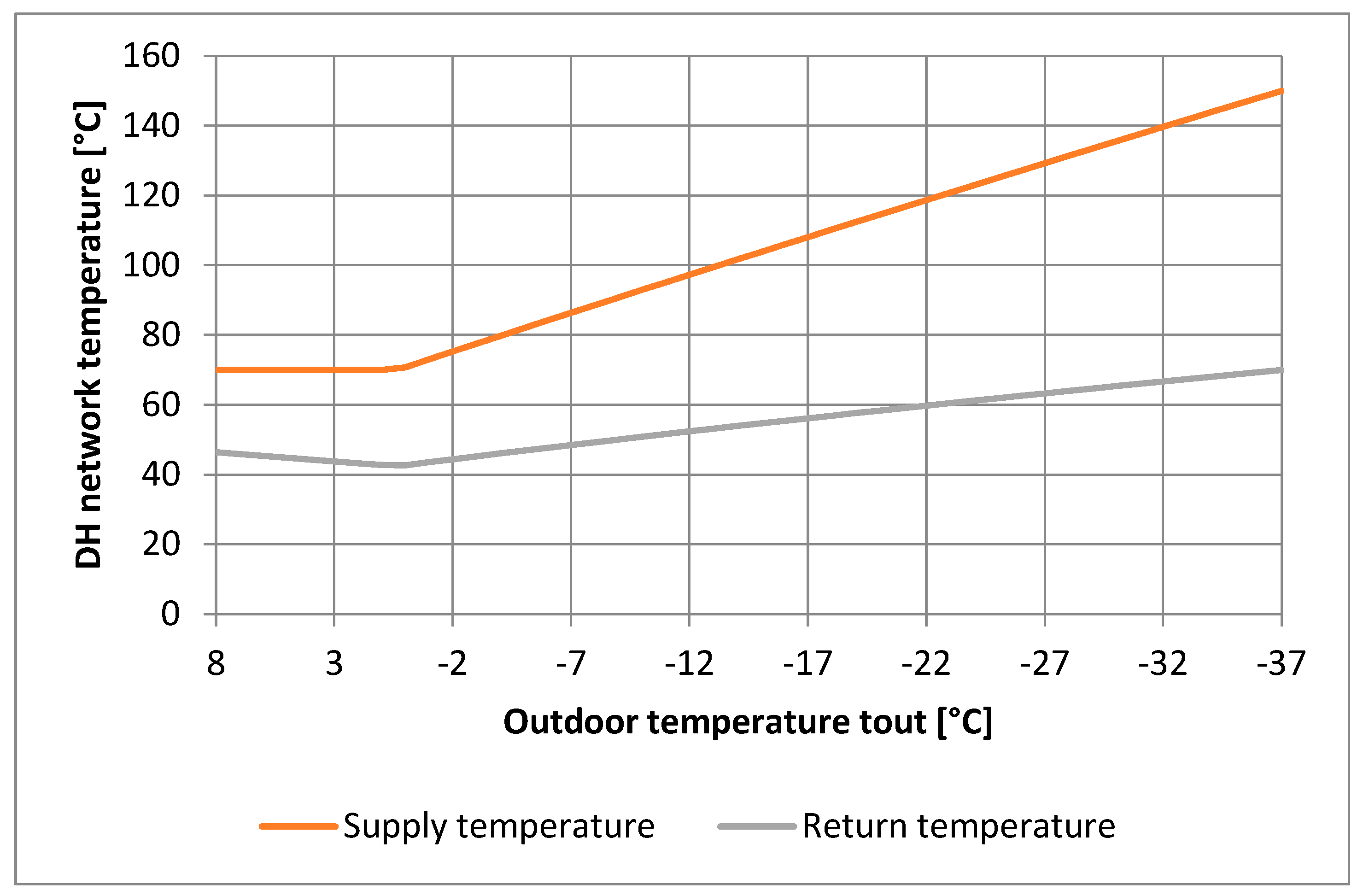
For most of the DH systems employing supply temperature control, the lowest supply temperature is a fixed value (
Figure 1).
The CPT indicates when the supply temperature should have dropped further due to the warm weather, but is still kept at 70 °C to ensure DHW service [
32], since, to some extent, the CPT was an uncertain parameter, with the corresponding value of the outdoor temperature set to +0.3 °C. To compare, in Norway, the same point is called CPT and has just an approximate value [
21]. According to ref. [
21], the value of the CPT indicates when energy consumption significantly decreases because of high outdoor temperature, but there is never zero SH heat demand.
2.3. Substation Configuration and Flow Control
To describe the thermal performance, the following general energy balance is applied for the hot water flow rate
(kg/s):
where
is the specific heat capacity of hot water.
This equation is used to relate measured flow rates and temperature differences to actual energy delivery, providing the basis for evaluating both substation efficiency and control performance.
To control the flow rate dynamically, especially when ambient outdoor temperatures change, the supply temperature setpoint is either manually configured or adjusted using weather-compensated control logic. The lowest supply temperature threshold is commonly maintained at around 70 °C to ensure stable delivery of DHW, even when SH demand is low. This strategy is illustrated in
Figure 1 and reflects common practices discussed in ref. [
21].
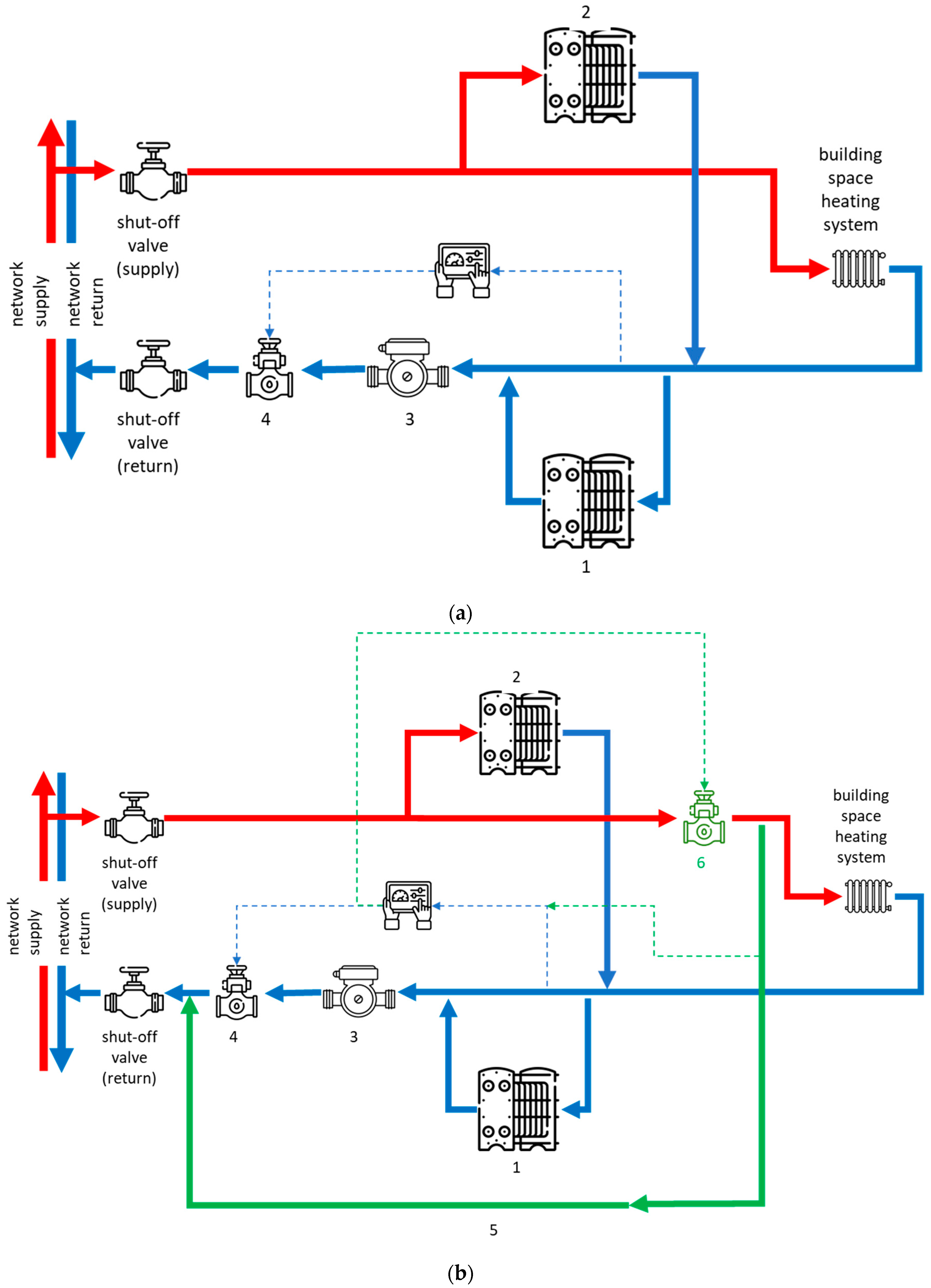
Figure 2 illustrates the physical layout before and after flow control improvements.
Here, each numbered component corresponds to a control or safety element. For instance, the self-acting temperature controllers (item number six) vary the flow of hot water through the secondary side based on outlet temperature readings. Differential pressure controllers (item number four in
Figure 2) ensure stable operation despite fluctuating building loads or network pressure changes. In the updated system (
Figure 2b), a bypass line has been added to enhance temperature control under low-demand conditions. The flow control is implemented through a combination of flow limiters, temperature sensors, and control valves, which interact to maintain desired temperature setpoints while preventing overheating or underflow.
A pump was used to ensure a differential pressure head, as it was not equipped with a variable-frequency drive (VFD). Excess heat was just damped into building envelopes, as substations do not adjust the temperature for each SH system. Now, temperature is additionally controlled with the help of an additional bypass line (
Figure 2b). Such control is often implemented by using a temperature sensor at the outlet of a group substation to adjust the speed of a pump. Similarly, the supply temperature is controlled to maintain a similar level regardless of daily varying heat consumption and is easily implemented with a short bypass line if needed.
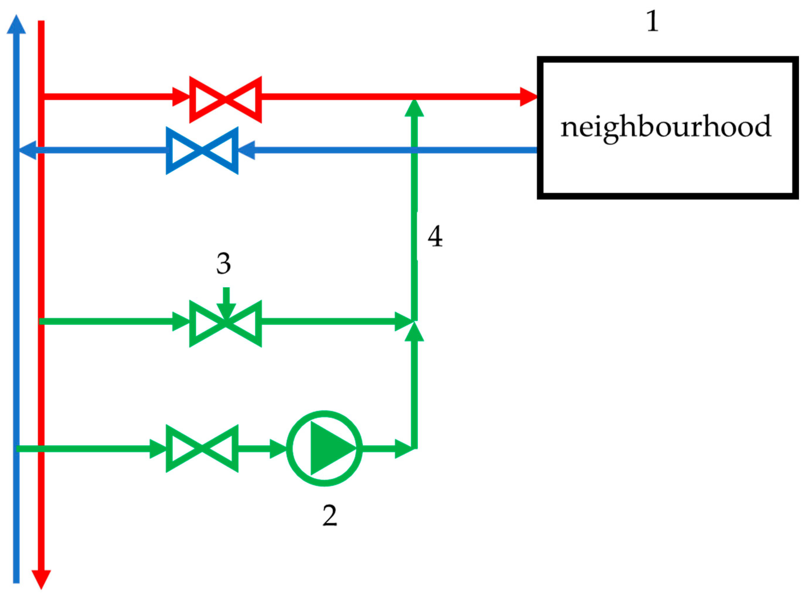
In networks without group substations, connecting components can be retrofitted. As shown in
Figure 3, a motorized temperature controller and VFD-equipped pump vary flow and temperature to match demand.
2.4. Group Substations
HTDH systems often employ group substations to serve a cluster of residential or mixed-use buildings, typically ranging from 5 to 15 units. These substations form the interface between the primary DH network and the secondary building-level distribution systems. Their purpose is to control and stabilize both thermal energy delivery and hydraulic performance across buildings with varying heating demands and architectural configurations.
A typical group substation includes one or more plate heat exchangers, differential pressure controllers, bypass valves, circulation pumps, and various flow- and temperature-control devices. The primary DH network supplies hot water at a preset temperature and pressure to the substation, where heat is transferred to the secondary circuit. The circulation pump, located on the secondary side, ensures a sufficient differential pressure head to maintain flow across the entire group of buildings. In systems where VFDs are not employed, the pump operates at a constant speed, and excess heat may be dissipated through building envelopes, leading to inefficiencies.
In systems lacking fine-grained control at individual buildings, the group substation often compensates by changing the entire cluster’s flow rate. When a VFD is not present, this is done by modulating a motorized valve in a short bypass loop (as in
Figure 3), responding to a sensor at the substation outlet. These control methods reduce pump energy use and avoid unnecessary overheating of the distribution circuit, while also contributing to demand-side efficiency.
Hence, a local distribution network after a group substation can run with a varying flow rate without allowing the supply temperature to increase excessively or decrease below the threshold required by the DHW system for its safe and stable operation.
Figure 4 presents the detailed schematic of the group substation, including filters, valves, and control elements.
2.5. Economic Assessment
The assessment of the network costs is described below. Typically, increasing the dimension also increases the capital expenditure, which includes purchasing the equipment, its installation, piping, and trenching:
where CapEx is capital expenditure, the total costs of the project [EUR];
IC is Initial Cost, i.e., the upfront cost of acquiring assets for a project [EUR];
ARR is Annual Recurring Revenue, i.e., the total expected revenue generated annually from a specific product, service, or asset [EUR];
OM is the annual operation and maintenance costs [EUR].
Trenching is the second largest component; its specific costs are assumed to be EUR 655/m for a pair of pipes 2 × DN400 or below and EUR 850/m for pipe dimensions 2 × DN400–800. In turn, capital expenditure is the primary factor affecting net present value (NPV).
where CFt is the annual net income at time step (year) t,
T is the life of investment,
i is the discount rate,
ICt is the cost of acquiring assets for a project at time step (year) t.
As relevant here, for a single pipe, trenching costs are EUR 100/m, which is apparently less than for the traditional double-pipe installation. To compare, Sommer et al. [
30] assume EUR 800/m if both supply/return lines DN400 and below are installed, and EUR 1000/m for larger pipe diameters. They set EUR 150/m for the single-pipe installation. As reported here, the cost of heat is assumed to change annually as a function of the inflation-adjusted cost of heat registered during the last month of the year.
Piping costs (including installation) are even greater, and the same with trenching. They vary according to the pipe diameter. Piping costs are set between EUR 55 and 355/m for a single pipe DN220–500; these values affect the payback period (PBP) significantly:
where CF is the total net income.
These cost estimates are based on actual market prices and are corroborated by [
33,
34].
As for the costs of the network, all the required elements are evaluated (including pipes, fittings, and joints), based on the relevant industrial sector investment guidebook and actual prices from the manufacturer. For the assessment given, the internal rate of return (IRR) should be positive (Equation (11)), even though piping assembly costs approximately 70–80% of the total price of pipes and fittings, which depends on pipe dimension, insulation type, and the number of elbows, anchors, etc.:
where i
1 and i
2 indicate the range, and where NPV becomes positive/negative; NPV
1 and NPV
2 NPV values are calculated for i
1 and i
2, respectively.
Operation and maintenance costs also vary, depending on network type; they also depend on i. They include pumping [
35], covering heat losses [
36], and service work [
37], including those of buried segments.
2.6. Environmental Performance and Emissions
To estimate emissions and fuel use, the boiler energy balance is used.
The maximum fuel saving and the associated abated CO
2 emissions of the DH system, controlled in another way with respect to the traditional operation, are obtained by evaluating the design consumption of coal burnt in a boiler unit to supply steam to a steam turbine of a CHP plant. Thus, thermal balance is
where B is primary energy consumption [kg/h];
LHV is lower heating value [kJ/kg];
ηKA is the efficiency of a boiler;
Gc is the hot water flow rate;
C is its density;
t1′ is the supply temperature;
t2″ is the return temperature;
ηm is the distributional heat losses.
Primary energy consumption [kg/h]:
Such a condition is achieved in correspondence with the design number of hours in which a CHP plant is operated in a CHP mode:
where q
4 is fly ash or coal combustion residuals (CCRs) losses.
Fly ash or coal combustion residuals (CCRs) [kg/h]:
where ash content
; and filter efficiency
.
By keeping the necessary amount of excess air and keeping constant the losses within a boiler, a maximum of Sulphur consumption is always achieved, as shown in Equation (16).
SO
2 production [kg/h] is:
where
and
are molecular masses of sulfur dioxide and Sulphur, respectively.
Carbon dioxyde production [kg/h]
where C
CO2 is CO
2 content in flue gas [g/m
3], V
g2 is flue gas rate at air ratio α set to 1 [m
3/kg], and V
g is actual flue gas rate [m
3/kg].
The configuration and control logic of the group substation directly influence the cost analysis and thermal balance calculations presented in later sections. For instance, a higher differential pressure head requires more pumping power and increases O and M expenditure, while ineffective temperature control can result in greater heat losses, affecting primary energy consumption (Equation (13)) and emissions (Equations (16)–(18)).
Furthermore, the configuration determines the heat load curve, which feeds into CapEx estimates and PBP analysis. The proper design and placement of substations, valves, and pumps must therefore be considered in any optimization of the DH network from both a hydraulic and economic perspective.
2.7. Simulation Environment
Thermohydraulic simulations before and after introducing group substations were performed in ZuluThermo© software, an add-on to ZuluGIS© (both Version 10.0.0.8075u). ZuluThermo© is a commercial simulation tool designed for hydraulic and thermal tuning of DH systems. One of its core features is the calculation of flow rates, which are essential for achieving optimal energy distribution and system efficiency. Flow rates depend on temperature difference, heat demand, control methods, and introduced scenarios. The last two items are non-numerical inputs.
The software calculates the required flow rates of heating medium based on the following two numerical inputs:
Temperature differences between supply and return pipelines (as described in
Section 2.2 DH Network Temperature Control).
Calculated thermal loads of individual consumers depending on outdoor temperature and system design parameters (as described in
Section 2.1 Heat Demand Modeling).
The software accounts for seasonal variations and extreme temperature conditions, ensuring the reliability of flow calculations under all operating scenarios. These temperature-dependent parameters are heat demand (see Equations (1)–(6)) and network temperatures (see
Figure 1 and Equation (7)).
The software supports both manual and automated control strategies at substations, including the following:
Direct connections, mixing (hydroelevator, see
Figure 5, or pump-based), and independent circuits.
Open and close DHW connections with one- or two-stage heating (see
Figure 2).
Simulation of substations with or without automatic control valves enables accurate modeling of partially or non-automated networks, as introduced below in the Case Study section. This flexibility allows users to model the influence of control valves, regulators, throttling orifices, and nozzles on system hydraulics and flow distribution. More details on ZuluThermo© software are available in ref. [
38].
3. Case Study
Omsk (Russia) DH system is considered to be HTDH. High supply and return temperatures in the networks result in high heat distribution losses and inefficient energy use, especially in fall and spring. Most of the residential districts and industrial facilities have already been connected to the existing DH system, because of the former USSR legislation, which used to promote DH technology over other methods of heat supply. However, according to the national regulation of that era, throttle devices such as hydroelevators (
Figure 5) or orifice flanges [
39] were prioritized over other methods of substation connection.
New energy-efficient buildings typically contain a DH substation incorporating a pump and a branched SH system with floor heating. These buildings do not necessarily constitute new neighborhoods; they can be easily integrated into existing urban infrastructure. Several such meshed districts are being built in Omsk, which exacerbates the hydraulic balance of the DH network. As supported by Volkova et al. [
4], it is possible to reconfigure these districts so they can operate with lower supply temperatures. That entails modernizing a group substation according to the Materials and Methods section and/or constructing new sections of a DH network so buildings within these districts can form an LTDH area. A similar situation of meshed new and old buildings is reported in Estonia [
4], Croatia [
40], Denmark [
41], France [
12], etc. The legacy of the USSR is a high share of CHP-based energy production, suffering especially severely from high return temperature. Similar to plenty of cities and towns in former CIS countries, in Omsk, the source of energy is a CHP plant firing coal. Its Sulphur content
.
The heat demand for the model relevant for 2022 is defined by the operational data of 2021, with an annual increase of design heat demand by 0.9% (new consumers to be connected in 2022), but a similar monthly distribution. Supply and return temperatures vary across the year’s seasons, with the declared regime of 150/70 °C (peak supply/peak return). However, due to the poor condition of the DH network, the maximum supply temperature is 110 °C, which corresponds to the outdoor temperature of −28 °C and below (
Figure 6).
That results in an average error of the hourly forecasted heat demand of 17.3%. To compare, in Kristensen et al. [
22], a mean absolute percentage error of the hourly forecasted energy consumption of 11.8%. In addition to the coldest winter days, in Omsk, the fall and spring months (outlined in red) are the major contributors to the total heat demand forecast error; now, an advanced model with the additional variable of flow rate is applied. The lowest accuracy occurs outside of the Danish SH season (starting in October and ending in April); the performance is especially poor during the coldest winter days when predictions were, on average, 23.5% higher than the values recorded.
With a monthly average supply temperature of 77.2 °C, the summer season period is abnormal. The supply temperature is much higher than required to cover DHW demand over the summer of 2021. The reason for keeping it so high is the CHP plant’s electricity generation plan.
Due to the same reason, it is also higher than needed during the fall and spring months, e.g., November 2021 (
Figure 7).
With an ordinary configuration of a substation (
Figure 2a), all this excessive supply temperature is delivered right to the building substation.
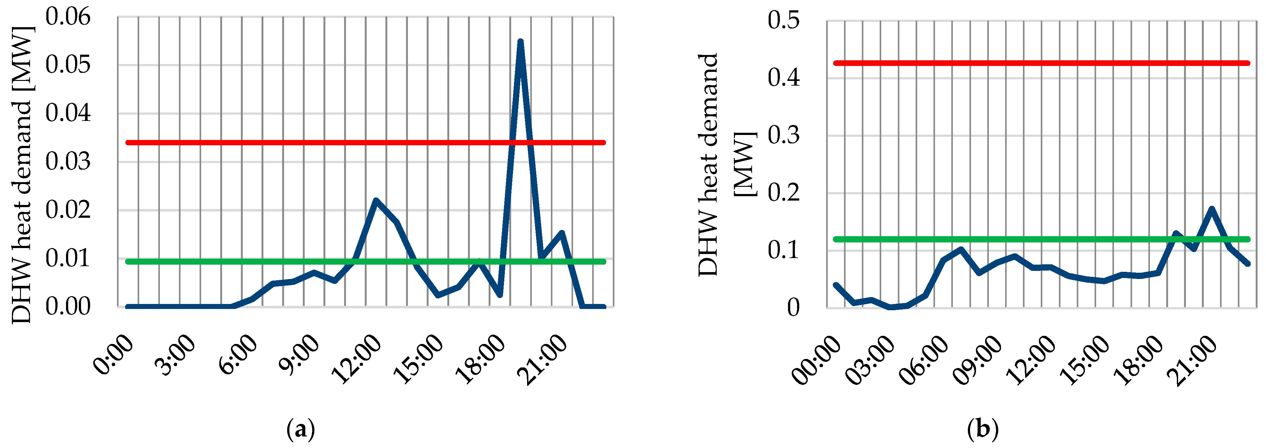
Total heat demand consists of SH and DHW components. While SH with a proper accuracy can be modeled with the help of linear equations as Equations (1)–(6), the DHW component has highly stochastic and non-linear behavior as presented in
Figure 8.
The actual recordings from a heat meter showed that over a typical day, the SH contributed to 75% of the total energy consumption, and 25% was related to DHW. For an office building (
Figure 8b), DHW is responsible only for 11% of the daily heat demand, while 89% is associated with SH. These profiles represent the situation of allowing all the surplus energy to be dumped into the building envelopes and all the surplus to increase the indoor temperature. To compare, Ivanko et al.’s [
21] observations point out that the SH contributed to 75% of the total heat use over the studied year, while the remaining 25% was related to DHW. When the outdoor temperature is 0.3 °C and above, the supply temperature is still 70 °C. That means an outdoor temperature of 0.3 °C is CPT; for this temperature and above, SH constitutes as much as 79% of the total energy consumption, while 21% is associated with DHW use. According to
Figure 7b, the indoor temperature is significantly higher than the design value of 20 °C in buildings whose SH systems are connected to the substations with no active flow rate control but equipped with throttle devices only (orifice flanges and hydroelevators). This share of the energy demand is treated as overconsumption. To compare, in Ivanko et al. [
21], SH was responsible only for 7% of the heat used in a temperature range above the CPT, while 93% was associated with DHW.
Due to the unpredictable behavior of the DHW component (see
Figure 8) and its relatively high share (up to 25%), only the operational data can be used to ensure the proper accuracy of the simulations when considering a residential neighborhood. Therefore, operational data for a certain neighborhood were used when calculating total flow rates. The analyzed case study is situated in a residential district characterized by mid-rise apartment blocks, located between Mayakovskogo Street and Potanina Street. The DH network in this area serves a cluster of multi-family buildings, interconnected through a combination of above-ground and buried pipelines.
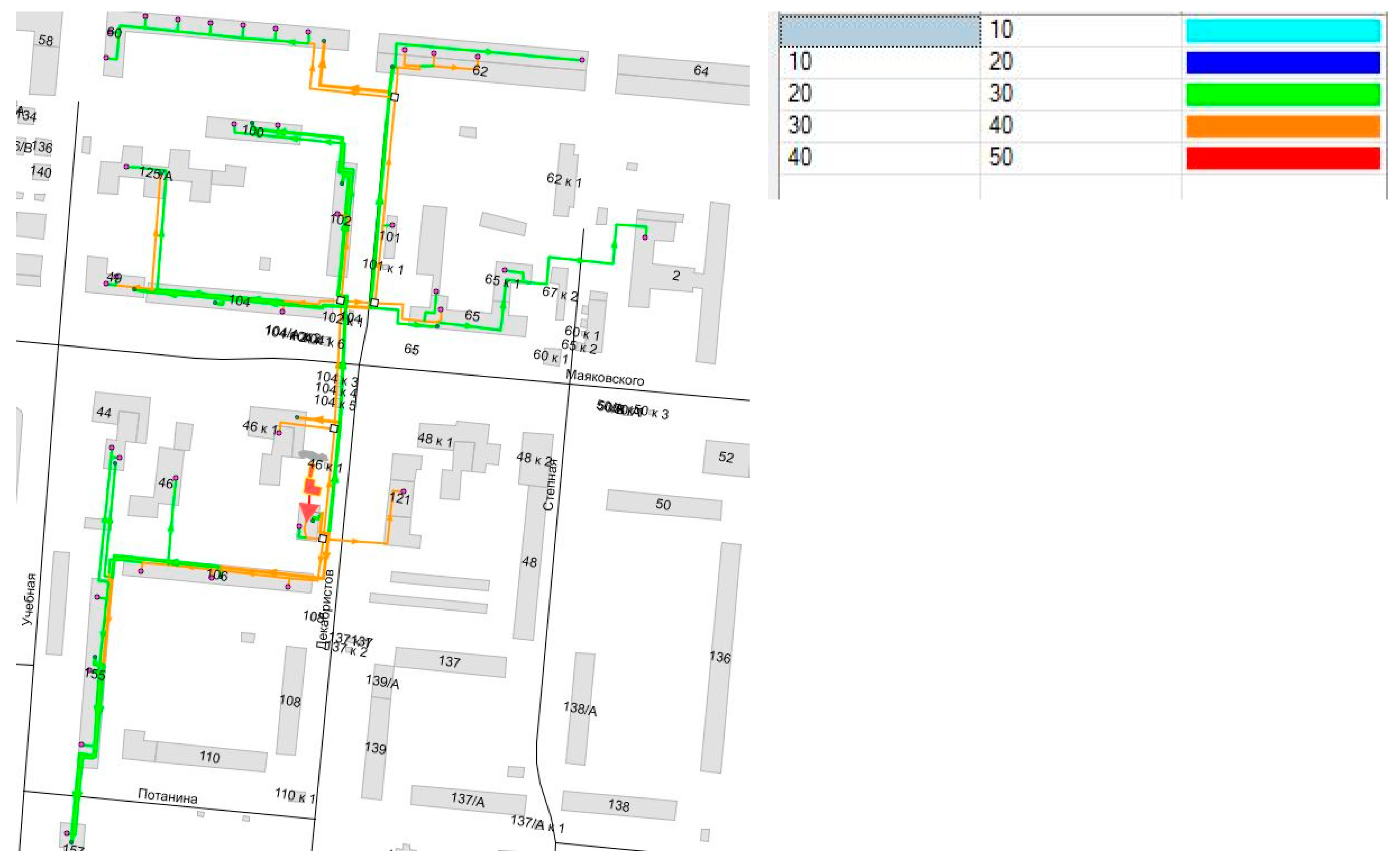
Figure 9 illustrates the DH network layout, where the main supply and return pipelines are clearly marked in green and orange, respectively.
The network features several branches, each delivering thermal energy to multiple building entrances. The central node, located near building 46 on Mayakovskogo Street, appears to act as a group substation or a major distribution point. This node connects to secondary branches that distribute heat to nearby buildings such as 46k1, 104k1, and 48k1. The system serves a significant number of buildings, ranging from older housing units to more recently constructed apartment blocks, indicated by varying pipeline lengths and diameters.
Flow control elements, including differential pressure controllers, pumps, and bypass lines, are strategically located along the network to maintain thermal and hydraulic balance. The network operates under outdoor temperature-compensated control logic, particularly relevant given the area’s varying seasonal heat demands. This case study provides a representative example of urban-scale DH deployment where control strategies, such as bypass installation and group substations, significantly influence operational efficiency and temperature regulation.
Apparently, shared pipe sections unite the flow rate to several substations. The orange color represents sections of the DH network with volumetric flow rates ranging from 20 to 30 m
3/h, green at 30 m
3/h or lower, and red over 40 m
3/h. The average daily flow rate is defined using hourly profiles for a typical winter day for a residential and an office building, given evenly distributed hourly SH and actual DHW demand profiles (
Figure 8a,b). Excessive energy generation is detected when the energy produced exceeds the sum of energy consumed to ensure an indoor temperature of 20 °C and cover distribution heat losses (
Figure 10).
The cold season model of operation remains the same without any change. The reason is that we focus on each single substation response only when the return temperature is higher than it should be, and when overheating is registered. Hence, there is no need to assess the thermal behavior during winter and summer, especially the former, when the supply temperature is often lower than it should be. For fall and spring, before starting the forecast calculation, the algorithm checks if the outdoor temperature is below +0.3 °C and the supply temperature is 70 °C and above, and if both conditions are fulfilled, the winter season model is used to deliver energy into a district—the bypass line model is used. Moreover, before moving any valve actuators, the algorithm checks if there are any local DHW exchangers (rare conditions, only if an existing third DHW pipe is out of service), and if so, the winter season model runs anyway; otherwise, again, the new configuration is applied.
At a full winter demand, all the pumps at a group substation run with no bypass line, and the valves in the group substation conduits are fully open. As the heat demand decreases and outdoor temperature increases, the temperature sensors in front of the third pipe start to open their valve, simultaneously limiting the flow rate through the main supply line.
Modeling conditions are as of the typical fall/spring day of an outdoor temperature of 2 °C, but with a new design of a group substation, a maximum (not minimum anymore) supply temperature after a group substation set to 70 °C, and a mixing pump running.
The measurement and operational data used in this study were collected from a real-life DH system over two full years, spanning from 1 January 2020 to 31 December 2021. Data were obtained at one-hour intervals using calibrated automation sensors installed within the central DH plant, group substations, and selected building substations. Supply and return water temperatures were measured using Pt100 resistance temperature detectors with an accuracy of at least ±1 °C. Flow rates were recorded using ultrasonic flow meters with an accuracy of at least ±1.5% of the measured value. DHW consumption was tracked via ultrasonic water meters installed at the substation outlets with an accuracy of at least ±1 °C. Due to the wide variety of models and manufacturers, only the upper threshold values for installed sensors are reported here. Both supply and return temperatures and flow rates at primary and secondary sides, as well as DHW readings, were available.
As mentioned above, the meters and temperature sensors are installed at
DH plant outlets,
group DH substations (indicated as a red triangle for this case study), and
particular individual substations.
The exact location of the individual substation where measured data were available cannot be disclosed due to privacy and GDPR reasons, as it can trace back to billing procedures and occupants’ behavior (e.g., office hours, waking up, and returning home time).
All simulation outputs were calibrated using the collected hourly temperature and flow data, along with indoor room temperature measurements. Calibration quality was assessed following ASHRAE Guideline 14-2014. The coefficient of variation of the root mean square error (CV-RMSE) for the indoor temperature model was calculated at 9.3%, and the normalized mean bias error (NMBE) was −4.1%, both within the acceptable thresholds of 15% and ±5%, respectively, for hourly data. These error metrics confirm the model’s adequacy for simulating the thermal behavior of the buildings and DH system under the observed operational control regime.
4. Results and Discussion
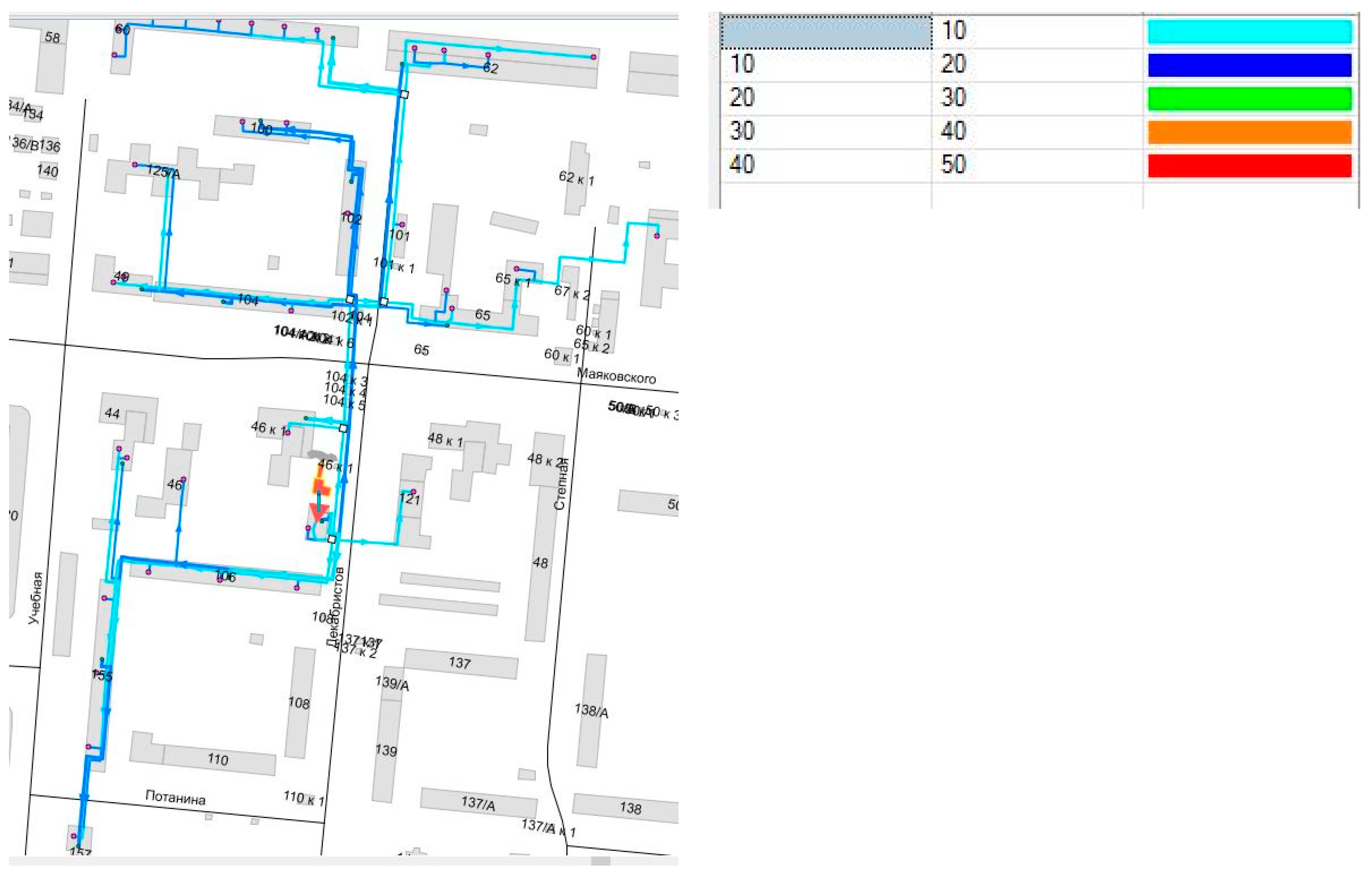
Figure 11 presents the modeling results of the same subsection of the DH system.
Flow rates are now mostly depicted in somber colors, associated with figures of 20 m
3/h and below. Please note an interesting result of the DH network simulation: the section running through building #155 is depicted in light blue, while more remote/distant sections of the distribution network are depicted in blue, representing energy saving. The reason is that the redistributing flows of hot water are just around 10 m
3/h due to the high DHW consumption of the second substation of building number 155. Overall, the novel configuration determined by the variable flow rate is capable of achieving the primary objective of the research, which was to shave supply temperature by exploiting the local potential of network control without decreasing the indoor temperature. To compare, in ref. [
14], the optimal regulation characteristics determined by the model predictive control were able to fulfill the primary aim of the paper, which was to cut the peaks of the heat demand profile by utilizing the accumulating ability of the envelopes, again, keeping the indoor comfort intact.
Therefore, because of the slightly lower supply temperature and less energy delivered, a lower return temperature is expected, which is a similar behavior to most of the buildings in Omsk and was observed in 73% of the studied buildings. To compare, in ref. [
19], the high-temperature difference is the opposite behavior to the buildings in Gothenburg, Sweden, and was detected in 26% of the studied substations. These district cooling substations are characterized by a return temperature of 10–15 °C and the potential to achieve even higher return temperatures (opposite to generally beneficial lower return temperatures in DH).
Now, the flow sensor at the supply line coming from a DH plant (
Figure 3, unit number three) detects the temperature increase and increases flow from a return line by opening the bypass pipe (
Figure 3, unit number four) and/or running a pump (
Figure 3, unit number two) to maintain a lower temperature, but additional flow in the supply line. Energy demand accurately changes with outdoor temperature increase or decrease; operation of a pump equipped with a VFD also follows operational data, namely hourly and daily variation of flow rate, which, in turn, depends on many factors, e.g., whether it is a weekday or a weekend [
42]. Implementing the proposed scheme in the real world requires monitoring flow rates and temperatures obtained by manual checking and visual observation. A more advanced solution is also easy to imagine; data for this can be acquired by a low-cost remote control already available on the market. An outdoor temperature sensor is also required, while recordings from a heat meter are necessary to check actual energy consumption and other factors, e.g., solar radiation. Alternatively, the SCADA system or the local provider of DH services may provide this data.
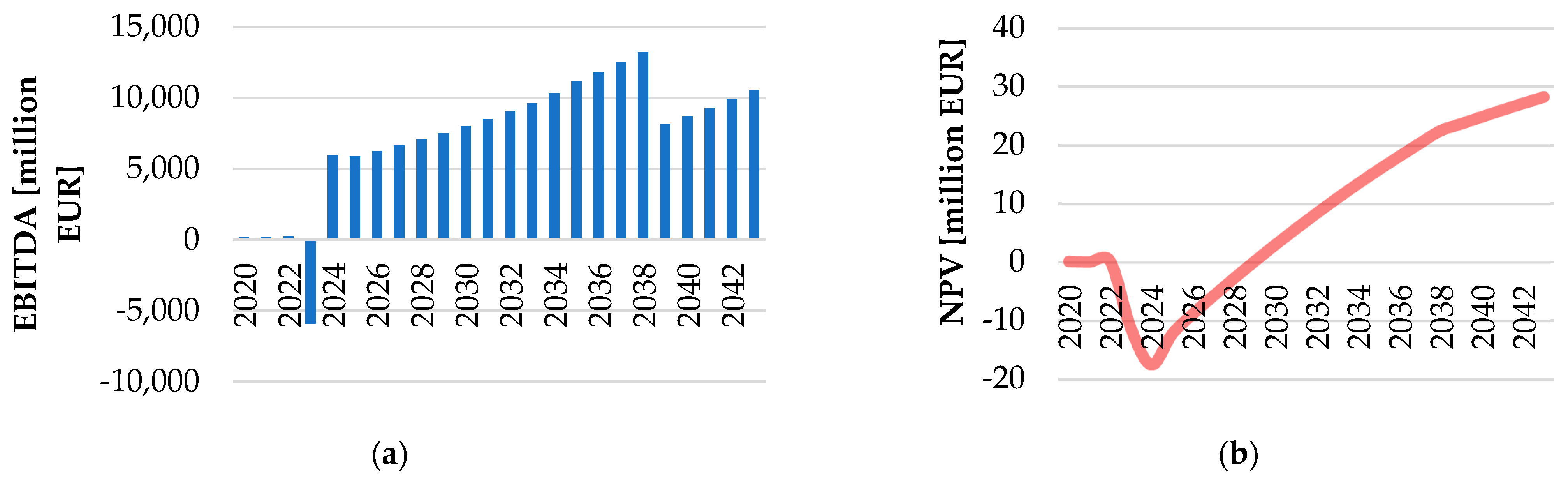
Eventually, a feasibility study is underway that implies obtaining the annualized costs of the new typology. The lowest total lifetime cost occurs at an annual average supply temperature of 78 °C and an average annual outdoor temperature of 8 °C, while IRR is 25.4% (
Figure 12).
Assuming the optimal operation for the lower temperatures and design characteristics of the components of the scenario are characterized by higher exergy efficiency, this is a promising result as the minimum waste of heat (both demand and distribution sides) occurs at the lowest supply temperature at the operational stage. From
Figure 12b, the total cumulative NPV of the project becomes positive in the ninth year with an average supply temperature of 70 °C for relative values of high outdoor temperature. To compare, Harney et al. [
26] report the optimum network configuration for lower temperatures since the lifetime cost of distribution losses, electricity consumption, substations, and piping is minimized. This is a satisfactory result since the minimum cost of each parameter is related to different design temperatures for the same optimum layout. According to the three tables provided in ref. [
26], the lowest costs are achieved at a supply/return temperature difference of 27 °C.
The economic performance here mostly depends on the capital costs. In the advanced heat supply scenario, the total earnings before the deduction of interest, taxes, depreciation, and amortization (EBITDA) for the DH system are EUR 25,300 (if no group substation has been installed). EBITDA for the already prepared system (pipe material for a bypass line and hydraulic pumps only) is lower and accounts for EUR 13,900 (55% of reference costs). The common advantage of the new supply scenario is that no cost- or labor-intensive modernizing of the DH network is required. To compare, in ref. [
4], the necessary additional capital costs are about EUR 66,000, which is 16% more than the capital costs associated with the baseline scenario. Wirtz et al. [
9] suppose generating energy with PV only, with the total expenses of EUR 84,500/a (13% of TAC), are the costs for PV modules.
Because of the piping and fitting, capital costs are higher than for the reference option. However, almost no costs are required for a central station (except for a bypass line), and no expensive heat exchangers decrease costs when compared to the energy cascade three-pipe option [
4]. The necessary additional capital costs are about EUR 12,860, which is 49% more than the investments required for continuing working ‘as is’ (refer to
Figure 12a).
The highest negative EBITDA (about EUR 56.0/MWh) is EUR −5915, achieved in 2023. Total EBITDA is EUR 174,800. To compare, in ref. [
15], for a very high cost of heat (EUR 66.0/MWh), a decrease in primary energy savings is detected because of the significant period of running the auxiliary gas-fired heater. Since similar technologies but different components in ref. [
4,
6,
30] are considered, operation and maintenance costs and investments are hard to compare.
Operation and maintenance costs are considered by evaluating heat loss, pumping power, and servicing heat exchangers, valves, and pipes. To compare, Sommer et al. [
30] consider electric energy demand only, explaining that maintenance costs for any network topology are similar.
The regular operation has operation and maintenance costs of EUR 411,000, while the optimized operation results in EUR 183,000, which makes the costs EUR 227,000 lower. To compare, Hering et al. [
27] report negligible operation and maintenance costs for the rule-based operation of EUR 638, while for the optimized operation, they account for even less, EUR 603, or a 5.49% decrease in cost.
For the case study conditions, annualized costs are EUR 16,400 and 7340 for the reference and for a new type of operation, respectively. As for the latter, the values are obtained assuming the 25-year life span of the main components, which results in an annual saving of 55.3%. The primary reason for savings is the decreased heat consumption of the optimized operation compared to the traditional operation. This thermal load reduction is mainly achieved with a lower heat demand during warm fall and spring days.
The great importance of annual energy consumption in the interest of one or another scenario is also demonstrated in refs. [
27,
28]. In ref. [
31], even some scenarios implying supply temperatures of 105/55 °C, 100/50 °C, and 95/50 °C are only beneficial if energy consumption is somehow decreased by 20%. Here, it is demonstrated by
Figure 6, which illustrates the historical supply temperature over 70 °C during moderate-cold days and an excessive amount of heat actually delivered.
In ref. [
28], annualized costs for booster heat pumps, ranging between EUR 11,700 and 10,800, are derived during the 30-year life cycle of the systems, meaning an annual saving of 7.7%. According to
Figure 12b, the annualized cash flows range between EUR 5790 and 10,600/year for heat loss, pumping power, and EUR −9030–15,900/year for installing heat exchangers and piping. To compare, for a bidirectional low-temperature network, the annualized costs for the elements of a DH system were EUR 147,000/year (40% of total annualized costs) and others of EUR 94,100/year (25% of total annualized costs) [
9].
Under the assumptions followed, the advanced type of control shows better results than the reference scenario for the design energy consumption of 11.7 MWh. The results show that the transition from the current temperature regulation in Omsk to the flexible supply flow rate is a promising solution due to positive NPV. To compare, Romanov et al. [
31] consider 105/50 and 110/55 °C temperature regimes as less preferable. However, they take them into account if energy-conservation measures are implemented on the demand side to decrease heat demand by 5, 10, or 20%.
Direct GHG emissions are calculated with the help of Equations (12)–(19) that take into account the energy losses to induce mechanical circulation of hot water, electricity pumping (or fans in flue gas suction, ηKA), and additional heat demand to cover heat losses (ηm).
The results of the NO
x, SO
2, and CO
2 emissions reduction calculations are displayed in
Table 1.
In a novel configuration with an increase of 17% efficiency, direct CO
2 emission is 6.12 kg CO
2/kWh of heating (0.005 kg SO
2/kWh). For a reference case, it was 7.85 kg CO
2/kWh of heat. This reduction is equivalent to the annual GHG emissions from 306 passenger cars and the generation of electricity for 154 average single-family houses. To compare, Kilkis et al. [
29] consider switching to boilers with 0.83 kg CO
2/kWh of heat, which is lower than the direct CO
2 emission of 1.43 kg CO
2/kWh in the case of utilizing existing stoves. They evaluate efficiency at 0.35. Another difference is their methodology that ignores the energy losses during thermo-mechanical circulation of heating fluid, pumping, electricity demand, etc., hampering development and the achievement of a common base with other papers.
The externally supplied energy in both Sommer et al.’s [
30] and our paper is about electricity from the power network. Considering CO
2 emissions associated with one kWh of energy for pumping, the CO
2 impact is supplemented. However, Sommer et al. [
30] do not undertake any evaluation in this matter since they only considered the seasonal patterns of electric energy consumption, which do not vary significantly. An amount of 3168 CO
2eq tons/year of additional emissions was obtained in this paper. The largest effect corresponds with the new flow rate and temperature regime when they easily change and account for 6537 t CO
2. To compare, Romanov et al. [
31] present the largest absolute values corresponding with the 95/50 °C temperature regime, resulting in 1325–1387 kt CO
2 of annual emissions.
Because of high NPV and environmental indicators, advanced control of a DH system with a focus on operational data seems credible as it envisages 15,909 t of CO
2eq emissions and implies relatively low costs to avoid these emissions (EUR 1.59/tCO
2 per year, EUR 25,280 divided by 15,909 t of CO
2eq emissions). Data described in ref. [
4,
6,
43] corroborate the thesis that the high technology costs do not necessarily imply high costs of avoided CO
2 emissions. Regardless of the long payback period, Ziemele et al. [
6] found the best scenario, which envisages a 78.1% reduction in CO
2 emissions and relatively low costs to avoid these emissions (EUR 10.4/tCO
2 per year). The difference in electric energy demand in our paper and Ziemele et al.’s paper [
6] results in a significant difference in CH
4 impact due to electricity generation at CHPP number three, which is fed by natural gas. However, besides the high exergy efficiency indicator, our suggestion still reduces GHG emissions, while the costs to avoid emissions are also lower.
The main issue is the lack of any government program that limits GHG emissions at the heat distribution stage. DH mostly provides services in residential areas, where occupants live in multi-story buildings, so the demand for emission-free heat is low. Kleinertz et al. [
24] give another reason for tenants consuming heat while the landlord decides on the heat supply technology, but conclude the same—no public incentives for new technologies. Moreover, inhabitants typically consume energy for domestic purposes, while local authorities, supported by industry and government, are in charge of any strategic decisions. Although their local boilers (mainly firing natural gas) and heat exchangers have negligible ozone depletion potential, they are indirectly responsible for additional barriers to implementing technologies of a sustainable future (refer to ref. [
29] as well). Another factor accelerating the development of a viable control strategy is the low heat demand of individual large-scale customers, mainly industrial sites, and their call for emission-free district energy to reduce ecological fines and payments.
The idea is to install a bypass line to regulate supply temperature and flow rate to buildings located in one particular subnetwork after a group substation, bringing the levelized cost of heat (LCOH) value to EUR 51.6/MWh, which is 17.2% higher than in the reference scenario, along with a payback period of 10.0 years. To compare, in ref. [
6], the solution of introducing a low-temperature branch to houses situated in the low heat density area gives a higher LCOH value of EUR 35.21/MWh, which is 46.5% lower than here, and the payback period is 3.8 years. The difference is that there is no low heat density area, high distribution losses, and expensive equipment, piping, and components due to currency exchange. As for correlation with heat demand and sensitivity analysis, the initial number of consumers may be increased by decreasing the cost of energy. Moreover, combined economic, environmental, and social gains may exceed the investment required by modernizing a group substation, making it even more profitable for higher energy consumption values. However, sensitivity analyses show that the CO
2 emissions reduction is decreased by 4.5%, 7.2%, and 11.9% in the case of a 5%, 10%, and 15% reduction of the energy consumption of buildings, respectively, compared to the reference case. A similar conclusion is clearly visible in ref. [
15] where the primary energy consumption and the CO
2 emissions of the auxiliary gas-fired heater are reported to correlate with the number of DH consumers. In ref. [
6], another concept that involves large investments in PV panels, booster heat pumps, and central heat pump is described. It increases the value of LCOH by 21.6% and the payback period to 12.3 years, making it less feasible from the business perspective. To compare, Romanov et al. [
31] present the CO
2 emissions reduction by 1–2%, 3–5%, and 5–8% in case of a 5, 10, and 20% decrease in the energy consumption of buildings regarding the baseline scenario, respectively.


