

Power Production, Inter- and Intra-Array Wake Losses from the U.S. East Coast Offshore Wind Energy Lease Areas


Abstract
1. Introduction
1.1. Growth of Offshore Wind Energy Installed Capacity
1.2. Trends in Offshore Wind Energy
1.3. Wind Turbine Wakes in and from Offshore Wind Farms
1.4. Objectives
- To quantify likely power production from offshore wind energy lease areas along the U.S. east coast and how power production efficiency varies across a range of plausible installed capacity densities (ICDs) and between two widely used wind farm parameterizations.
- To quantify whole wind farm wake extents and power losses due to both internal and external wakes and how they scale with ICD. We further quantify the likely effect from wakes generated by the ‘second-generation’ of lease areas along the U.S. east coast on the ‘first-generation’ lease areas in which wind farms are currently being developed.
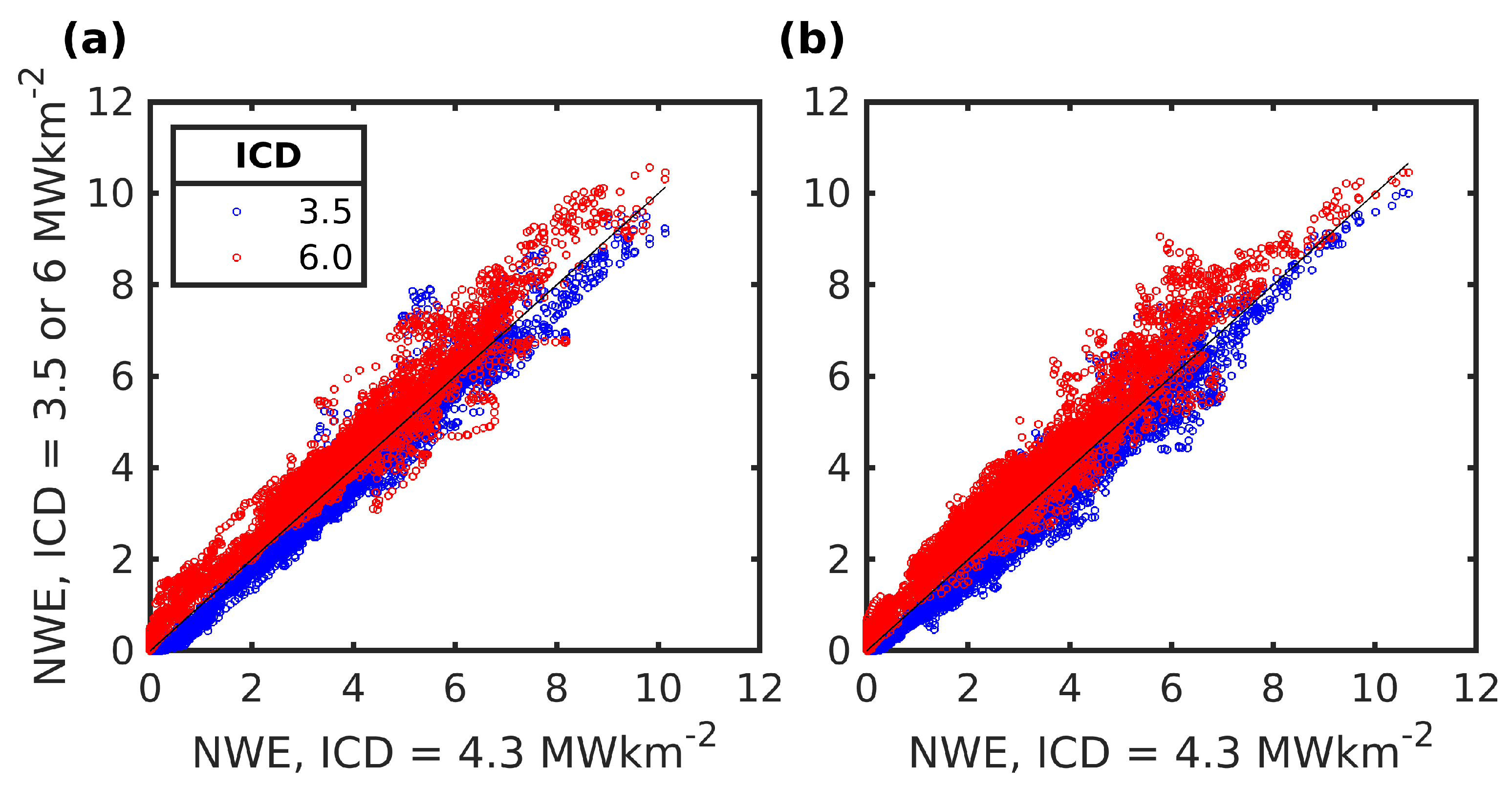
- To examine the dependence of projected power output from the largest wind energy cluster (3675 km2) on ICD (3.5 to 6 MWkm−2) in the context of previous research on wind power density limits.
2. Materials and Methods
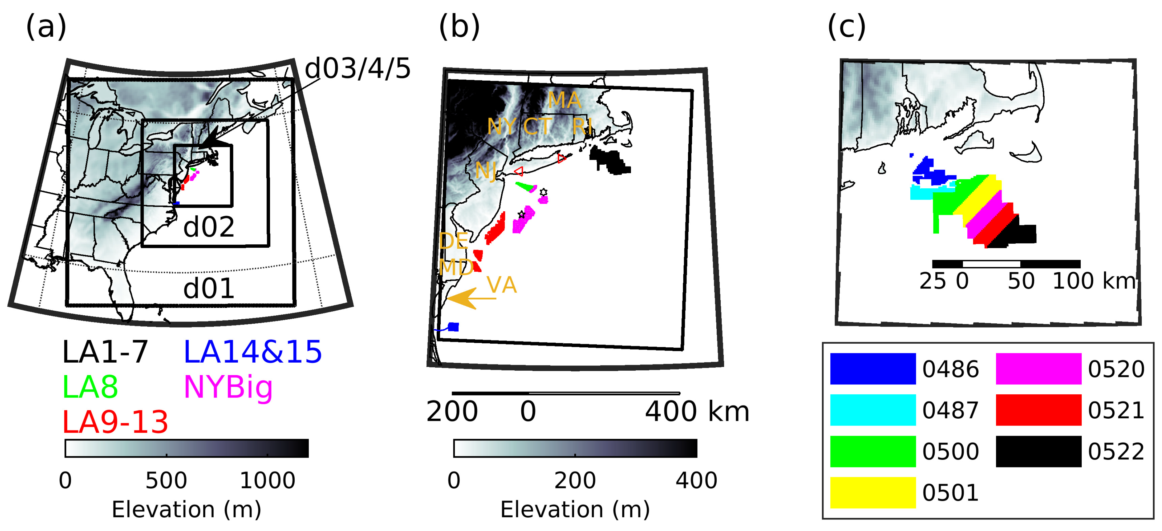
2.1. Simulations
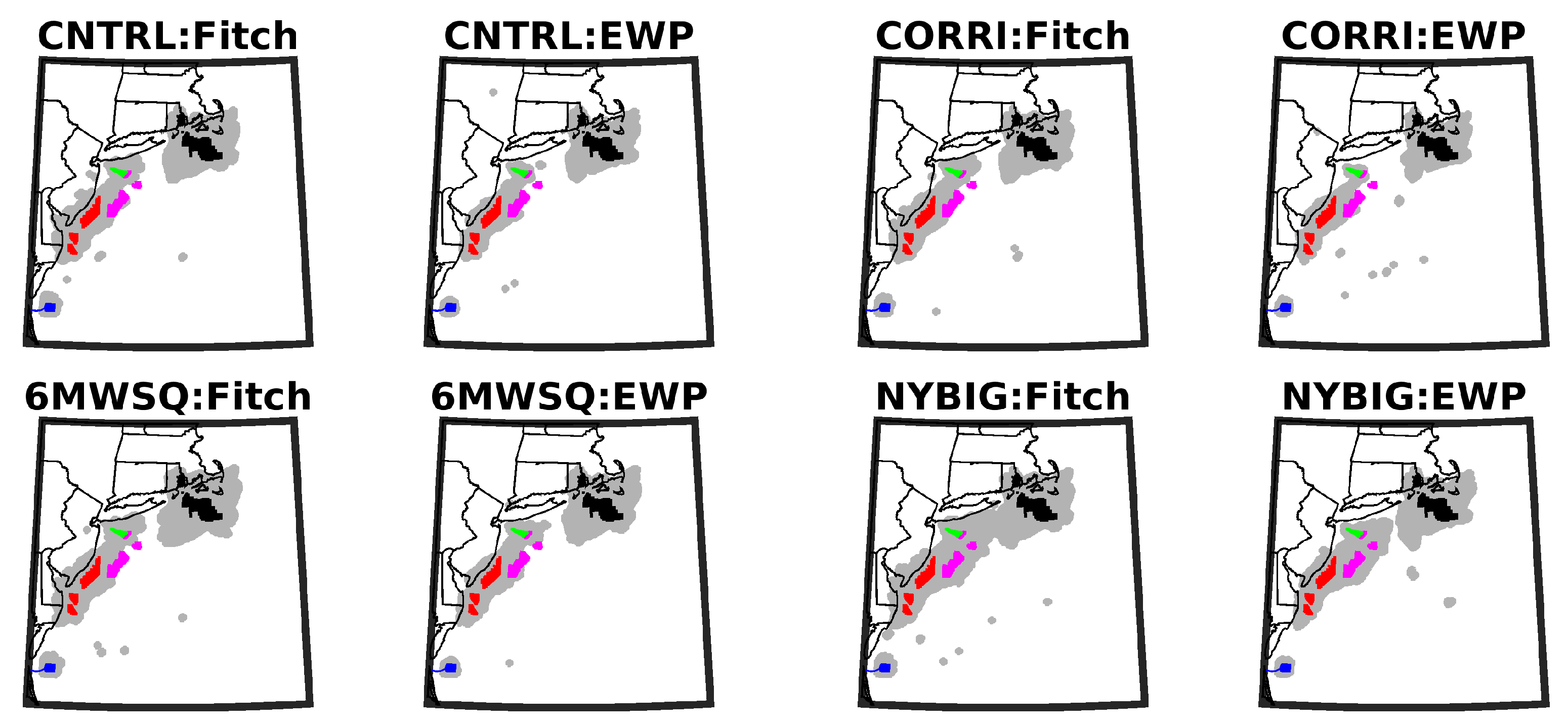
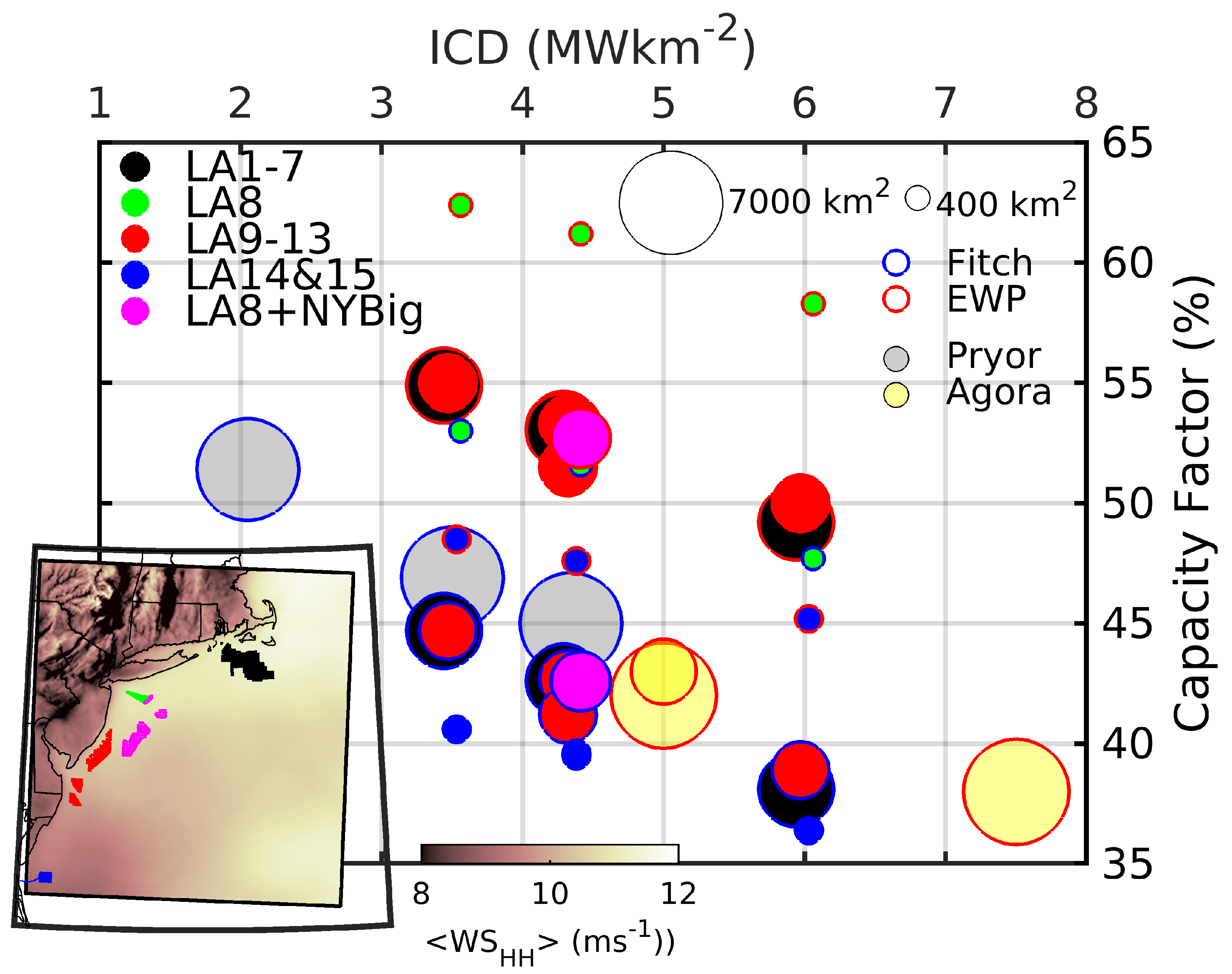
- LA1–7 (OCS-A 0486, 0487, 0500, 0501, 0520, 0521, 0522) collectively cover 3675 km2 and are south of Massachusetts (MA) and Rhode Island (RI).
- LA8 (OCS-A 0512) is located off the coast of New York (NY), south of Long Island, and covers 321 km2.
- LA9–13 cover a total area of 2105 km2 and lie east of New Jersey (NJ) (OCS-A 0499 and 0498), Delaware (DE) (OCS-A 0482 and 0519) and Maryland (MD) (OCS-A 0490).
- LA14 and 15 (OCS-A 0483 and 0497) cover an area of 465 km2 and are located east of Virginia (VA).

| Layout | d01 | d02 | d03/04/05 |
|---|---|---|---|
| Grid spacing (dx in km) | 16.67 | 5.56 | 1.85/1.85/1.85 |
| Wind farm parameterization | - | - | -/Fitch/EWP |
| Longwave radiation | Rapid radiative transfer model (RRTM) [76] | ||
| Shortwave radiation | Dudhia [77] | ||
| Microphysics scheme | Eta [78] | ||
| Cumulus scheme | Kain–Fritsch [79] | -/-/- | |
| Surface layer | MM5 similarity [80] | ||
| Land surface model | Noah [81] | ||
| PBL scheme | Mellor–Yamada–Nakanishi–Niino 2.5 (MYNN2.5) [82] | ||
- CNTRL: Wind turbines are deployed on a regular grid separated by 1.85 km in LA1–15. For the 15 MW wind turbine considered herein this spacing results in a mean ICD ~4.3 MWkm−2, and it equates to a separation distance of ~7.7 D which is approximately the mean value for operating offshore wind farms in Europe [27].
- CORRI: Wind turbines are deployed on a regular grid separated by 1.85 km in LA1–15 (as in CNTRL) but every sixth north–south row is removed to generate marine corridors. The resulting mean ICD is ~3.5 MWkm−2. Based on publicly available data, the world’s largest offshore wind project, Hornsea 1 and 2, have a similar average ICD of ~3 MWkm−2.
- 6MWSQ: Wind turbines are deployed at a higher density in LA1–15 for a mean ICD ~6 MWkm−2 and an average separation distance of ~1.6 km (~6.7 D). This ICD is similar to that of the Rødsand offshore wind farm in Denmark that covers 35 km2. It is also an ICD scenario considered in the Agora study of possible offshore wind energy expansion in the German Bight [84].
- NYBIG: Wind turbines are deployed as in the CNTRL layout for all of the ‘first-generation’ LAs plus those auctioned in the New York Bight (NYBig) in February 2022. As in CNTRL the mean ICD is ~4.3 MWkm−2.
2.2. Data Analyses
3. Results
3.1. Power Production, Capacity Factors and Efficiency
3.2. Wake Extents
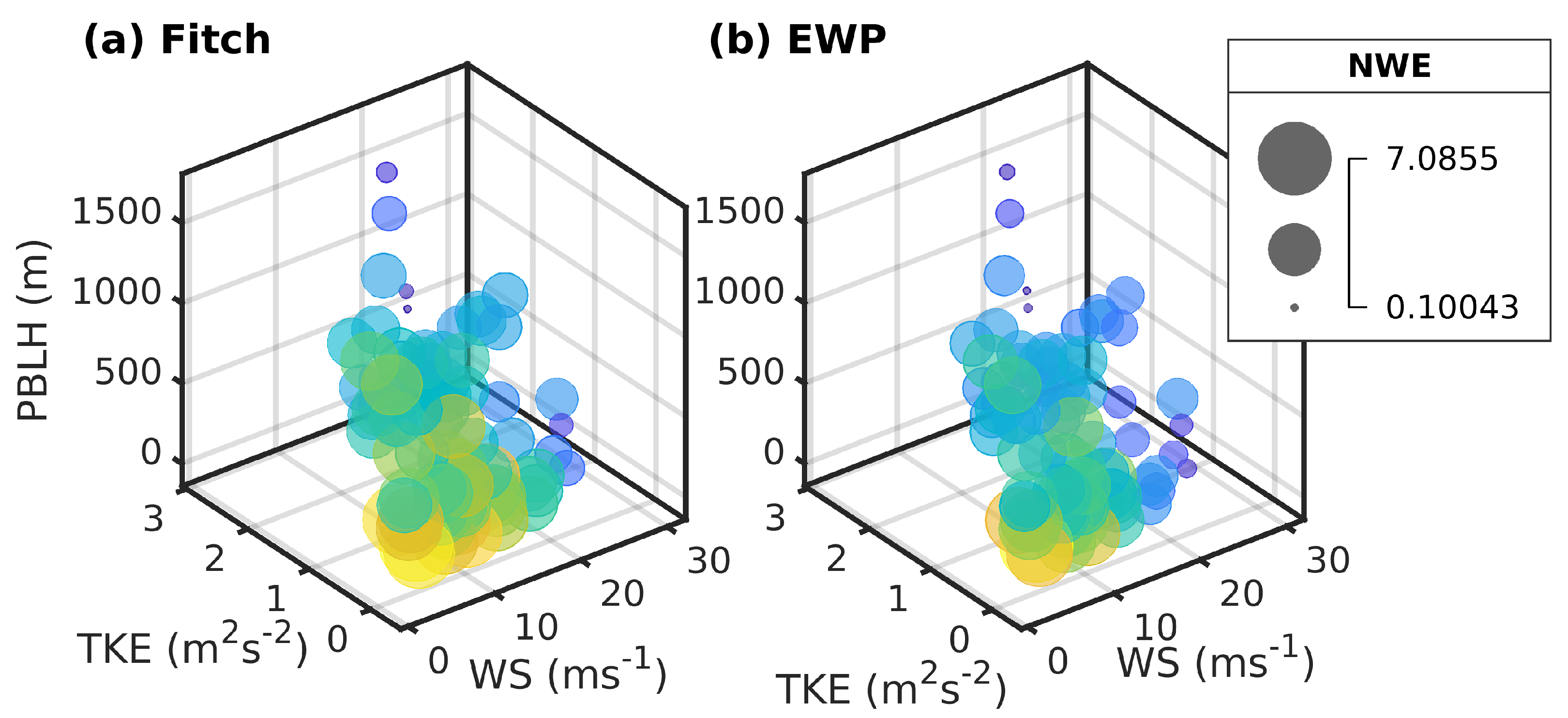
3.3. NWE Physical Dependencies: Building an Emulator
3.4. Deep Array Effect
4. Discussion: Caveats
- ○
- Code correction in v4.1.3: ‘When using the MYNN PBL scheme, with icloud_bl = 1 (which is default), restarts did not give bit-for-bit results when compared to a non-restart run. This has been a problem since the option was introduced in V3.8, but is now corrected.’
- ○
- Code correction in v4.1: ‘MYNN Updates: The biggest improvement is the reduction in the downward shortwave radiation bias through better cloud fraction and subgrid scale mixing ratios.’
- ○
- Default mixing length in MYNN in v3.8 was ‘RAP/HRRR (including BouLac in free atmosphere)’ (https://www2.mmm.ucar.edu/wrf/users/docs/user_guide_V3/user_guide_V3.8/users_guide_chap5.htm, accessed on 1 November 2023) but was changed by v4.2 to ‘experimental (includes cloud-specific mixing length and a scale-aware mixing length; following Ito et al. 2015, BLM); this option has been well-tested with the edmf options.’ (https://www2.mmm.ucar.edu/wrf/users/docs/user_guide_v4/v4.2/users_guide_chap5.html, accessed on 1 November 2023). In brief, Ito et al. [98] proposed a modification to the MYNN scheme wherein the mixing length scale is defined so that turbulence kinetic energy (TKE) dissipation is invariant with dx.
5. Conclusions
Author Contributions
Funding
Data Availability Statement
Acknowledgments
Conflicts of Interest
References
- Barthelmie, R.J.; Pryor, S.C. Climate Change Mitigation Potential of Wind Energy. Climate 2021, 9, 136. [Google Scholar] [CrossRef]
- Rigano, J.P.; Delle Fave, A. Offshore wind: Government control and the regulatory landscape. Environ. Claims J. 2017, 29, 80–85. [Google Scholar] [CrossRef]
- Global Wind Energy Council. Global Wind Report 2023; Global Wind Energy Council: Brussels, Belgium, 2023; p. 118. Available online: https://gwec.net/gwecs-global-offshore-wind-report-2023/ (accessed on 1 November 2023).
- Shields, M.; Stefek, J.; Oteri, F.; Kreider, M.; Gill, E.; Maniak, S.; Gould, R.; Malvik, C.; Tirone, S.; Hines, E. A Supply Chain Road Map for Offshore Wind Energy in the United States; National Renewable Energy Lab.(NREL): Golden, CO, USA, 2023. Available online: https://www.osti.gov/biblio/1922189 (accessed on 1 November 2023).
- Soares-Ramos, E.P.; de Oliveira-Assis, L.; Sarrias-Mena, R.; Fernández-Ramírez, L.M. Current status and future trends of offshore wind power in Europe. Energy 2020, 202, 117787. [Google Scholar] [CrossRef]
- Sovacool, B.K.; Enevoldsen, P.; Koch, C.; Barthelmie, R.J. Cost performance and risk in the construction of offshore and onshore wind farms. Wind Energy 2017, 20, 891–908. [Google Scholar] [CrossRef]
- Barthelmie, R.J.; Courtney, M.S.; Hojstrup, H.; Larsen, S.E. Meteorological aspects of offshore wind energy: Observations from the Vindeby wind farm. J. Wind Eng. Ind. Aerodyn. 1996, 62, 191–211. [Google Scholar] [CrossRef]
- Jansen, M.; Staffell, I.; Kitzing, L.; Quoilin, S.; Wiggelinkhuizen, E.; Bulder, B.; Riepin, I.; Müsgens, F. Offshore wind competitiveness in mature markets without subsidy. Nat. Energy 2020, 5, 614–622. [Google Scholar] [CrossRef]
- Díaz, H.; Soares, C.G. Review of the current status, technology and future trends of offshore wind farms. Ocean Eng. 2020, 209, 107381. [Google Scholar] [CrossRef]
- Ahsbahs, T.; Maclaurin, G.; Draxl, C.; Jackson, C.; Monaldo, F.; Badger, M. US East Coast synthetic aperture radar wind atlas for offshore wind energy. Wind Energy Sci. 2020, 5, 1191–1210. [Google Scholar] [CrossRef]
- Musial, W.; Heimiller, D.; Beiter, P.; Scott, G.; Draxl, C. 2016 Offshore Wind Energy Resource Assessment for the United States; Technical Report NREL/TP-5000-66599; National Renewable Energy Laboratory: Golden, CO, USA, 2016; p. 88. Available online: https://www.nrel.gov/docs/fy16osti/66599.pdf (accessed on 16 July 2020).
- Barthelmie, R.J.; Dantuono, K.; Renner, E.; Letson, F.; Pryor, S.C. Extreme wind and waves in U.S. east coast offshore wind energy lease areas. Energies 2021, 14, 1053. [Google Scholar] [CrossRef]
- DeCastro, M.; Salvador, S.; Gómez-Gesteira, M.; Costoya, X.; Carvalho, D.; Sanz-Larruga, F.; Gimeno, L. Europe, China and the United States: Three different approaches to the development of offshore wind energy. Renew. Sustain. Energy Rev. 2019, 109, 55–70. [Google Scholar] [CrossRef]
- Pryor, S.C.; Barthelmie, R.J.; Shepherd, T.J. Wind power production from very large offshore wind farms. Joule 2021, 5, 2663–2686. [Google Scholar] [CrossRef]
- Mills, A.D.; Millstein, D.; Jeong, S.; Lavin, L.; Wiser, R.; Bolinger, M. Estimating the value of offshore wind along the United States’ eastern coast. Environ. Res. Lett. 2018, 13, 09401310. [Google Scholar] [CrossRef]
- Musial, W.; Spitsen, P.; Duffy, P.; Beiter, P.; Marquis, M.; Hammond, R.; Shields, M. Offshore Wind Market Report: 2022 Edition; USDOE Office of Energy Efficiency and Renewable Energy (EERE), Wind Energy Technologies Office (EE-4W); U.S. Department of Energy Office of Scientific and Technical Information: Oak Ridge, TN, USA, 2022. [CrossRef]
- Pryor, S.C.; Barthelmie, R.J. Wind shadows impact planning of large offshore wind farms. Appl. Energy 2024, 359, 122755. [Google Scholar] [CrossRef]
- Lundquist, J.; DuVivier, K.; Kaffine, D.; Tomaszewski, J. Costs and consequences of wind turbine wake effects arising from uncoordinated wind energy development. Nat. Energy 2019, 4, 26–34. [Google Scholar] [CrossRef]
- Howland, M.F.; Quesada, J.B.; Martínez, J.J.P.; Larrañaga, F.P.; Yadav, N.; Chawla, J.S.; Sivaram, V.; Dabiri, J.O. Collective wind farm operation based on a predictive model increases utility-scale energy production. Nat. Energy 2022, 7, 818–827. [Google Scholar] [CrossRef]
- Finserås, E.; Anchustegui, I.H.; Cheynet, E.; Gebhardt, C.G.; Reuder, J. Gone with the wind? Wind farm-induced wakes and regulatory gaps. Mar. Policy 2024, 159, 105897. [Google Scholar] [CrossRef]
- Jansen, M.; Beiter, P.; Riepin, I.; Müsgens, F.; Guajardo-Fajardo, V.J.; Staffell, I.; Bulder, B.; Kitzing, L. Policy choices and outcomes for offshore wind auctions globally. Energy Policy 2022, 167, 113000. [Google Scholar] [CrossRef]
- Johnston, B.; Foley, A.; Doran, J.; Littler, T. Levelised cost of energy, A challenge for offshore wind. Renew. Energy 2020, 160, 876–885. [Google Scholar] [CrossRef]
- Caputo, A.C.; Federici, A.; Pelagagge, P.M.; Salini, P. Offshore wind power system economic evaluation framework under aleatory and epistemic uncertainty. Appl. Energy 2023, 350, 121585. [Google Scholar] [CrossRef]
- Ioannou, A.; Angus, A.; Brennan, F. Stochastic financial appraisal of offshore wind farms. Renew. Energy 2020, 145, 1176–1191. [Google Scholar] [CrossRef]
- Đukan, M.; Kitzing, L. The impact of auctions on financing conditions and cost of capital for wind energy projects. Energy Policy 2021, 152, 112197. [Google Scholar] [CrossRef]
- Wind Europe. Offshore Wind in Europe Key Trends and Statistics; Wind Europe: Brussels, Belgium, 2020; p. 40. Available online: https://windeurope.org/wp-content/uploads/files/about-wind/statistics/WindEurope-Annual-Offshore-Statistics-2019.pdf (accessed on 27 February 2020).
- Bosch, J.; Staffell, I.; Hawkes, A.D. Global levelised cost of electricity from offshore wind. Energy 2019, 189, 116357. [Google Scholar] [CrossRef]
- Deutsche Wind Guard GmbH. Capacity Densities of European Offshore Wind Farms; Deutsche Wind Guard GmbH: Hamburg, Germany, 2018; p. 76. Available online: https://www.msp-platform.eu/practices/capacity-densities-european-offshore-wind-farms (accessed on 1 November 2023).
- Barthelmie, R.J.; Hansen, K.S.; Pryor, S.C. Meteorological controls on wind turbine wakes. Proc. IEEE 2013, 101, 1010–1019. [Google Scholar] [CrossRef]
- Barthelmie, R.J.; Jensen, L.E. Evaluation of wind farm efficiency and wind turbine wakes at the Nysted offshore wind farm. Wind Energy 2010, 13, 573–586. [Google Scholar] [CrossRef]
- Thomsen, K.; Sørensen, P. Fatigue loads for wind turbines operating in wakes. J. Wind Eng. Ind. Aerodyn. 1999, 80, 121–136. [Google Scholar] [CrossRef]
- Barthelmie, R.J.; Pryor, S.C.; Frandsen, S.T.; Hansen, K.; Schepers, J.G.; Rados, K.; Schlez, W.; Neubert, A.; Jensen, L.E.; Neckelmann, S. Quantifying the impact of wind turbine wakes on power output at offshore wind farms. J. Atmos. Ocean. Technol. 2010, 27, 1302–1317. [Google Scholar] [CrossRef]
- Hasager, C.B.; Vincent, P.; Badger, J.; Badger, M.; Di Bella, A.; Peña, A.; Husson, R.; Volker, P.J. Using satellite SAR to characterize the wind flow around offshore wind farms. Energies 2015, 8, 5413–5439. [Google Scholar] [CrossRef]
- Pryor, S.C.; Shepherd, T.J.; Volker, P.; Hahmann, A.N.; Barthelmie, R.J. ‘Wind theft’ from onshore wind turbine arrays: Sensitivity to wind farm parameterization and resolution. J. Appl. Meteorol. Climatol. 2020, 59, 153–174. [Google Scholar] [CrossRef]
- Wu, Y.-T.; Porté-Agel, F. Atmospheric turbulence effects on wind-turbine wakes: An LES study. Energies 2012, 5, 5340–5362. [Google Scholar] [CrossRef]
- Lee, J.C.; Lundquist, J.K. Observing and simulating wind-turbine wakes during the evening transition. Bound.-Layer Meteorol. 2017, 164, 449–474. [Google Scholar] [CrossRef]
- Enevoldsen, P.; Valentine, S.V. Do onshore and offshore wind farm development patterns differ? Energy Sustain. Dev. 2016, 35, 41–51. [Google Scholar] [CrossRef]
- Enevoldsen, P.; Xydis, G. Examining the trends of 35 years growth of key wind turbine components. Energy Sustain. Dev. 2019, 50, 18–26. [Google Scholar] [CrossRef]
- Sickler, M.; Ummels, B.; Zaaijer, M.; Schmehl, R.; Dykes, K. Offshore wind farm optimisation: A comparison of performance between regular and irregular wind turbine layouts. Wind Energy Sci. 2023, 8, 1225–1233. [Google Scholar] [CrossRef]
- Bensason, D.; Simley, E.; Roberts, O.; Fleming, P.; Debnath, M.; King, J.; Bay, C.; Mudafort, R. Evaluation of the potential for wake steering for US land-based wind power plants. J. Renew. Sustain. Energy 2021, 13, 033303. [Google Scholar] [CrossRef]
- Staid, A.; VerHulst, C.; Guikema, S.D. A comparison of methods for assessing power output in non-uniform onshore wind farms. Wind Energy 2018, 21, 42–52. [Google Scholar] [CrossRef]
- Doekemeijer, B.M.; Simley, E.; Fleming, P. Comparison of the Gaussian wind farm model with historical data of three offshore wind farms. Energies 2022, 15, 1964. [Google Scholar] [CrossRef]
- Ali, K.; Schultz, D.M.; Revell, A.; Stallard, T.; Ouro, P. Assessment of five wind-farm parameterizations in the Weather Research and Forecasting model: A case study of wind farms in the North Sea. Mon. Weather Rev. 2023, 151, 2333–2359. [Google Scholar] [CrossRef]
- Xie, B.; Fung, J.C.; Chan, A.; Lau, A. Evaluation of nonlocal and local planetary boundary layer schemes in the WRF model. J. Geophys. Res. Atmos. 2012, 117, D12103. [Google Scholar] [CrossRef]
- Peña, A.; Hahmann, A.N. Atmospheric stability and turbulence fluxes at Horns Rev—An intercomparison of sonic, bulk and WRF model data. Wind Energy 2012, 15, 717–731. [Google Scholar] [CrossRef]
- Stevens, R.J.; Meneveau, C. Flow structure and turbulence in wind farms. Annu. Rev. Fluid Mech. 2017, 49, 311–339. [Google Scholar] [CrossRef]
- Miller, L.M.; Brunsell, N.A.; Mechem, D.B.; Gans, F.; Monaghan, A.J.; Vautard, R.; Keith, D.W.; Kleidon, A. Two methods for estimating limits to large-scale wind power generation. Proc. Natl. Acad. Sci. USA 2015, 112, 11169–11174. [Google Scholar] [CrossRef] [PubMed]
- Volker, P.J.H.; Hahmann, A.N.; Badger, J.; Jørgensen, H.E. Prospects for generating electricity by large onshore and offshore wind farms. Environ. Res. Lett. 2017, 12, 034022. [Google Scholar] [CrossRef]
- Christiansen, M.B.; Hasager, C. Wake effects of large offshore wind farms identified from satellite SAR. Remote Sens. Environ. 2005, 98, 251–268. [Google Scholar] [CrossRef]
- Eriksson, O.; Mikkelsen, R.; Hansen, K.S.; Nilsson, K.; Ivanell, S. Analysis of long distance wakes of Horns Rev I using actuator disc approach. J. Phys. Conf. Ser. 2014, 555, 012032. [Google Scholar] [CrossRef]
- Ahsbahs, T.; Nygaard, N.G.; Newcombe, A.; Badger, M. Wind farm wakes from SAR and doppler radar. Remote Sens. 2020, 12, 462. [Google Scholar] [CrossRef]
- Nygaard, N.G.; Newcombe, A.C. Wake behind an offshore wind farm observed with dual-Doppler radars. J. Phys. Conf. Ser. 2018, 1037, 072008. [Google Scholar] [CrossRef]
- Cañadillas, B.; Beckenbauer, M.; Trujillo, J.J.; Dörenkämper, M.; Foreman, R.; Neumann, T.; Lampert, A. Offshore wind farm cluster wakes as observed by long-range-scanning wind lidar measurements and mesoscale modeling. Wind Energy Sci. 2022, 7, 1241–1262. [Google Scholar] [CrossRef]
- Platis, A.; Siedersleben, S.K.; Bange, J.; Lampert, A.; Bärfuss, K.; Hankers, R.; Cañadillas, B.; Foreman, R.; Schulz-Stellenfleth, J.; Djath, B.; et al. First in situ evidence of wakes in the far field behind offshore wind farms. Sci. Rep. 2018, 8, 2163. [Google Scholar] [CrossRef]
- Cañadillas, B.; Foreman, R.; Barth, V.; Siedersleben, S.; Lampert, A.; Platis, A.; Djath, B.; Schulz-Stellenfleth, J.; Bange, J.; Emeis, S. Offshore wind farm wake recovery: Airborne measurements and its representation in engineering models. Wind Energy 2020, 23, 1249–1265. [Google Scholar] [CrossRef]
- Fischereit, J.; Brown, R.; Larsén, X.G.; Badger, J.; Hawkes, G. Review of Mesoscale Wind-Farm Parametrizations and Their Applications. Bound.-Layer Meteorol. 2022, 182, 175–224. [Google Scholar] [CrossRef]
- Cuevas-Figueroa, G.; Stansby, P.K.; Stallard, T. Accuracy of WRF for prediction of operational wind farm data and assessment of influence of upwind farms on power production. Energy 2022, 254, 124362. [Google Scholar] [CrossRef]
- Hahmann, A.N.; Sile, T.; Witha, B.; Davis, N.N.; Dörenkämper, M.; Ezber, Y.; García-Bustamante, E.; González Rouco, J.F.; Navarro, J.; Olsen, B.T.; et al. The Making of the New European Wind Atlas, Part 1: Model Sensitivity. Geosci. Model Dev. 2020, 13, 5053–5078. [Google Scholar] [CrossRef]
- Pryor, S.C.; Coburn, J.J.; Barthelmie, R.J.; Shepherd, T.J. Projecting Future Energy Production from Operating Wind Farms in North America: Part 1: Dynamical Downscaling. J. Appl. Meteorol. Climatol. 2022, 62, 63–80. [Google Scholar] [CrossRef]
- Losada Carreño, I.; Craig, M.T.; Rossol, M.; Ashfaq, M.; Batibeniz, F.; Haupt, S.E.; Draxl, C.; Hodge, B.-M.; Brancucci, C. Potential impacts of climate change on wind and solar electricity generation in Texas. Clim. Chang. 2020, 163, 745–766. [Google Scholar] [CrossRef]
- Xu, W.; Liu, P.; Cheng, L.; Zhou, Y.; Xia, Q.; Gong, Y.; Liu, Y. Multi-step wind speed prediction by combining a WRF simulation and an error correction strategy. Renew. Energy 2021, 163, 772–782. [Google Scholar] [CrossRef]
- Xing, Y.; Lien, F.-S.; Melek, W.; Yee, E. A Multi-Hour Ahead Wind Power Forecasting System Based on a WRF-TOPSIS-ANFIS Model. Energies 2022, 15, 5472. [Google Scholar] [CrossRef]
- Haupt, S.E.; McCandless, T.C.; Dettling, S.; Alessandrini, S.; Lee, J.A.; Linden, S.; Petzke, W.; Brummet, T.; Nguyen, N.; Kosović, B. Combining artificial intelligence with physics-based methods for probabilistic renewable energy forecasting. Energies 2020, 13, 1979. [Google Scholar] [CrossRef]
- Fitch, A.C.; Olson, J.B.; Lundquist, J.K.; Dudhia, J.; Gupta, A.K.; Michalakes, J.; Barstad, I. Local and Mesoscale Impacts of Wind Farms as Parameterized in a Mesoscale NWP Model. Mon. Weather Rev. 2012, 140, 3017–3038. [Google Scholar] [CrossRef]
- Volker, P.J.H.; Badger, J.; Hahmann, A.N.; Ott, S. The Explicit Wake Parametrisation V1.0: A wind farm parametrisation in the mesoscale model WRF. Geosci. Model Dev. 2015, 8, 3481–3522. [Google Scholar] [CrossRef]
- Archer, C.L.; Wu, S.; Ma, Y.; Jiménez, P.A. Two corrections for turbulent kinetic energy generated by wind farms in the WRF model. Mon. Weather Rev. 2020, 148, 4823–4835. [Google Scholar] [CrossRef]
- Shepherd, T.J.; Barthelmie, R.J.; Pryor, S.C. Sensitivity of wind turbine array downstream effects to the parameterization used in WRF. J. Appl. Meteorol. Climatol. 2020, 59, 333–361. [Google Scholar] [CrossRef]
- Pryor, S.C.; Shepherd, T.; Volker, P.; Hahmann, A.; Barthelmie, R.J. Diagnosing systematic differences in predicted wind turbine array-array interactions. J. Phys. Conf. Series. Sci. Mak. Torque Wind. 2020, 1618, 062023. [Google Scholar] [CrossRef]
- Siedersleben, S.K.; Platis, A.; Lundquist, J.K.; Djath, B.; Lampert, A.; Bärfuss, K.; Canadillas, B.; Schultz-Stellenfleth, J.; Bange, J.; Neumann, T.; et al. Observed and simulated turbulent kinetic energy (WRF 3.8.1) overlarge offshore wind farms. Geosci. Model Dev. 2020, 13, 249–268. [Google Scholar] [CrossRef]
- Larsén, X.G.; Fischereit, J. A case study of wind farm effects using two wake parameterizations in the Weather Research and Forecasting (WRF) model (V3. 7.1) in the presence of low-level jets. Geosci. Model Dev. 2021, 14, 3141–3158. [Google Scholar] [CrossRef]
- Garcia-Santiago, O.M.; Badger, J.; Hahmann, A.N.; da Costa, G.L. Evaluation of two mesoscale wind farm parametrisations with offshore tall masts. J. Phys. Conf. Ser. 2022, 2265, 022038. [Google Scholar] [CrossRef]
- Fischereit, J.; Schaldemose Hansen, K.; Larsén, X.G.; van der Laan, M.P.; Réthoré, P.-E.; Murcia Leon, J.P. Comparing and validating intra-farm and farm-to-farm wakes across different mesoscale and high-resolution wake models. Wind Energy Sci. 2022, 7, 1069–1091. [Google Scholar] [CrossRef]
- Rybchuk, A.; Juliano, T.W.; Lundquist, J.K.; Rosencrans, D.; Bodini, N.; Optis, M. The sensitivity of the fitch wind farm parameterization to a three-dimensional planetary boundary layer scheme. Wind Energy Sci. 2022, 7, 2085–2098. [Google Scholar] [CrossRef]
- Bureau of Ocean Energy Management. Outer Continental Shelf: Renewable Energy Leases Map Book; U.S. Department of the Interior: Bureau of Ocean Energy Management: Sterling, VA, USA, 2022; p. 33. Available online: https://www.boem.gov/renewable-energy/mapping-and-data/renewable-energy-gis-data (accessed on 1 November 2023).
- Schneemann, J.; Rott, A.; Dörenkämper, M.; Steinfeld, G.; Kühn, M. Cluster wakes impact on a far-distant offshore wind farm’s power. Wind Energy Sci. 2020, 5, 29–49. [Google Scholar] [CrossRef]
- Mlawer, E.J.; Taubman, S.J.; Brown, P.D.; Iacono, M.J.; Clough, S.A. Radiative transfer for inhomogeneous atmospheres: RRTM, a validated correlated-k model for the longwave. J. Geophys. Res. Atmos. 1997, 102, 16663–16682. [Google Scholar] [CrossRef]
- Dudhia, J. Numerical study of convection observed during the winter monsoon experiment using a mesoscale two-dimensional model. J. Atmos. Sci. 1989, 46, 3077–3107. [Google Scholar] [CrossRef]
- Ferrier, B.S.; Jin, Y.; Lin, Y.; Black, T.; Rogers, E.; DiMego, G. Implementation of a new grid-scale cloud and precipitation scheme in the NCEP Eta model. In Proceedings of the 15th Conference on Numerical Weather Prediction, San Antonio, TX, USA, 12–16 August 2002; pp. 280–283. [Google Scholar]
- Kain, J.S. The Kain–Fritsch convective parameterization: An update. J. Appl. Meteorol. 2004, 43, 170–181. [Google Scholar] [CrossRef]
- Beljaars, A. The parametrization of surface fluxes in large-scale models under free convection. Q. J. R. Meteorol. Soc. 1995, 121, 255–270. [Google Scholar]
- Tewari, M.; Chen, F.; Wang, W.; Dudhia, J.; LeMone, M.; Mitchell, K.; Ek, M.; Gayno, G.; Wegiel, J.; Cuenca, R. Implementation and verification of the unified NOAH land surface model in the WRF model. In Proceedings of the 20th Conference on Weather Analysis and Forecasting/16th Conference on Numerical Weather Prediction, Seattle, WA, USA, 12–16 January 2004; Volume 1115. 6pAvailable online: https://ams.confex.com/ams/84Annual/techprogram/paper_69061.htm (accessed on 1 November 2023).
- Nakanishi, M.; Niino, H. An improved Mellor–Yamada level-3 model: Its numerical stability and application to a regional prediction of advection fog. Bound.-Layer Meteorol. 2006, 119, 397–407. [Google Scholar] [CrossRef]
- Foody, R.; Coburn, J.; Aird, J.A.; Barthelmie, R.J.; Pryor, S.C. Onshore and Offshore Wind Resources and Operating Conditions in the Eastern US. Wind Energy Sci. 2024, 9, 263–280. [Google Scholar] [CrossRef]
- Agora Engiewende; Agora Verkehrswende; Technical University of Denmark; Max-Planck-Institute for Biogeochemistry. Making the Most of Offshore Wind: Re-Evaluating the Potential of Offshore Wind in the German North Sea; 36-2020-EN; Agra Energiewende: Berlin, Germany, 2020; p. 80. Available online: https://www.agora-energiewende.de/en/publications/making-the-most-of-offshore-wind (accessed on 1 November 2023).
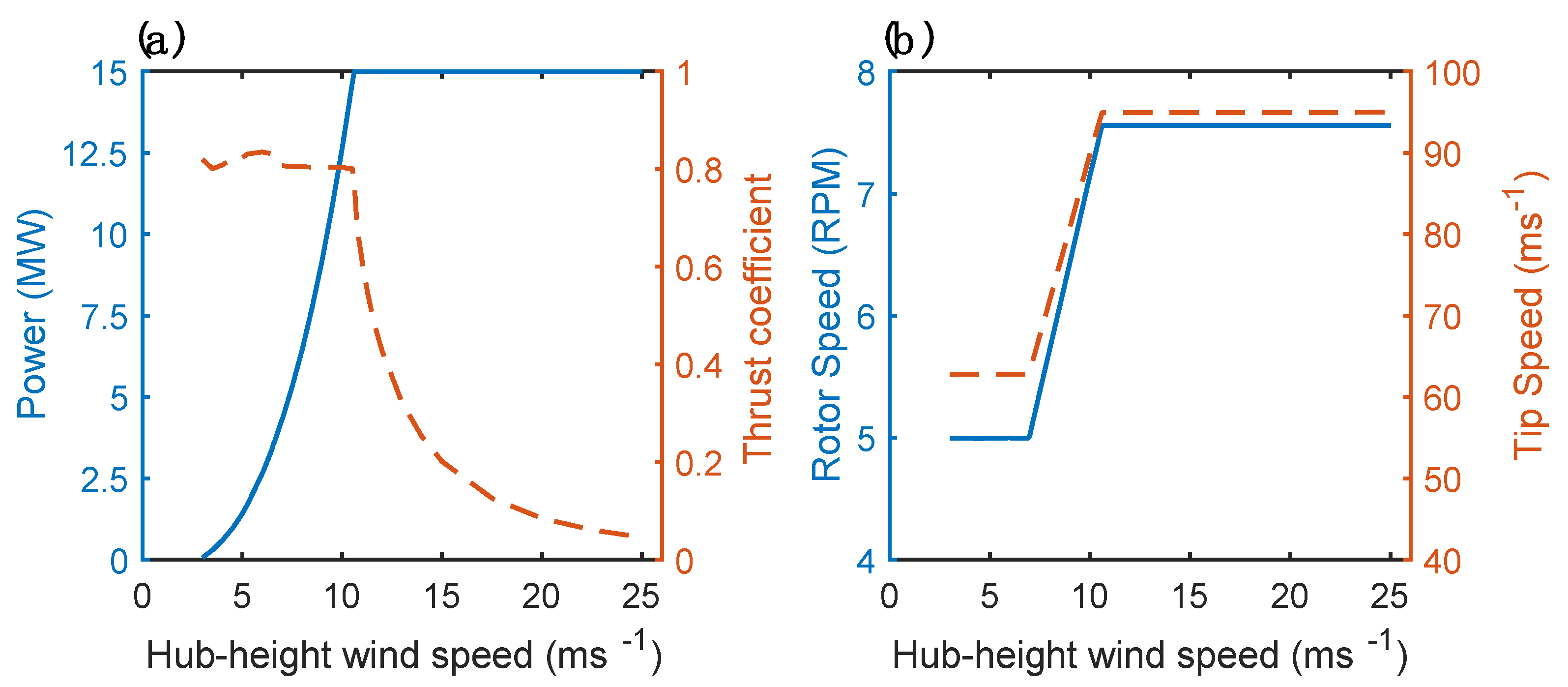
- Gaertner, E.; Rinker, J.; Sethuraman, L.; Zahle, F.; Anderson, B.; Barter, G.E.; Abbas, N.J.; Meng, F.; Bortolotti, P.; Skrzypinski, W. IEA Wind TCP Task 37: Definition of the IEA 15-Megawatt Offshore Reference Wind Turbine; National Renewable Energy Lab.(NREL): Golden, CO, USA, 2020; p. 44. Available online: https://www.osti.gov/biblio/1603478 (accessed on 1 November 2023).
- Hersbach, H.; Bell, B.; Berrisford, P.; Hirahara, S.; Horányi, A.; Muñoz-Sabater, J.; Nicolas, J.; Peubey, C.; Radu, R.; Schepers, D.; et al. The ERA5 global reanalysis. Q. J. R. Meteorol. Soc. 2020, 146, 1999–2049. [Google Scholar] [CrossRef]
- Wilks, D.S. Statistical Methods in the Atmospheric Sciences; Academic Press: Oxford, UK, 2011; Volume 100, ISBN 9780123850225. [Google Scholar]
- Debnath, M.; Doubrawa, P.; Optis, M.; Hawbecker, P.; Bodini, N. Extreme wind shear events in US offshore wind energy areas and the role of induced stratification. Wind Energy Sci. 2021, 6, 1043–1059. [Google Scholar] [CrossRef]
- National Renewable Energy Laboratory. 2023 National Offshore Wind Data Set (NOW-23); National Renewable Energy Laboratory: Golden, CO, USA, 2020. [CrossRef]
- Wu, Y.-T.; Porté-Agel, F. Simulation of Turbulent Flow Inside and Above Wind Farms: Model Validation and Layout Effects. Bound.-Layer Meteorol. 2013, 146, 181–205. [Google Scholar] [CrossRef]
- Ruiz-Arias, J.A.; Dudhia, J.; Santos-Alamillos, F.J.; Pozo-Vázquez, D. Surface clear-sky shortwave radiative closure intercomparisons in the Weather Research and Forecasting model. J. Geophys. Res. Atmos. 2013, 118, 9901–9913. [Google Scholar] [CrossRef]
- Mooney, P.; Mulligan, F.; Fealy, R. Evaluation of the sensitivity of the weather research and forecasting model to parameterization schemes for regional climates of Europe over the period 1990–1995. J. Clim. 2013, 26, 1002–1017. [Google Scholar] [CrossRef]
- Ma, Y.; Archer, C.L.; Vasel-Be-Hagh, A. Comparison of individual versus ensemble wind farm parameterizations inclusive of sub-grid wakes for the WRF model. Wind Energy 2022, 25, 1573–1595. [Google Scholar] [CrossRef]
- Eriksson, O.; Lindvall, J.; Breton, S.-P.; Ivanell, S. Wake downstream of the Lillgrund wind farm-A Comparison between LES using the actuator disc method and a wind farm parametrization in WRF. J. Phys. Conf. Ser. 2015, 625, 012028. [Google Scholar] [CrossRef]
- Sood, I.; Simon, E.; Vitsas, A.; Blockmans, B.; Larsen, G.C.; Meyers, J. Comparison of large eddy simulations against measurements from the Lillgrund offshore wind farm. Wind Energy Sci. 2022, 7, 2469–2489. [Google Scholar] [CrossRef]
- Maas, O.; Raasch, S. Wake properties and power output of very large wind farms for different meteorological conditions and turbine spacings: A large-eddy simulation case study for the German Bight. Wind Energy Sci. 2022, 7, 715–739. [Google Scholar] [CrossRef]
- Hsu, S.A.; Meindl, E.A.; Gilhousen, D.B. Determining the power-law wind-profile exponent under near-neutral stability conditions at sea. J. Appl. Meteorol. 1994, 33, 757–765. [Google Scholar] [CrossRef]
- Ito, J.; Niino, H.; Nakanishi, M.; Moeng, C.-H. An extension of the Mellor–Yamada model to the terra incognita zone for dry convective mixed layers in the free convection regime. Bound.-Layer Meteorol. 2015, 157, 23–43. [Google Scholar] [CrossRef]
- Yang, B.; Berg, L.K.; Qian, Y.; Wang, C.; Hou, Z.; Liu, Y.; Shin, H.H.; Hong, S.; Pekour, M. Parametric and structural sensitivities of turbine-height wind speeds in the boundary layer parameterizations in the weather research and forecasting model. J. Geophys. Res. Atmos. 2019, 124, 5951–5969. [Google Scholar] [CrossRef]
- Cazzaro, D.; Trivella, A.; Corman, F.; Pisinger, D. Multi-scale optimization of the design of offshore wind farms. Appl. Energy 2022, 314, 118830. [Google Scholar] [CrossRef]


| Layout | CNTRL | CORRI | 6MWSQ | NYBIG |
|---|---|---|---|---|
| ICD (MWkm−2) | 4.3 | 3.5 | 6.0 | 4.3 |
| Total areal coverage of wind turbines (km2) | 6566 | 6566 | 6566 | 8536 |
| Total number of 15 MW wind turbines | 1922 | 1604 | 2598 | 2495 |
| Installed capacity (MW) by LA cluster | ||||
| LA1–7 | 16,095 | 13,500 | 22,275 | 16,095 |
| LA8 (plus NYBig for NYBIG) | 1335 | 1110 | 1875 | 9930 |
| LA9–13 | 9360 | 7815 | 12,195 | 9360 |
| LA14 and 15 | 2040 | 1635 | 2625 | 2040 |
| Layout | CNTRL | CORRI | 6MWSQ | NYBIG | ||||||
|---|---|---|---|---|---|---|---|---|---|---|
| ICD (MWkm−2) | 4.3 | 3.5 | 6.0 | 4.3 | ||||||
| Areal Coverage of Wind Turbines (km2) | 6566 | 6566 | 6566 | 8536 | ||||||
| Flow Scenario (WDWS) | Percent Frequency | Five-Day Simulation Period (YYYY-MM-DD) | Fitch | EWP | Fitch | EWP | Fitch | EWP | Fitch | EWP |
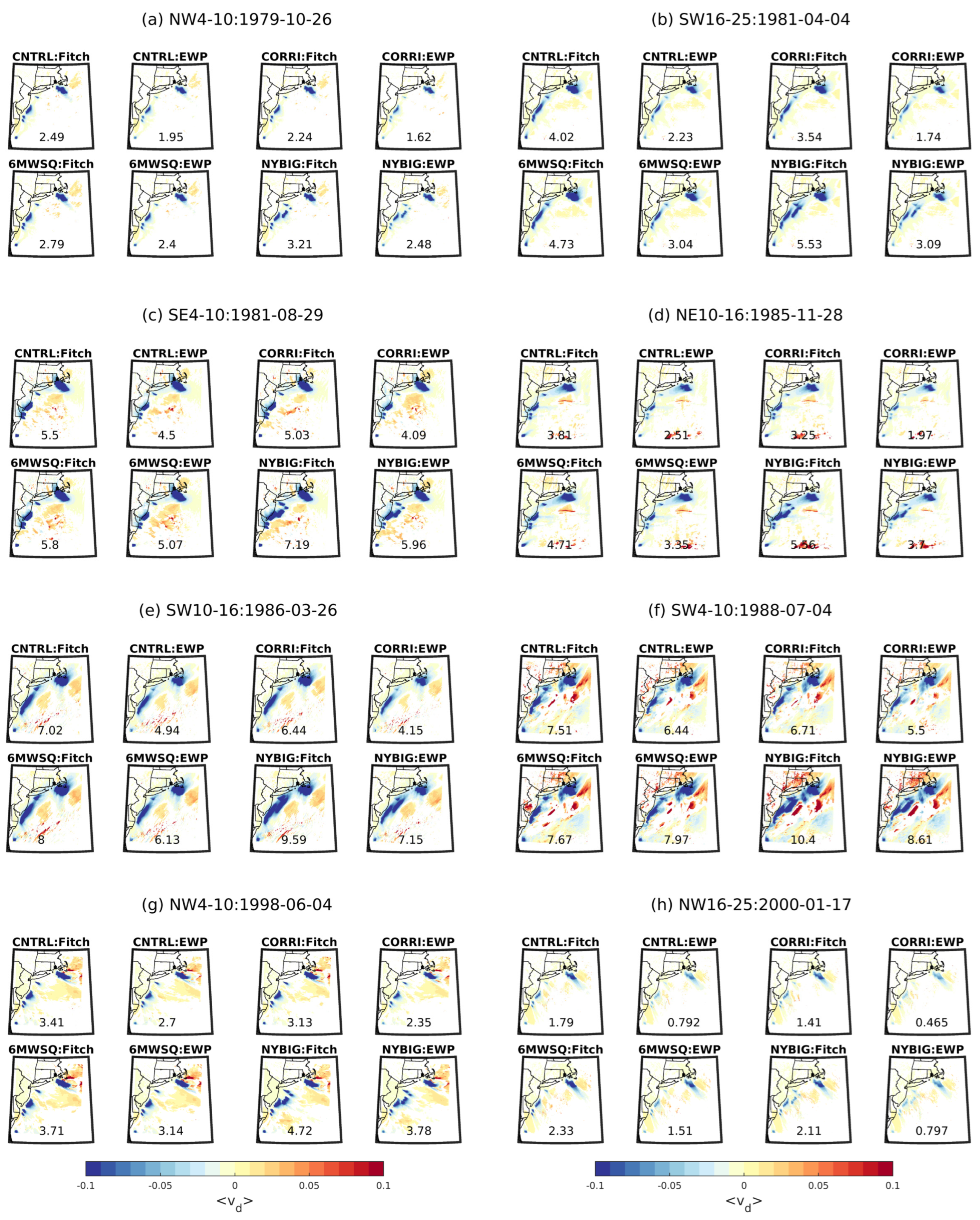
| NW4–10 | 7.85 | 1979-10-26 to 1979-10-30 | 2.49 | 1.95 | 2.24 | 1.62 | 2.79 | 2.40 | 3.21 | 2.48 |
| SW16–25 | 1.6 | 1981-04-04 to 1981-04-08 | 4.02 | 2.23 | 3.54 | 1.74 | 4.73 | 3.04 | 5.53 | 3.09 |
| SE4–10 | 7.5 | 1981-08-29 to 1981-09-02 | 5.50 | 4.50 | 5.03 | 4.09 | 5.80 | 5.07 | 7.19 | 5.96 |
| NE10–16 | 4.6 | 1985-11-28 to 1985-12-02 | 3.81 | 2.51 | 3.25 | 1.97 | 4.71 | 3.35 | 5.56 | 3.70 |
| SW10–16 | 9.1 | 1986-03-26 to 1986-03-30 | 7.02 | 4.94 | 6.44 | 4.15 | 8.00 | 6.13 | 9.59 | 7.15 |
| SW4–10 | 12.5 | 1988-07-04 to 1988-07-08 | 7.51 | 6.44 | 6.71 | 5.50 | 7.67 | 7.97 | 10.36 | 8.61 |
| NW4–10 | 7.85 | 1998-06-04 to 1998-06-08 | 3.41 | 2.70 | 3.13 | 2.35 | 3.71 | 3.14 | 4.72 | 3.78 |
| NW16–25 | 1.4 | 2000-01-17 to 2000-01-21 | 1.79 | 0.79 | 1.41 | 0.46 | 2.33 | 1.51 | 2.11 | 0.80 |
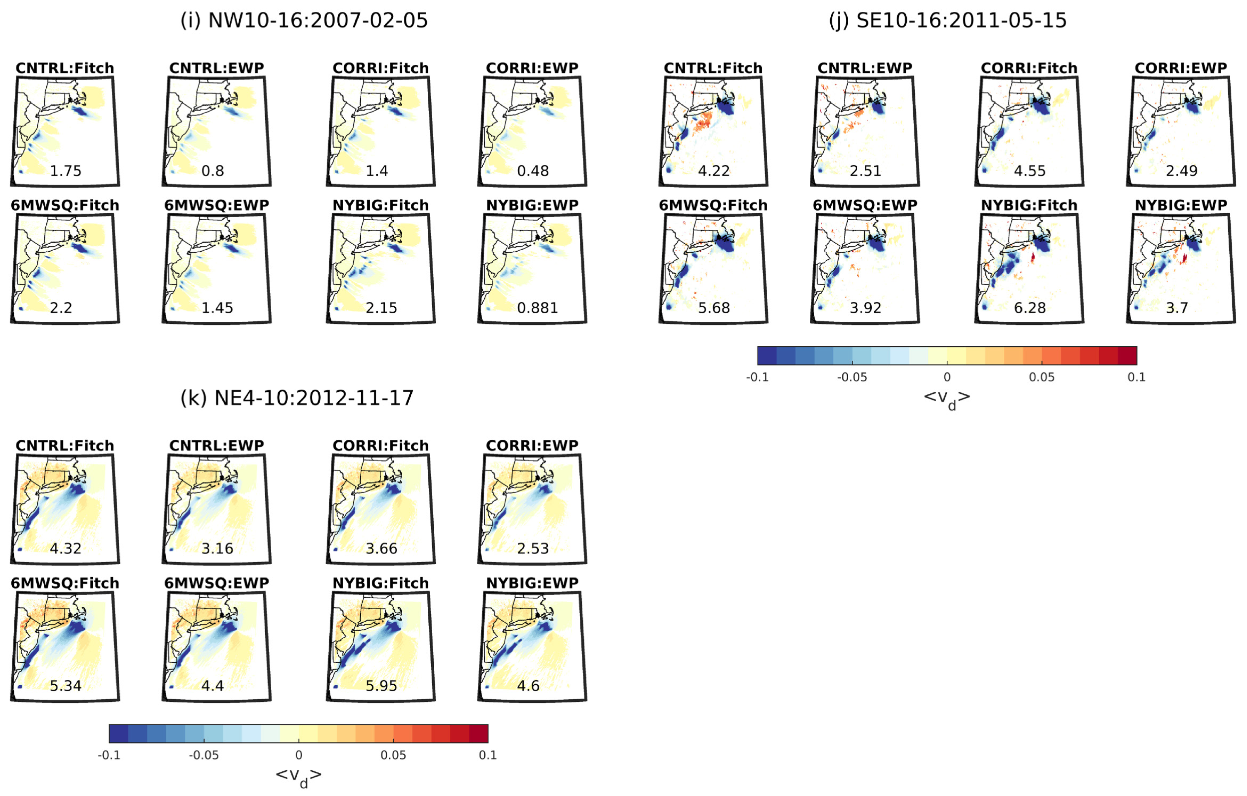
| NW10–16 | 11 | 2007-02-05 to 2007-02-09 | 1.75 | 0.80 | 1.40 | 0.48 | 2.20 | 1.45 | 2.15 | 0.88 |
| SE10–16 | 2.3 | 2011-05-15 to 2011-05-19 | 4.22 | 2.51 | 4.55 | 2.49 | 5.68 | 3.92 | 6.28 | 3.70 |
| NE4–10 | 9.6 | 2012-11-17 to 2012-11-21 | 4.32 | 3.16 | 3.66 | 2.53 | 5.34 | 4.40 | 5.95 | 4.60 |
| Metric | Description | Calculation Method (and Equation #) |
|---|---|---|
| Power production (PP in MWh) | Annual electrical power production in MWh from wind turbines | (2) = sum of power (in W) in each grid cell with wind turbine(s) (n = 1 to m) output every ten minutes (i = 1 to 720) from the WRF-WFP and computed via the power curve (division by 6 is to convert to Wh). = frequency weight of each of the 11 cases (j = 1 to 11) and then the resulting power is summed. The last two terms are first to scale to the number of hours in a full year from the number of simulated hours, and then to convert to MWh from Wh |
| Capacity factor (CF in %) | Simulated power production (PP) divided by that possible if all wind turbines operated at their rated capacity in each hour of the year | (3) |
| Wake-induced power losses (WL in MWh) | Amount of power production suppression due to wake reduction of inflow wind speed | (4) Potential power from each wind turbine computed from freestream windspeed (output from domain d03, WSfreestream) minus calculated power production from WFP |
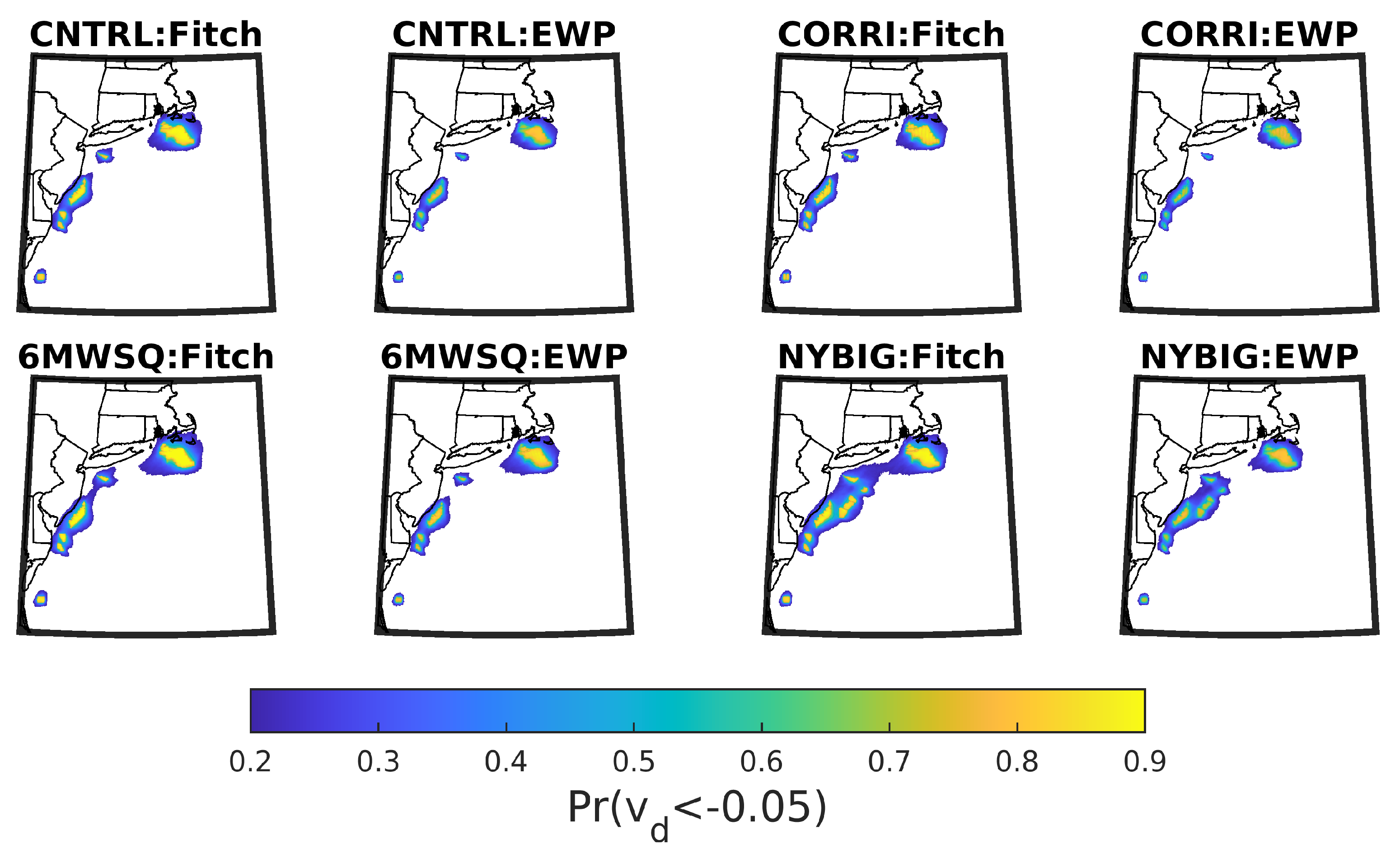
| Wake-induced velocity deficit | Normalized difference between wind speed computed at a given location and time from d04 or d05, relative to the freestream (domain d03) | (5) WSWT(x,y,i) indicates the wind speed when the WFP is operational (i.e., output from domain d04 (Fitch) or d05 (EWP)), WSNoWT denotes WS from the same location (x,y) and time stamp (i) but for domain 03 |
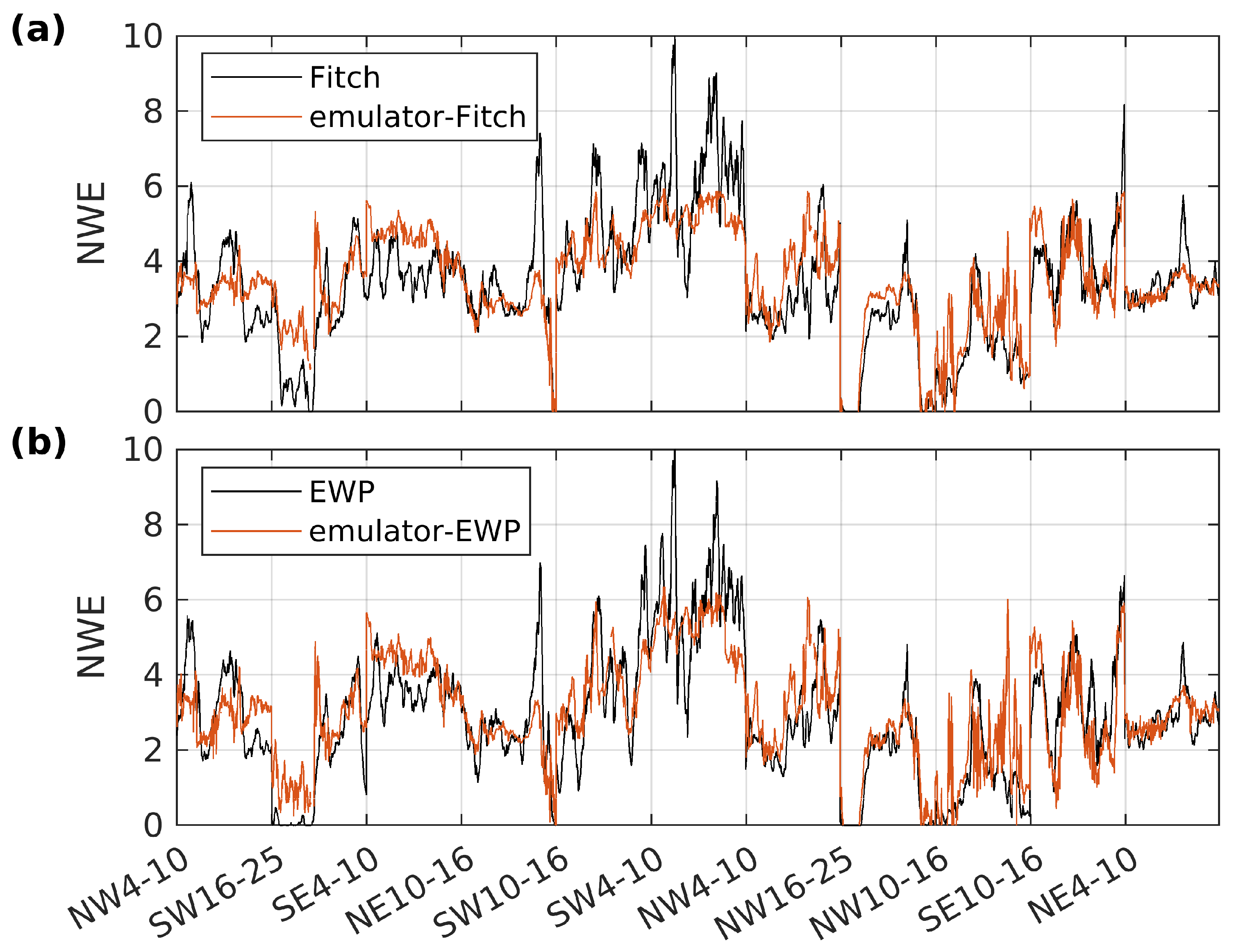
| Normalized wake extent (NWE) | Area with a velocity deficit of a given magnitude (X) divided by the footprint of the wind farm/lease area cluster | (6) |
| WFP: Lease Areas | System-Wide, i.e., All LAs | LA1–7 | LA8 * | LA9–13 | LA14 and 15 |
|---|---|---|---|---|---|
| EWP: CNTRL | 53.2 | 53.1 | 61.2 | 53.3 | 47.6 |
| EWP: CORRI | 54.9 | 54.9 | 62.4 | 55.0 | 48.5 |
| EWP: 6MWSQ | 49.7 | 49.2 | 58.3 | 50.0 | 45.2 |
| EWP: NYBIG | 52.6 | 53.0 | 52.7 | 51.5 | 47.6 |
| Fitch: CNTRL | 42.9 | 42.6 | 51.6 | 42.7 | 39.5 |
| Fitch: CORRI | 44.8 | 44.7 | 53.0 | 44.7 | 40.6 |
| Fitch: 6MWSQ | 38.7 | 38.1 | 47.7 | 38.9 | 36.4 |
| Fitch: NYBIG | 42.4 | 42.6 | 42.6 | 41.2 | 39.6 |
| Normalized difference: (Fitch-EWP)/Fitch | |||||
| CNTRL | −0.24 | −0.25 | −0.19 | −0.25 | −0.20 |
| CORRI | −0.23 | −0.23 | −0.18 | −0.23 | −0.20 |
| 6MWSQ | −0.28 | −0.29 | −0.22 | −0.29 | −0.24 |
| NYBIG | −0.24 | −0.24 | −0.24 | −0.25 | −0.20 |
| Layout | Fitch | EWP |
|---|---|---|
| CNTRL | 12.6 | 9.84 |
| CORRI | 11.5 | 8.33 |
| 6MWSQ | 14.2 | 12.0 |
| NYBIG | 16.0 | 13.3 |
| Intercept | WS | TKE | PBLH | WS × TKE | WS2 | TKE2 | PBLH2 | |
|---|---|---|---|---|---|---|---|---|
| Fitch (R2 = 0.85) | 6.1434 | −0.0031 | −0.8918 | −0.0041 | - | −0.0051 | - | 2.0406 × 10⁻⁶ |
| EWP (R2 = 0.85) | 6.8661 | −0.1153 | −1.4563 | −0.0051 | 0.1706 | −0.0051 | −0.8977 | 2.6977 × 10⁻⁶ |
Disclaimer/Publisher’s Note: The statements, opinions and data contained in all publications are solely those of the individual author(s) and contributor(s) and not of MDPI and/or the editor(s). MDPI and/or the editor(s) disclaim responsibility for any injury to people or property resulting from any ideas, methods, instructions or products referred to in the content. |
© 2024 by the authors. Licensee MDPI, Basel, Switzerland. This article is an open access article distributed under the terms and conditions of the Creative Commons Attribution (CC BY) license (https://creativecommons.org/licenses/by/4.0/).
Share and Cite
Pryor, S.C.; Barthelmie, R.J. Power Production, Inter- and Intra-Array Wake Losses from the U.S. East Coast Offshore Wind Energy Lease Areas. Energies 2024, 17, 1063. https://doi.org/10.3390/en17051063
Pryor SC, Barthelmie RJ. Power Production, Inter- and Intra-Array Wake Losses from the U.S. East Coast Offshore Wind Energy Lease Areas. Energies. 2024; 17(5):1063. https://doi.org/10.3390/en17051063
Chicago/Turabian StylePryor, Sara C., and Rebecca J. Barthelmie. 2024. "Power Production, Inter- and Intra-Array Wake Losses from the U.S. East Coast Offshore Wind Energy Lease Areas" Energies 17, no. 5: 1063. https://doi.org/10.3390/en17051063
APA StylePryor, S. C., & Barthelmie, R. J. (2024). Power Production, Inter- and Intra-Array Wake Losses from the U.S. East Coast Offshore Wind Energy Lease Areas. Energies, 17(5), 1063. https://doi.org/10.3390/en17051063