Performance Evaluation of Multiple Machine Learning Models in Predicting Power Generation for a Grid-Connected 300 MW Solar Farm

Abstract

Integrating renewable energy sources (RES), such as photovoltaic (PV) systems, into power system networks increases uncertainty, leading to practical challenges. Therefore, an accurate photovoltaic (PV) power prediction model is required to provide essential data that supports smooth power system operation. Hence, the work presented in this paper compares and discusses the results of different machine learning (ML) techniques in predicting the power produced by the 300 MW Sakaka PV Power Plant in the north of Saudi Arabia. The validation of the presented work is performed using real-world operational data obtained from the specified solar farm. Several performance measures, including accuracy, precision, recall, F1 Score, and mean square error (MSE), are used in this work to evaluate the performance of the different ML approaches and determine the most precise prediction model. The obtained results show that the Support Vector Machine (SVM) with a Radial basis function (RBF) is the most effective approach for optimizing solar power prediction in large-scale solar farms.

1. Introduction

Renewable energy sources (RESs) are crucial for solving several social, economic, and environmental problems. The transition to RESs is largely driven by the need to combat climate change and a sustainable means of generating power. PV solar, one of the most used RESs, significantly reduces greenhouse gas emissions, reduces the carbon effect, and mitigates global warming. PVSs presently provide 1.7% of the world’s energy, and by 2025, their output power should be close to 1 TW [1]. PV systems can be classified into two main categories, namely on-grid and off-grid, depending on their connection to the electrical grid. On-grid systems are interconnected with the utility grid. The grid is utilized as a storage mechanism, enabling surplus electricity produced by the solar panels to be injected back into the grid. At the same time, Off-Grid Systems are characterized by their lack of connection to the electrical grid. These systems function autonomously and are engineered to fulfill the electrical requirements of a particular site, such as a distant cabin or a secluded facility, without being dependent on external sources of power [2].

The growth and success of industries, along with the development of the services sector, indicate that the need for electricity in these sectors will have a significant impact on the future energy landscape of the Kingdom of Saudi Arabia (KSA). The prioritization of industrialization and the expansion of service-oriented enterprises are significant factors that contribute to the increasing demand seen in this context, as depicted in Figure 1. As can be seen, power consumption has exhibited a consistent linear rise over the past decade. Nevertheless, the decline observed in 2019 and 2020 can be attributed to the impact of the coronavirus pandemic. Figure 2 shows how much power in Giga Watt hour (GWh) is consumed by different sectors, i.e., residential, industrial, government, commercial, and other loads [3].

Saudi Arabia’s 2030 Vision aims to diversify the economy, reduce dependency on oil, and promote social and cultural development to transform the country into a more dynamic and globally competitive nation. The incorporation of a national renewable energy program is a crucial component of the strategic blueprint outlined in the kingdom’s 2030 vision [4]. The geographic positioning of Saudi Arabia and the dry weather makes investments in renewable energy sources more attractive and reliable. The KSA has achieved very competitive pricing on a worldwide scale for the generation of power via wind and solar farms. As per the Saudi vision, it is projected that by the end of 2030, around 50% of the overall electricity generation will be attributed to clean energy sources, namely photovoltaic solar and wind turbine systems. The government supports and encourages partnerships between private companies and public organizations to invest in the renewable energy sectors. Therefore, the government started 12 Mega-Watt projects all over the kingdom. PV solar and wind turbine systems are both significant forms of renewable energy sources, each with distinct benefits and concerns. The selection between PV solar and wind energy is often influenced by variables such as the accessibility of resources, geographical attributes, and the particular demands of a certain project. In the unique setting of the Kingdom of Saudi Arabia (KSA), where there is a substantial amount of sun irradiation, it is relevant to emphasize some advantages of the PV when compared to wind energy. This assertion is supported by the installed PV and wind systems projects [5]. This obligation has been translated to a reality when the government announced the 12 Mega-Watt projects all over the kingdom and more similar projects are to be announced [4]. As a result of establishing these projects, oil usage will be reduced by 18.533 million barrels/year, which will have a substantial positive impact on air pollution.

Integrating the RESs with the power grid should comply with international codes and standards. Unlike the small-scale photovoltaic plant, certain requirements and codes should be applied when connecting a large-scale solar plant to the transmission network i.e., solar energy grid connection code (SEGCC) and grid code (GC) [6]. In addition to these codes and standards, it is particularly important to know in advance how much power coming from RESs will be injected into the electricity grids. Therefore, predicting the solar farm output’s power is an essential factor for the power utility to conduct their plan correctly. However, the accuracy of predicting the output power is normally low due to the uncertainty of predicting the environment’s conditions such as rain, temp, cloud, etc. [7]. As a result, certain power forecasting techniques are normally used to precisely predict the output power of these RES.

Accurate forecasting of PV-generated power is of paramount importance to optimize energy management, facilitate grid integration, and ensure the overall dependability of the system. This precise forecasting enables enhanced integration of solar energy into the electrical grid. Utilities and grid operators can accommodate variations in power production strategically, hence enhancing their capacity to efficiently manage the equilibrium between supply and demand in order to maintain system stability [8]. The developed power prediction model of this study can offer numerous benefits that enhance both the operational efficiency and financial performance of the solar farm. To explain, the developed prediction model can accurately estimate the amount of power the solar farm will generate, allowing for better integration with the power grid. Also, once the solar company decides to install an energy storage system, the predictive data can be used in managing energy storage systems more efficiently. Moreover, accurate power predictions help in maintaining grid stability by ensuring that the energy supply from the solar farm matches the grid’s demand. In addition, predictive data can guide the scheduling of maintenance activities. By anticipating periods of lower power production, maintenance can be planned during these times to minimize the impact on overall energy output. Also, the predictive model provides data essential for financial planning and risk management. By predicting the power output, the farm can forecast revenue more accurately. Finally, accurate power prediction models are crucial for integrating larger shares of renewable energy into the power grid. They help in balancing and managing the variability and intermittency associated with solar power.

Typically solar power forecasting methods can be classified into two main approaches: statistical [9] and artificial intelligence (AI) models [10,11]. Statistical approaches are usually used when historical time-series data are available. However, AI techniques are used for predicting the power of solar energy due to precise learning and regression capabilities. A comprehensive study and comparison of these two approaches and their different models are presented in [12,13]. The following paragraph will explain in more detail the popular methods used for predicting the output power of a PV system.

The multi-linear adaptive regression splines model is used when historical meteorological data (temperature, irradiance, humidity, etc.) is available [14]. The machine learning method is widely used for predicting the output power of the solar farm based on the input data [15]. The historical data can be classified based on weather parameters’ intermittency (sunny, cloudy, raining, etc.), and an ANN model is employed to predict a short-term PV power as shown in [16]. The extreme learning machine ELM method is used for prediction to forecast near future (short time, i.e., 15, 30 min) parameters. The ELM can be optimized using the particle swarm optimization PSO model to obtain high accuracy. Optimized ELM shows better results compared to the ANN model [17]. Data-driven models, i.e., the support vector machine (SVM), boosted regression tree (BRT), least absolute shrinkage and selection operator LASSO, and ANN, are usually used for multi-step forward prediction [18]. Another method used for PV power prediction is the hybrid forecasting model, which is a combination of PSO/SVM with wavelet transformation to predict the PV output power in the short-term (day ahead) [19]. Nowadays, deep learning is a hot research area of machine learning and AI. Deep learning depends on learning useful features from given data automatically, unlike traditional feature selection methods. Deep learning shows outstanding results in the field of PV power prediction [20,21].

More recent solar power prediction methods are proposed in many scientific studies, in particular, the selecting/clustering approach based on relevancy and redundancy criteria and the hybrid classification-regression forecasting (HCRF) engine [22]. The selecting/clustering approach filters out unrelated features and divides relevant features into two different subsets to minimize the presence of redundancy of features. Each subset is connected to an HCRF engine which categorizes its training samples via a set of regression models based on their training. This proposed technique showed better results when compared to the well-known seven forecasters including multilayer perceptron (MLP), RBF, SVR, convolutional neural network (CNN), long short-term memory (LSTM), deep belief network (DBN), and gradient boosting machine (GBM). However, the error metrics, i.e., MSE, MAE, and MAPE, have higher values during the winter months [22].

Several forecasting approaches have been proposed to estimate the output power of a solar farm. A comprehensive review presented in [23] evaluates many research studies, published between 2010 and 2020, focusing on PV systems, output power forecasting using machine learning and deep learning methods, the approaches executed, the datasets employed, and the methods’ evaluation performance. However, the power scale of PV power solar farms is in the range of a few MW for short-term prediction [23]. A research work introduced in [24] presents an effective algorithm technique, combining support vector machines and weather classification, to predict the one-day-ahead power output of PV systems. The work was evaluated using a 20 kW PV station in China, whereas the model shows reliability in forecasting the power output for grid-connected PV systems amidst varying weather conditions. The findings from [25] show that by implementing predefined data preprocessing, the model’s regression coefficient (${\mathbb{R}}^2$) can be enhanced. However, for PV systems with large datasets, the smoothing technique is not an ideal solution for the preprocessing method. Another study presented in [26] examines two different methods to evaluate output power forecasting of 20 MW solar farm stations in China. A statistical and artificial intelligence based on time-series analysis techniques were used to predict output power hourly under different environmental conditions. For one-day-ahead prediction, the combination of two forecasting techniques shows better performance when compared to using only one forecasting method as proposed in [27]. Most of the previous work proposed in the literature focuses on short-time forecasting and validates their proposed method using a small-scale solar farm system ranging from kW to a few MW capacity. However, this paper classifies the output power data into three categories (low, medium, and high) and assists the proposed idea by adapting the 300 MW solar farm’s data.

It is substantially essential for electric power utilities to know in advance the amount of power produced by the grid-connected RESs so that these companies can efficiently plan and dispatch energy from RESs and traditional sources. Additionally, the accurate prediction of the injected RESs’ power helps maintain the balance between the supply and consumed power so that power outages or surges are avoided. Usually, power utilities, such as the Saudi Electricity Company (SEC), utilize megawatt (MW) power turbine generators, making it difficult to efficiently manage and operate these large power units. In the literature, many research articles focused on developing power prediction models of solar PV systems that work on a scale of a few megawatts, which does not match with real-life power generators’ ratings. Therefore, these models cannot provide the required high power prediction accuracy so that electric utilities can operate safely and efficiently. Hence, this work presents different ML models to accurately predict the generated power of the investigated solar farm. These models are developed, taking into consideration the classification of the produced 300 MW, presented in

Table 1. Output Power Characterization.

Category	Value
low	0 to 120 MW
Medium	121 to 180 MW
High	181 to 300 MW

, since traditional power turbines are normally rated in tens of megawatts.

The developments of this research article are to utilize the obtained data of the 300 MW solar farm located in the north of Saudi Arabia to test various machine learning (ML) models on the output power prediction of the PV facility. The developed ML models are then tested, considering these data as classified into three categories, namely low, medium, and high, to achieve high accuracy prediction of the produced power.

The remainder of this paper is organized as follows. Section 2 describes the data collection and preparation that was used in this study. Developed methods based on the machine learning (ML) approach are developed in Section 3. The experimental results for the developed ML approaches are given in Section 4, and the concluding remarks are given in Section 5.

2. Data Collection and Preparation

The data were collected from a 300 MW solar farm located in the north of Saudi Arabia, Sakaka city. The data were obtained using a meteorological recorder for one year (2020) with a time-step of a half hour. In the following subsections, the 300 MW solar farm and the data processing will be explained in more detail.

2.1. 300 MW Solar Farm

Figure 3 shows the 300 MW Sakaka solar farm which is the first project of the National Renewable Energy Program (NREP) of Saudi Arabia. The aim of NREP is to generate 27 GW from renewable energy resources and be completed by the end of 2023. This project was constructed by SAKAKA SOLAR ENERGY COMPANY (SSEC) under a contract awarded by the Renewable Energy Projects Development Office (REPDO). The power production cost rate is a world-record breaking at (8.78 halalas)/kWh, which equals (2.34 US Cents)/kWh. The capital cost of this plant is 302 million USD and occupies six km${}^2$ located in the north of Saudi Arabia (Al Jouf Region) [28]. The average output power during the year is presented in Figure 4. The solar farm generates its maximum power during the summer months (June–August). However, during the winter, the farm produces the minimum output power due to the daytime length and clouds. Moreover, the average output power of each month is shown in Figure 5.

Figure 6 and Figure 7 depict the irradiance and output power profiles for a single day during each season (summer, winter, fall, and spring). These figures aim to illustrate variations in irradiance and output power throughout a day under different seasonal conditions. Specifically, we selected clear day data for representation, including summer on 30 June 2020, fall on 16 September 2020, winter on 3 January 2020, and spring on 5 March 2020. The plots showcase measurements of irradiance and corresponding output power over 24 h, with the meter recording data every 30 min. The farm produces the maximum output power (300 MW) from 7 a.m. to 5 p.m. during the summer. Meanwhile, in spring, it reaches its peak from 10 a.m. to 2 p.m., as demonstrated in Figure 6. As a result, the maximum power is extracted during the summer for a long period of time compared to other seasons. However, the irradiance fluctuates during a rainy and cloudy day, as presented in Figure 8, which reflects the impact of power generated by the solar farm, as shown in Figure 9.

2.2. Data Processing

Historical data processing is extremely important for achieving high accuracy before developing an ANN model.

At some hours during the day, the monitor does not record important data due to inverter or irradiation sensor failure. This uncertainty can be handled by using different imputation techniques, i.e., mean imputation, substitution, hot and cold deck imputation, regression imputation, stochastic regression imputation, interpolation, and extrapolation. For simplicity, the authors decided to select the mean imputation to compensate for missing values.

During the early day and later in the day, incorrect readings were observed which resulted in a mismatch between the irradiation values and their corresponding output power. A practical solution for this situation is setting the value of the input (irradiance) and the output (power) to zero [29]. In real-world scenarios, solar power data might be affected by various sources of uncertainty and variability. To improve the data quality, minimize uncertainties, and enhance the accuracy and reliability of our model, we addressed the unreliable temperature measurements. This was achieved by assessing the quality of the data using summary statistics and checking for duplicate temperature measurements, which could lead to overrepresentation and bias in the data.

3. Utilized Different Machine Learning Techniques

3.1. Machine Learning Construction

A machine learning (ML) model was constructed to predict the output power generated from the 300 MW solar farm. The constructed ML model consists of four input layers, three hidden layers, and a single output layer, as represented in Figure 10. The input layers are made of the following variables:

• Total Solar Irradiance on Inclined Plane POA2 (W/m${}^2$);
• Total Solar Irradiance on Horizontal Plane GHI (W/m${}^2$);
• Ambient Temperature (degree centigrade).

The output layer produces the aforementioned three categories as mentioned in Table 1. The experiment was conducted based on the five-fold cross-validation approach. In the five-fold cross-validation approach, the entire data were divided into five equal sets. The four sets were merged to represent the training set while removing the other remaining set to represent the testing set. This process was repeated five times in order to have a different set for each time test. The average of the results was taken from the seven testing sets to represent the final prediction result.

Solar radiation measures the power per a given unit area that is received from the sun and is normally integrated over a time period to calculate the emitted radiant energy into the surrounding environment. Solar radiation depends on the average brightness of the sunlight available. The northern region of Saudi Arabia receives a higher solar radiation intensity, ranging from 8.5 to 9.5 kWh/m²/day, compared to other regions. This makes it a promising area for solar energy generation [30]. The air temperature of the environment in which the solar cells are located is known as the ambient temperature and it is very crucial to the ability of solar cells to accumulate power from the sun. In general, Saudi Arabia is extremely hot and dry in summer with temperatures ranging from 27 °C to 43 °C and from 27 °C to 38 °C in the inland and in coastal areas, respectively, while the winter temperature ranges between 8 °C and 20 °C and between 19 °C and 29 °C in the interior and in the coastal areas, respectively. To measure the module surface temperature, sensors are attached to the back of the module and the average of all sensors is taken as a read for the module surface temperature.

Figure 10 depicts the machine learning methodology that was used after annotating the output power into the three aforementioned intervals. The output of the model is a prediction of the three-class power output from the solar cells, based on the features that are described above. This model is composed of a dense input layer, three dense hidden layers, and a dense classification layer. The main parameters of the dense layer are the units and the activation function. The unit is an integer greater than zero that represents the dimensionality of the output space. To decide whether a given neuron should be activated or not, an activation function was used. In other words, the activation function determines the importance of the neurons in the process of prediction using mathematical operations.

In the input dense layer, all eight units and the ReLU activation function were utilized. Likewise, the input dimension was determined to be four (reflecting the four input features). The ReLU function refers to the rectified linear activation function, which is a linear function that yields the input directly if it is positive; otherwise, it will yield zero. The models that use the ReLU activation function normally achieve better performance with easier training; therefore, it has become the main activation function for different types of neural networks. In the three middle layers, 16, 16, and 8 units were used, respectively, and the ReLU activation function was employed for all three hidden layers. Finally, for the output dense layer, the three units were utilized to reflect the three classified (Low, Medium, and High) output powers. The activation function that was used for the output dense layer is the SoftMax activation function. SoftMax uses a mathematical process to convert the output numbers into probabilities that can be used to yield the final prediction.

3.2. Machine Learning Models

A Support Vector Machine (SVM) is a supervised machine learning algorithm that can be used for classification or regression tasks. The primary objective of an SVM is to find a hyperplane in a high-dimensional space that separates data points into different classes while maximizing the margin between the classes. The hyperplane is the decision boundary that distinguishes between the two classes. In simple terms, the SVM tries to find the best possible decision boundary that maximizes the separation between different classes in the feature space by maximizing the distance between the hyperplane and the nearest data point from either class. The data points that are closest to the hyperplane are the support vectors, which are crucial for defining the margin and ultimately determining the decision boundary based on a training set $x_i$, $y_i$), $x_i$ represents the features, and $y_i$ represents the classes. The primal problem which the support vector machine solves is as follows:

$$min\frac{1}{2}{\parallel \omega \parallel }^2+C\sum _{i=1}^n{\xi }_i$$

(1)

subject to

$$\begin{array}{cc}\hfill y_i(\omega .x_i+b)& \ge 1-{\xi }_i\hfill \\ \hfill {\xi }_i& \ge 0\hfill \\ \hfill i& =1,2,\cdots l\hfill \end{array}$$

where the error penalty parameter is C, the offset from the origin is denoted by b, and the normal vector to the hyperplane is identified by w. To handle non-linear decision boundaries, the SVM uses a technique known as the kernel trick, which allows the SVM to implicitly map the input data into a higher-dimensional space without explicitly calculating the new feature representations. Four common kernels can be used with the SVM: linear, polynomial, RBF, and sigmoid kernels, which make the SVM powerful for both linear and non-linear classification tasks. The equations for these kernels are given below:

• Linear:

  $$K(x,y)=x.y$$

  (2)
• Radial basis function:

  $$K(x,y)=e^{-}\left(\gamma {\parallel x-y\parallel }^2\right)$$

  (3)
• Sigmoid:

  $$K(x,y)=tanh(\gamma .x^{T}y+r)$$

  (4)
• Polynomial:

  $$K(x,y)=tanh{(\gamma .x^{T}y+r)}^d,\gamma >0$$

  (5)

Commonly employed for both classification and regression applications, a decision tree is a supervised machine-learning technique. Given the value of a given feature, every node in this tree-like model reflects a decision. Once a stopping criterion is satisfied, the data are divided into segments according to the values of various features, and the tree is built recursively. A decision tree iteratively divides the feature space, given training vectors and a label vector, so that samples with the same labels or comparable target values are grouped. Based on the classification outcome $0,1,2,3,\dots ,k-1,$ and if

$$p_{mk}=\frac{1}{n_m}\sum _{y\in Q_m}I(y=k)$$

(6)

Equation (6) represents the proportion of the class of the observation k in node m, whereas m denotes the terminal node, and then the classification probability $p_{mk}$, can be used to calculate the common measures of impurity as follows:

$$H\left(Q_m\right)=\sum _k{p}_{mk}(1-p_{mk})$$

(7)

The log loss can be calculated as follows:

$$H\left(Q_m\right)=-\sum _k{p}_{mk}log{p}_{mk}$$

(8)

The methodologies proposed in this study, such as the support vector machine (SVM) with RBF approaches, have been widely used and demonstrated successful results in various PV systems across different regions and climates. Therefore, the proposed method can be applied in other locations with comparable environmental conditions, provided that the necessary data and model training are performed specifically to the target region.

To implement the RBF kernel with support vector machines, several considerations are taken, which include (1) data preprocessing and outlier handling via outlier removal or transformation, because the kernel is very sensitive to outliers. In our data, we scanned it properly to ensure that there were no outliers; (2) hyperparameter tuning, of which two important hyperparameters should be tuned to obtain optimal results when using the RBF kernel with the SVM, of which these hyperparameters are the cots parameter (C), which controls the tradeoff between achieving a smooth decision boundary and classifying training points correctly, and the RBF Kernel Parameter, which influences the shape of the decision boundary. In our approach, we used the randomized search for tuning these two parameters; (3) K-fold cross-validation, which is very important to robustly estimate model performance and ensure that hyperparameter tuning is not biased to a specific data split. In our approach, we used a five-fold cross-validation approach; and (4) kernel selection, where, while RBF is a powerful kernel, it might not always be the best choice. Depending on the nature of the data, consider experimenting with other kernels, like linear or polynomial, to find the most suitable one. In our paper, we experimented with all the kernel types.

3.3. Evaluation Indices

The performance measures that were used to evaluate the developed ML methods are accuracy, precision, recall, and F1 score. These performance measures are calculated based on the values of True Positive (TP), which refers to the number of the records that are correctly classified as positive; True Negative (TN), which refers to the number of the records that are correctly predicted as negative; False Positive (FP), which refers to the negative records that are incorrectly predicted as positive; and False Negative (FN), which refers to the positive records that are incorrectly predicted as negative. The accuracy refers to the corrected classified output power class (high, medium, and low) and it can be calculated using the following equation.

$$Accuracy=\frac{TP+TN}{TP+TN+FP+FN}\times 100\%$$

(9)

The ratio of true positives and total correct prediction is known as precision, where high precision means that the model is good at predicting true positives. On the other hand, recall represents the ratio of (TP) to all the positives, whereas high recall means that the model is able to distinguish well between correctly and incorrectly classified power output classes. Improving either precision or recall can improve the model’s performance. There are tradeoffs between recall and precision, which means it is impossible to improve both at the same time. Therefore, the harmonic mean is needed. This harmonic mean can be measured using the F1 score, which can balance precision and recall. However, Precision, Recall, and F1 score are commonly used in binary classification scenarios where there are only two classes. Although, it is possible to apply Precision, Recall, and F1 score metrics when you have more than two classes. In multi-class classification scenarios, these metrics are often extended to handle multiple classes using macro-averaging (MA) or micro-averaging strategies, which provide a way to summarize the performance across multiple classes. MA treats all classes equally, while micro-averaging considers the total counts of true positives, false positives, and false negatives across all classes. Since we want to give equal importance to the performance of each class, we used MA, which computes metrics independently for each class and then averages them. The MA provides a fair representation of overall model performance and is not sensitive to class imbalance; thus, each class contributes equally to the final average. The MA for precision, recall, and F1 score are given as follows:

$$\begin{array}{cc}\hfill \mathrm{Precision}\left(\mathrm{MA}\right)& =\frac{1}{K}\sum _{i=1}^K\frac{T{P}_i}{T{P}_i+F{P}_i}\times 100\%\hfill \end{array}$$

(10)

$$\begin{array}{cc}\hfill \mathrm{Recall}\left(\mathrm{MA}\right)& =\frac{1}{K}\sum _{i=1}^K\frac{T{P}_i}{T{P}_i+F{N}_i}\times 100\%\hfill \end{array}$$

(11)

$$\begin{array}{cc}\hfill \mathrm{F}1\mathrm{score}\left(\mathrm{MA}\right)& =\frac{1}{K}\sum _{i=1}^{K}2\times \frac{{\mathrm{Precision}}_i\times {\mathrm{Recall}}_i}{{\mathrm{Precision}}_i+{\mathrm{Recall}}_i}\times 100\%\hfill \end{array}$$

(12)

where K is the number of classes.

4. Experimental Results of Real Pv Solar Farm Data

The different machine learning techniques were implemented using the Keras library based on TensorFlow as a backend. The implementation was performed using Python program language. The data that have been used is for May, June, July, and August. There are 1476 reads on average for each month. The measures for the total solar irradiance on an inclined, total solar irradiance on a horizontal plane, ambient temperature (degree centigrade), and module surface temperature (degree centigrade) are taken each half hour.

To evaluate the classification approaches, the leave-one-out cross-validation test was used by dividing the whole dataset into five folds. This methodology is a rigorous and accurate evaluation method compared to the division of the data into training and testing sets. One-fold out of the five folds is removed to represent the testing set and the remaining four folds are combined to represent the training set that will be used for training the machine learning method. This process is then repeated five times by removing one-fold each time in order to have a different fold for testing each time. The average of the results from the five folds was taken to represent the final prediction result.

Table 2. Evaluation of six machine learning models on output power prediction.

	Accuracy	Precision	Recall	F1 Measure	MSE	R-Square
SVM–rbf	0.98	0.97	0.96	0.96	0.015	0.97
SVM–poly	0.96	0.96	0.89	0.92	0.012	0.94
SVM–sigmoid	0.81	0.59	0.60	0.59	0.046	0.77
SVM–linear	0.98	0.97	0.95	0.95	0.017	0.96
DeepNN	0.97	0.95	0.93	0.94	0.016	0.95
Decision Tree	0.97	0.96	0.94	0.95	0.015	0.96

provides a comprehensive evaluation of six machine learning models, namely the SVM with RBF, the SVM with the polynomial kernel, the SVM with the sigmoid kernel, the SVM with the linear kernel, deep Neural Network, and Decision Tree. It utilizes the metrics accuracy, precision, recall, F1 Measure, Mean Squared Error (MSE), and R-squared for comparison. The SVM with the RBF kernel model shows exceptional performance, leading in almost all metrics, notably in accuracy, precision, recall, and F1 Measure. This indicates its effectiveness in making correct predictions as well as its balanced approach between precision and recall. The SVM with the linear kernel model also shows similarly high performance, particularly in accuracy and precision, suggesting its suitability for applications in electricity classification. In contrast, the SVM with the sigmoid kernel model under performs across all metrics. Its lower scores in precision, recall, and F1 Measure indicate a tendency to make incorrect predictions and a poor balance between identifying true positives and negatives.

This makes it less suitable for output power classification. The Deep Neural Network and Decision Tree models display robust performances, with high accuracy and R-Square scores. The Deep Neural Network’s high accuracy suggests its effectiveness in learning from the training data, while the decision tree’s competitive R-Square indicates its capability to explain variance in data. The SVM with a polynomial kernel model, while not leading in any metric, shows strong results, especially in precision and R-Square, making it a reliable choice for output power classification. Overall, Table 2 highlights the varied strengths and weaknesses of these models, providing valuable insights for selecting the most appropriate model for different machine learning tasks.

Figure 11, Figure 12, Figure 13, Figure 14, Figure 15 and Figure 16 show the Receiver Operating Characteristic (ROC) curves, which are used to evaluate the performance of the six classification models as threshold-independent measures. The ROC Curve is a plot with the True Positive Rate (TPR) on the y-axis and the False Positive Rate (FPR) on the x-axis. Each point on the ROC curve represents a sensitivity/specificity pair corresponding to a particular decision threshold. The True Positive Rate (TPR), also known as sensitivity, is the ratio of correctly predicted positive observations to all actual positives. It is calculated as TPR = TP/(TP + FN), where TP is the number of true positives and FN is the number of false negatives. The False Positive Rate (FPR) is the ratio of incorrectly predicted positive observations to all actual negatives. It is calculated as FPR = FP/(FP + TN), where FP is the number of false positives and TN is the number of true negatives.

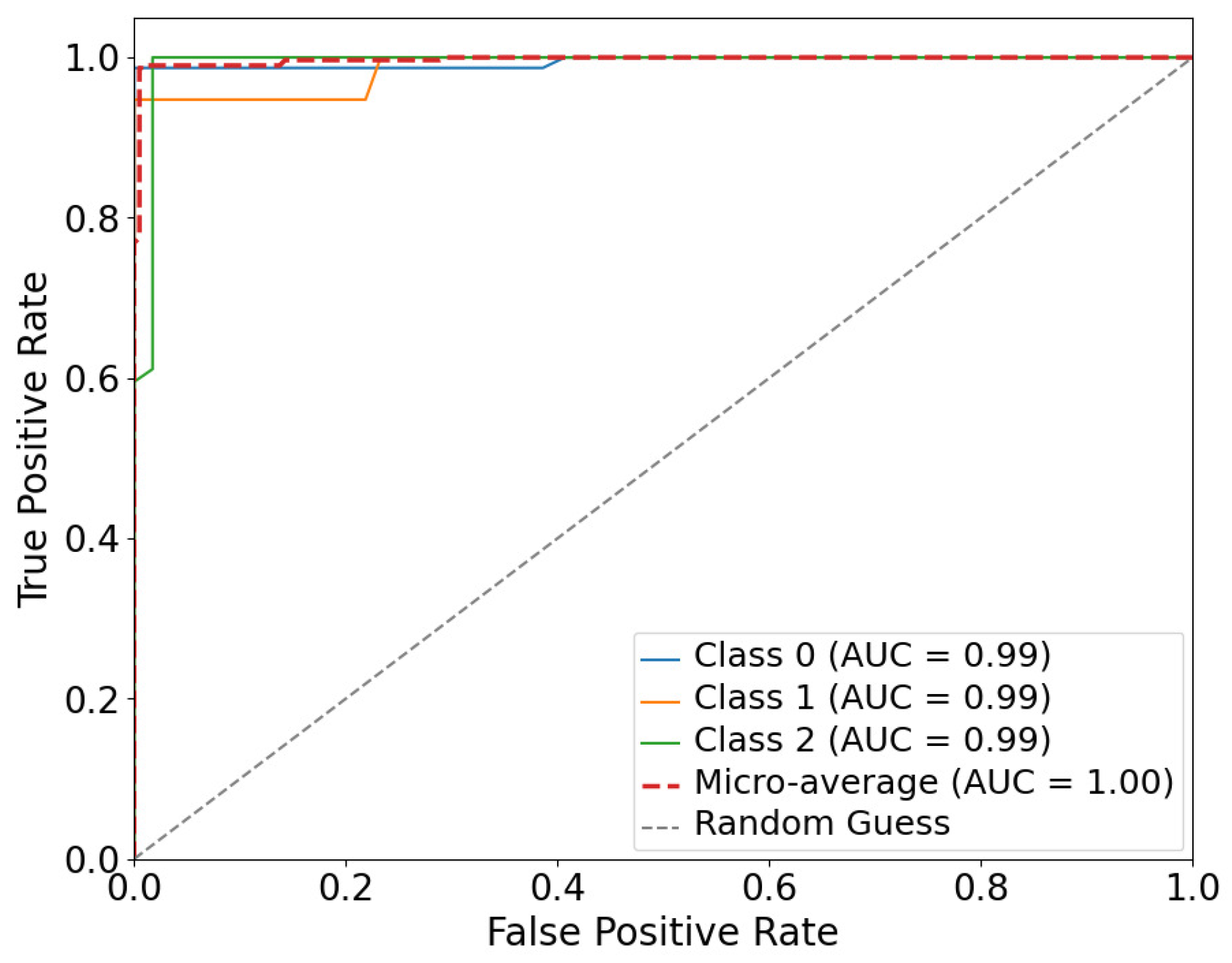
The classification models evaluate more than two classes. In this case, three classes (0, 1, and 2), represent Low, Medium, and High power outputs, respectively. As presented in Figure 11, the SVM with the RBF kernel curve shows the area under the curve (AUC) for each class, indicating how well the model is at distinguishing between classes. Class 0, Class 1, and Class 2 have an AUC of 0.99, which indicates that all three classes are distinguished by the model. The micro-average or the average ROC curve that considers the performance across all classes shows an AUC of 1.00. The micro-average AUC being 1.00 suggests that the SVM with the RBF kernel performs exceptionally well across all classes. It is important to note that the specifics of the data and the task at hand determine the type of kernel that should be used with the SVM.

Since solar power generation often exhibits complex, non-linear patterns due to various factors, like weather conditions, time of day, and seasonal changes, then the SVM used with the RBF kernel, which is particularly effective at capturing non-linear relationships in the data, is a potentially effective approach for optimizing solar power prediction.

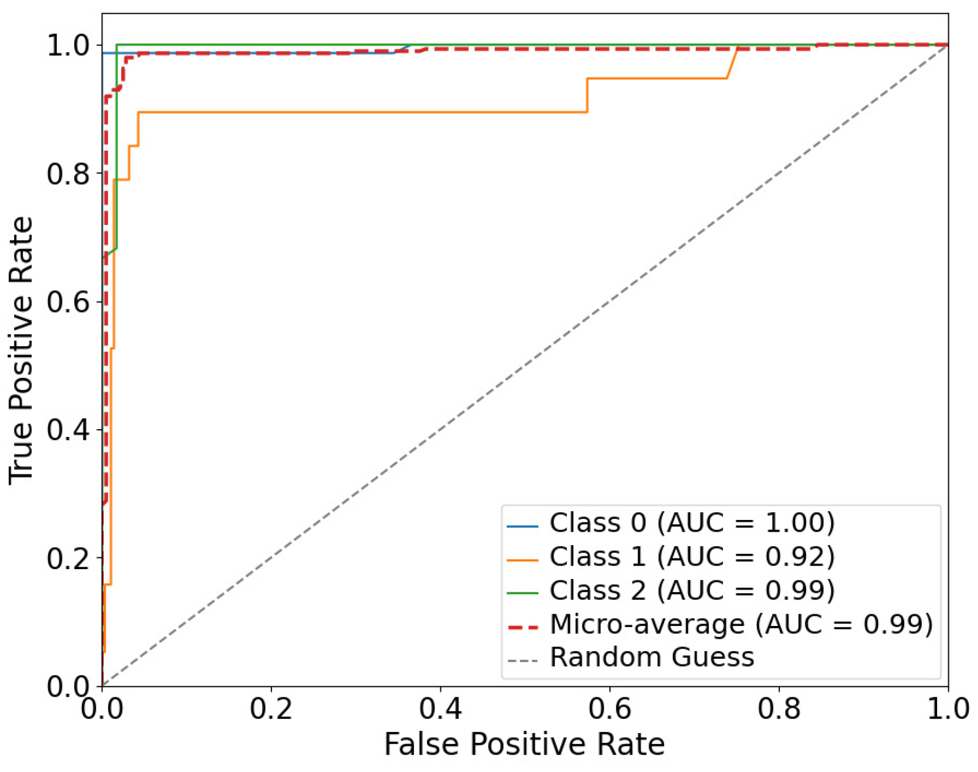
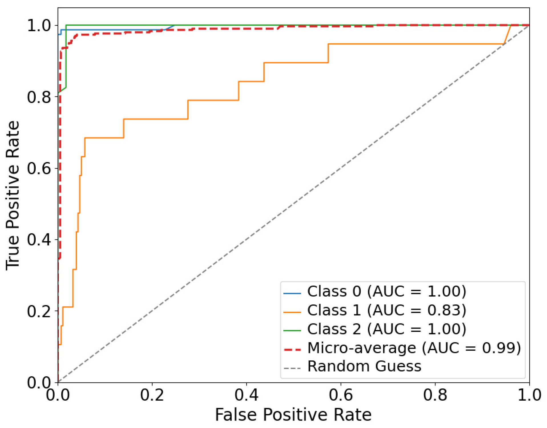
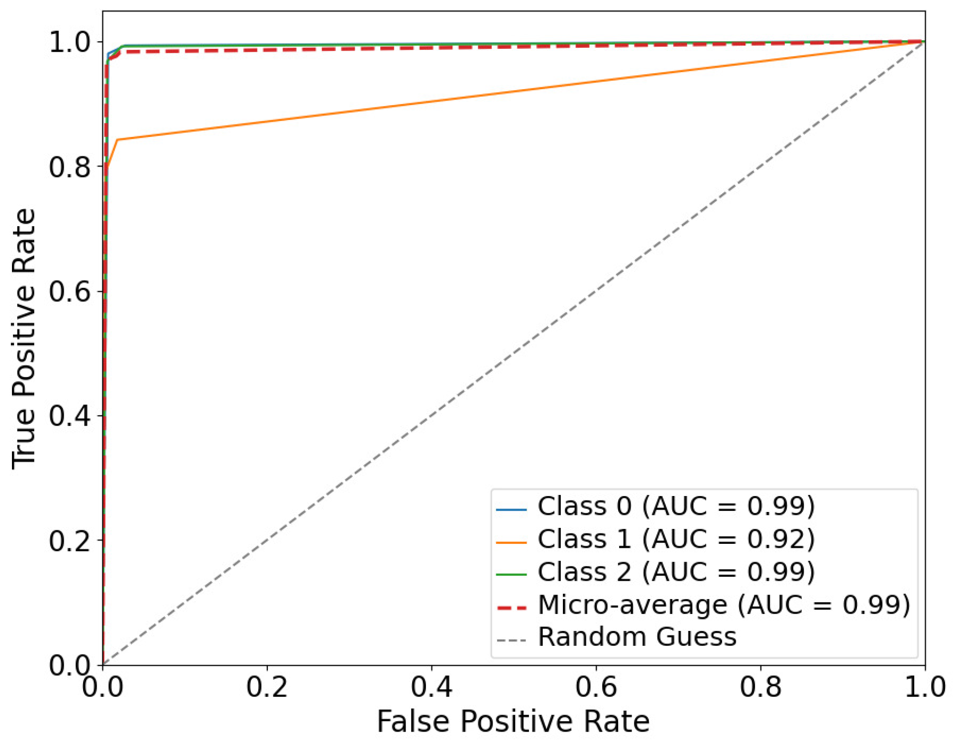
Figure 12 shows the SVM with the polynomial kernel curve shows AUCs of 1.00, 0.92, and 0.99 for Class 0, Class 1, and Class 2, respectively. The AUC of Class 1 shows that the SVM with the polynomial kernel is not as good as the SVM with the RBF kernel in distinguishing Class 1. 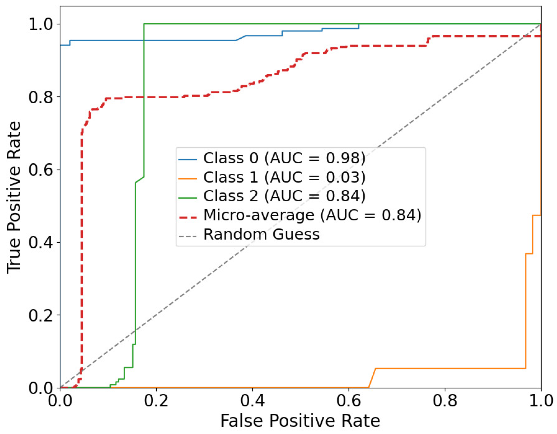The micro-average AUC of the SVM with the linear kernel is 0.99, which indicates that the model performs exceptionally well across all classes, as presented in Figure 13. The SVM with the linear kernel curve shows AUCs of 1.00, 0.83, and 1.00 for Class 0, Class 1, and Class 2, respectively. The AUC of Class 1 shows that the SVM with the linear kernel has a problem in distinguishing Class 1. The micro-average AUC of the SVM with the linear kernel is 0.99, which indicates that the model performs exceptionally well across all classes. The SVM with the sigmoid kernel curve, as depicted in Figure 14, shows AUCs of 0.98, 0.03, and 0.84 for Class 0, Class 1, and Class 2, respectively. The micro-average AUC of the SVM with the linear kernel is 0.84. These results show that the SVM with the sigmoid kernel has the poorest performance among the SVM models. Figure 15 illustrates the Decision Tree model which has a performance almost similar to that of the SVM with a polynomial kernel. The Deep Learning model shows AUCs of 0.99, 0.97, and 0.99 for Class 0, Class 1, and Class 2, respectively, as shown in Figure 16. The micro-average AUC of the Deep Learning model is 0.99. These results show that the Deep Learning model has a good performance in distinguishing between the classes.

5. Conclusions

The geographical location of Saudi Arabia and its dry weather made the kingdom a suitable place for constructing large-scale solar farm projects. The Sakaka PV power plant, the first of its kind in Saudi Arabia, has been operating and supplying 300 MW to the Saudi power grid since 2019. This paper compared six machine learning models to predict the output power of a solar PV farm. The support vector machine (SVM) with the RBF model shows the best performance among the other techniques. This method achieves accuracy = 98%, precision = 97%, recall = 96%, and F1 measure = 96%. The ROC curves show that the SVM with the RBF kernel is the best model with exceptional performance in distinguishing between the three classes, with a near-perfect classification ability as indicated by the high AUC values. On the other hand, the SVM with the sigmoid kernel has the poorest performance within the SVM models.

References

1. Ibrahim, N.F.; Mahmoud, M.M.; Alnami, H.; Mbadjoun Wapet, D.E.; Ardjoun, S.A.E.M.; Mosaad, M.I.; Hassan, A.M.; Abdelfattah, H. A new adaptive MPPT technique using an improved INC algorithm supported by fuzzy self-tuning controller for a grid-linked photovoltaic system. PLoS ONE 2023, 18, e0293613. [Google Scholar] [CrossRef] [PubMed]
2. Turai, T.; Ballard, I.; Rob, R. Short-term electrical load demand forecasting using artificial neural networks for off-grid distributed generation applications. In Proceedings of the 2017 Saudi Arabia Smart Grid (SASG), Jeddah, Saudi Arabia, 12–14 December 2017; IEEE: Piscataway, NJ, USA, 2017; pp. 1–7. [Google Scholar]
3. (SAMA), Saudi Central Bank Electricity Consumption by Sectors, Sourced from Publisher via KAPSARC Dataportal. 2019. Available online: https://datasource.kapsarc.org/pages/home/ (accessed on 12 November 2023).
4. Saudi Arabia Vision 2030. Available online: https://www.vision2030.gov.sa/media/rc0b5oy1/saudi_vision203.pdf (accessed on 12 December 2023).
5. Khan, K.A.; Quamar, M.M.; Al-Qahtani, F.H.; Asif, M.; Alqahtani, M.; Khalid, M. Smart grid infrastructure and renewable energy deployment: A conceptual review of Saudi Arabia. Energy Strategy Rev. 2023, 50, 101247. [Google Scholar] [CrossRef]
6. Abdalla, O.H.; Mostafa, A.A. Technical Requirements for Connecting Solar Power Plants to Electricity Networks. In Innovation in Energy Systems; IntechOpen: London, UK, 2019; p. 25. [Google Scholar]
7. Ahmed, R.; Sreeram, V.; Mishra, Y.; Arif, M. A review and evaluation of the state-of-the-art in PV solar power forecasting: Techniques and optimization. Renew. Sustain. Energy Rev. 2020, 124, 109792. [Google Scholar] [CrossRef]
8. Zhang, M.; Zhen, Z.; Liu, N.; Zhao, H.; Sun, Y.; Feng, C.; Wang, F. Optimal Graph Structure Based Short-Term Solar PV Power Forecasting Method Considering Surrounding Spatio-Temporal Correlations. IEEE Trans. Ind. Appl. 2023, 59, 345–357. [Google Scholar] [CrossRef]
9. Chu, Y.; Urquhart, B.; Gohari, S.M.; Pedro, H.T.; Kleissl, J.; Coimbra, C.F. Short-term reforecasting of power output from a 48 MWe solar PV plant. Sol. Energy 2015, 112, 68–77. [Google Scholar] [CrossRef]
10. Zhang, Y.; Beaudin, M.; Taheri, R.; Zareipour, H.; Wood, D. Day-ahead power output forecasting for small-scale solar photovoltaic electricity generators. IEEE Trans. Smart Grid 2015, 6, 2253–2262. [Google Scholar] [CrossRef]
11. Raza, M.Q.; Mithulananthan, N.; Li, J.; Lee, K.Y.; Gooi, H.B. An ensemble framework for day-ahead forecast of PV output power in smart grids. IEEE Trans. Ind. Inform. 2018, 15, 4624–4634. [Google Scholar] [CrossRef]
12. Wan, C.; Zhao, J.; Song, Y.; Xu, Z.; Lin, J.; Hu, Z. Photovoltaic and solar power forecasting for smart grid energy management. Csee J. Power Energy Syst. 2015, 1, 38–46. [Google Scholar] [CrossRef]
13. Prema, V.; Bhaskar, M.S.; Almakhles, D.; Gowtham, N.; Rao, K.U. Critical Review of Data, Models and Performance Metrics for Wind and Solar Power Forecast. IEEE Access 2021, 10, 667–688. [Google Scholar] [CrossRef]
14. Massidda, L.; Marrocu, M. Use of multilinear adaptive regression splines and numerical weather prediction to forecast the power output of a PV plant in Borkum, Germany. Sol. Energy 2017, 146, 141–149. [Google Scholar] [CrossRef]
15. Yan, K.; Du, Y.; Ren, Z. MPPT perturbation optimization of photovoltaic power systems based on solar irradiance data classification. IEEE Trans. Sustain. Energy 2018, 10, 514–521. [Google Scholar] [CrossRef]
16. Mellit, A.; Pavan, A.M.; Lughi, V. Short-term forecasting of power production in a large-scale photovoltaic plant. Sol. Energy 2014, 105, 401–413. [Google Scholar] [CrossRef]
17. Behera, M.K.; Majumder, I.; Nayak, N. Solar photovoltaic power forecasting using optimized modified extreme learning machine technique. Eng. Sci. Technol. Int. J. 2018, 21, 428–438. [Google Scholar] [CrossRef]
18. Huang, C.; Wang, L.; Lai, L.L. Data-driven short-term solar irradiance forecasting based on information of neighboring sites. IEEE Trans. Ind. Electron. 2018, 66, 9918–9927. [Google Scholar] [CrossRef]
19. Eseye, A.T.; Zhang, J.; Zheng, D. Short-term photovoltaic solar power forecasting using a hybrid Wavelet-PSO-SVM model based on SCADA and Meteorological information. Renew. Energy 2018, 118, 357–367. [Google Scholar] [CrossRef]
20. Srivastava, S.; Lessmann, S. A comparative study of LSTM neural networks in forecasting day-ahead global horizontal irradiance with satellite data. Sol. Energy 2018, 162, 232–247. [Google Scholar] [CrossRef]
21. Wang, H.; Yi, H.; Peng, J.; Wang, G.; Liu, Y.; Jiang, H.; Liu, W. Deterministic and probabilistic forecasting of photovoltaic power based on deep convolutional neural network. Energy Convers. Manag. 2017, 153, 409–422. [Google Scholar] [CrossRef]
22. Nejati, M.; Amjady, N. A New Solar Power Prediction Method Based on Feature Clustering and Hybrid-Classification-Regression Forecasting. IEEE Trans. Sustain. Energy 2021, 13, 1188–1198. [Google Scholar] [CrossRef]
23. Başaran, K.; Bozyiğit, F.; Siano, P.; Yıldırım Taşer, P.; Kılınç, D. Systematic literature review of photovoltaic output power forecasting. IET Renew. Power Gener. 2020, 14, 3961–3973. [Google Scholar] [CrossRef]
24. Shi, J.; Lee, W.J.; Liu, Y.; Yang, Y.; Wang, P. Forecasting power output of photovoltaic systems based on weather classification and support vector machines. IEEE Trans. Ind. Appl. 2012, 48, 1064–1069. [Google Scholar] [CrossRef]
25. Pan, M.; Li, C.; Gao, R.; Huang, Y.; You, H.; Gu, T.; Qin, F. Photovoltaic power forecasting based on a support vector machine with improved ant colony optimization. J. Clean. Prod. 2020, 277, 123948. [Google Scholar] [CrossRef]
26. Sharadga, H.; Hajimirza, S.; Balog, R.S. Time series forecasting of solar power generation for large-scale photovoltaic plants. Renew. Energy 2020, 150, 797–807. [Google Scholar] [CrossRef]
27. Dewangan, C.L.; Singh, S.; Chakrabarti, S. Combining forecasts of day-ahead solar power. Energy 2020, 202, 117743. [Google Scholar] [CrossRef]
28. Bellini, E. Saudi Arabia’s 300 MW Sakaka Solar Plant Comes Online. Available online: http://www.acwapower.com/en/projects/sakaka-pv-ipp/ (accessed on 14 June 2019).
29. Shah, A.A.; Ahmed, K.; Han, X.; Saleem, A. A Novel Prediction Error-Based Power Forecasting Scheme for Real PV System Using PVUSA Model: A Grey Box-Based Neural Network Approach. IEEE Access 2021, 9, 87196–87206. [Google Scholar] [CrossRef]
30. Balabel, A.; Alwetaishi, M.; Abdelhafiz, A.; Issa, U.; Sharaky, I.; Shamseldin, A.; Al-Surf, M.; Al-Harthi, M. Potential of Solatube technology as passive daylight systems for sustainable buildings in Saudi Arabia. Alex. Eng. J. 2022, 61, 339–353. [Google Scholar] [CrossRef]
Figure 1. Total power consumption in Saudi Arabia.
Energies 17 00525 g001
Figure 2. The consumed power in giga watt hour (GWh).
Energies 17 00525 g002
Figure 3. The 300 MW Sakaka PV project.
Energies 17 00525 g003
Figure 4. The percentage of the average output power generated by the solar farm for each season.
Energies 17 00525 g004
Figure 5. The average output power for each month generated by the solar farm.
Energies 17 00525 g005
Figure 6. Solar farm output power vs time for one day in summer, fall, winter, and spring (clear day).
Energies 17 00525 g006
Figure 7. Irradiance vs time for one day in summer, fall, winter, and spring (clear day).
Energies 17 00525 g007
Figure 8. Irradiance vs time for one day in summer, fall, winter, and spring (rainy or cloudy day).
Energies 17 00525 g008
Figure 9. Solar farm output power vs time for one day in summer, fall, winter, and spring (rainy or cloudy day).
Energies 17 00525 g009
Figure 10. The structure of the proposed prediction model.
Energies 17 00525 g010
Figure 11. ROC curve for multi-class classification using the SVM with the RBF kernel.
Energies 17 00525 g011
Figure 12. ROC curve for multi-class classification using the SVM with the polynomial kernel.
Energies 17 00525 g012
Figure 13. ROC curve for multi-class classification using the SVM with the linear kernel.
Energies 17 00525 g013
Figure 14. ROC curve for multi-class classification using the SVM with the sigmoid kernel.
Energies 17 00525 g014
Figure 15. ROC curve for multi-class classification using the Decision Tree model.
Energies 17 00525 g015
Figure 16. ROC curve for multi-class classification using the Deep Learning model.
Energies 17 00525 g016