Mutual Inductance Estimation of SS-IPT System through Time-Domain Modeling and Nonlinear Least Squares

Abstract

Inductive power transfer (IPT) systems are pivotal in various applications, relying heavily on the accurate estimation of mutual inductance to enable system interoperability discrimination and optimal efficiency tracking control. This paper introduces a novel mutual inductance estimation method for Series-Series IPT (SS-IPT) systems, utilizing time-domain modeling combined with nonlinear least squares. Initially, the time-domain model of SS-IPT systems is developed by deriving its ordinary differential equations (ODEs). Subsequently, the mutual inductance is estimated directly from these ODEs using a nonlinear least-squares approach. This approach necessitates only primary-side information, eliminating the need for communication, supplementary equipment, or frequency scanning. The simplicity and directness of using collected real-time data enhance the practical applicability of our approach. The effectiveness of the proposed method is substantiated through simulations and experimental data. Results demonstrate that the estimation accuracy of our method remains more than 95.0% in simulations and more than 92.5% in experimental data.

1. Introduction

Inductive power transfer (IPT) systems are promising technologies to create safer, more efficient, and clutter-free power solutions. IPT systems have been extensively utilized in diverse applications, like electric vehicle charging and industrial automation [1,2,3]. Mutual inductance of IPT systems is usually required to enable system interoperability discrimination [4] and optimal efficiency tracking control [5]. However, in practice, mutual inductance may be changed due to the misalignment between transmitting and receiving coils [6]. Hence, mutual inductance estimation is crucial to technology in IPT systems for their optimal performance.

Currently, most methods to estimate mutual inductance in IPT systems are based on frequency-domain analysis. These frequency-domain methods are to estimate mutual inductance by solving the system of equations based on KCL and KVL in a frequency domain. Typically, the method in [7] can estimate mutual inductance by using input voltage and voltage at only one operating frequency for an SS-IPT system. However, this method will fail when the system operates at the resonant frequency, and it can be used to measure mutual inductance offline. Methods in [8,9,10] overcome the shortcoming in [7] and can estimate mutual inductance accurately online. However, their performance heavily relies on several parameters such as the resistor of output and the parasitic resistor of the inductor. With similar processes in [7,8,9,10], additional circuits or coils can be designed to get more information from IPT systems to help improve the performance of the estimation results [11,12]. Obviously, additional circuits or coils will increase the system’s cost and complexity. Without additional components, more information of the systems can be extracted by conducting a frequency sweeping [13,14,15,16]. In [13], by selecting two operating frequencies greater than the resonant frequency of the secondary circuit, and establishing the equations of the system in each operating frequency, the mutual inductance was calculated for an SS-IPT with a passive rectifier. Similarly, with the sweeping frequency processes, mutual inductance in the IPT systems with active rectifiers could also be well estimated [14,15,16]. However, frequency sweeping methods regard the loads of IPT systems as a constant equivalent resistor, which may lead to poor accuracy since the loads of IPT systems vary at different operating frequencies. Furthermore, during frequency sweeping, IPT systems have to work in abnormal conditions. Different from frequency sweeping, harmonics analysis methods extract information at a certain operation frequency by making full use of harmonic components in the signals [17,18,19]. In [17], fundamental and third harmonic components of input current and input voltage were used to estimate mutual inductance in an SS-IPT system. In [18,19], tapered harmonics were used. Although harmonic components have been proven to enhance estimation accuracy, they cannot be measured accurately, and the measured error generally leads to poor estimation. Recently, with the development of artificial intelligence, data-driven methods have been utilized to estimate mutual inductance with frequency-domain analysis. In [20], harmonic components of current and voltage in the primary sides were used to estimate mutual inductance by using a random forest algorithm. A digital twin technology with a particle swarm optimization algorithm was applied to calculate mutual inductance by fitting the current in the primary side [21].

Based on the analysis above, several limitations of frequency-domain mutual inductance estimation methods can be identified. Firstly, incorporating additional auxiliary devices could lead to increased costs. Secondly, methods that require frequency sweeping may compromise accuracy due to the variability of the equivalent load across different frequencies. Additionally, frequency sweeping cannot be utilized in online applications. Thirdly, frequency-domain decomposition techniques often struggle to accurately capture high-order harmonic components, which are crucial for these approaches. In contrast, time-domain analysis offers a more intuitive and straightforward interpretation, is well-suited for real-time applications, and preserves the chronological integrity of the data. However, research on using time-domain methods for mutual inductance identification remains limited. In this paper, we propose a mutual inductance estimation method for Series-Series IPT (SS-IPT) based on a time-domain model and nonlinear least squares. A detailed description of the mutual inductance estimation method is presented in Section 2. Section 3 validates the proposed method with simulation data, and Section 4 further verifies it through experimental data. Conclusions are drawn in Section 5.

2. Mutual Inductance Estimation of SS-IPT Systems

2.1. Configuration and Equivalent Circuit of SS-IPT

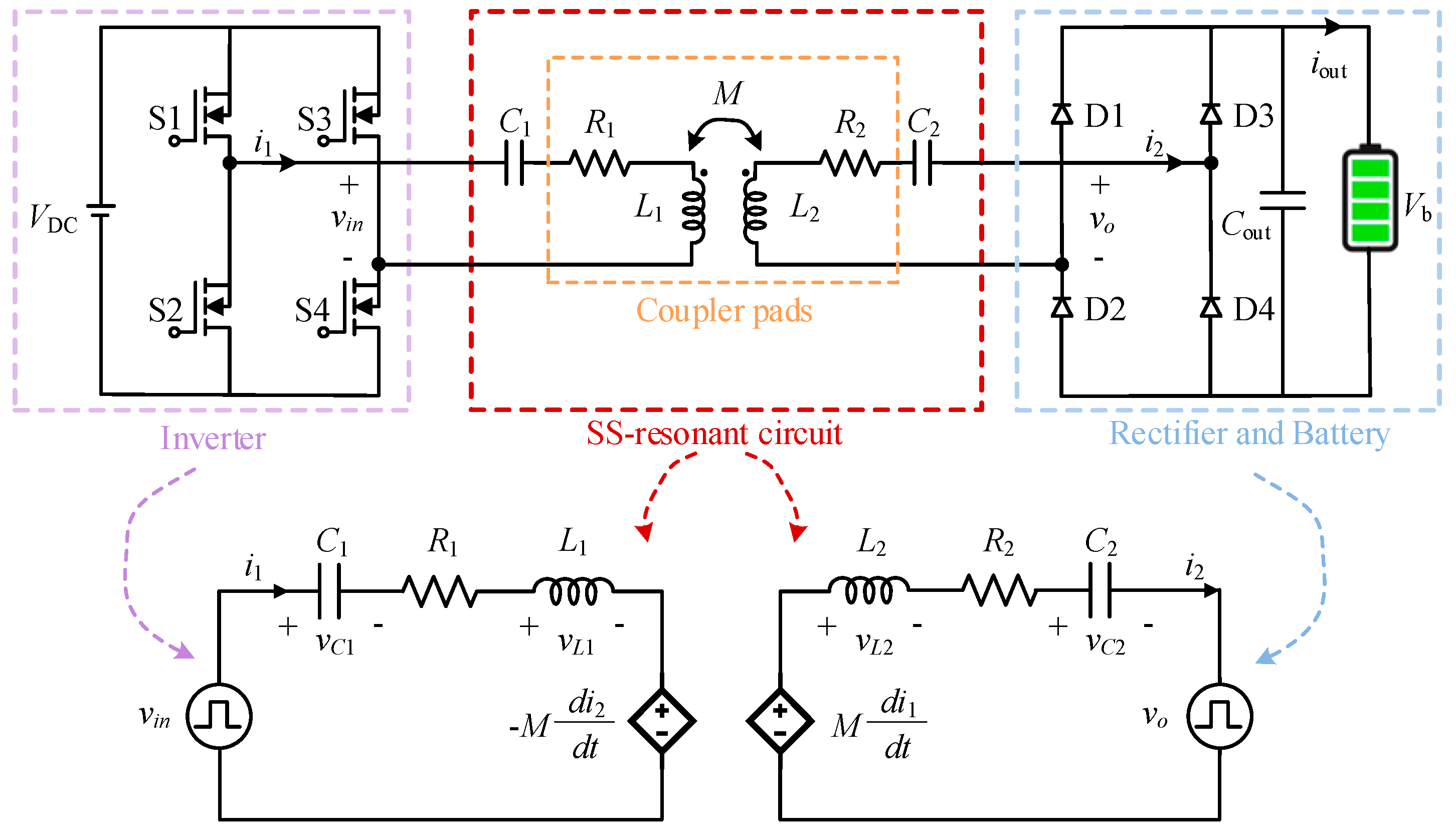
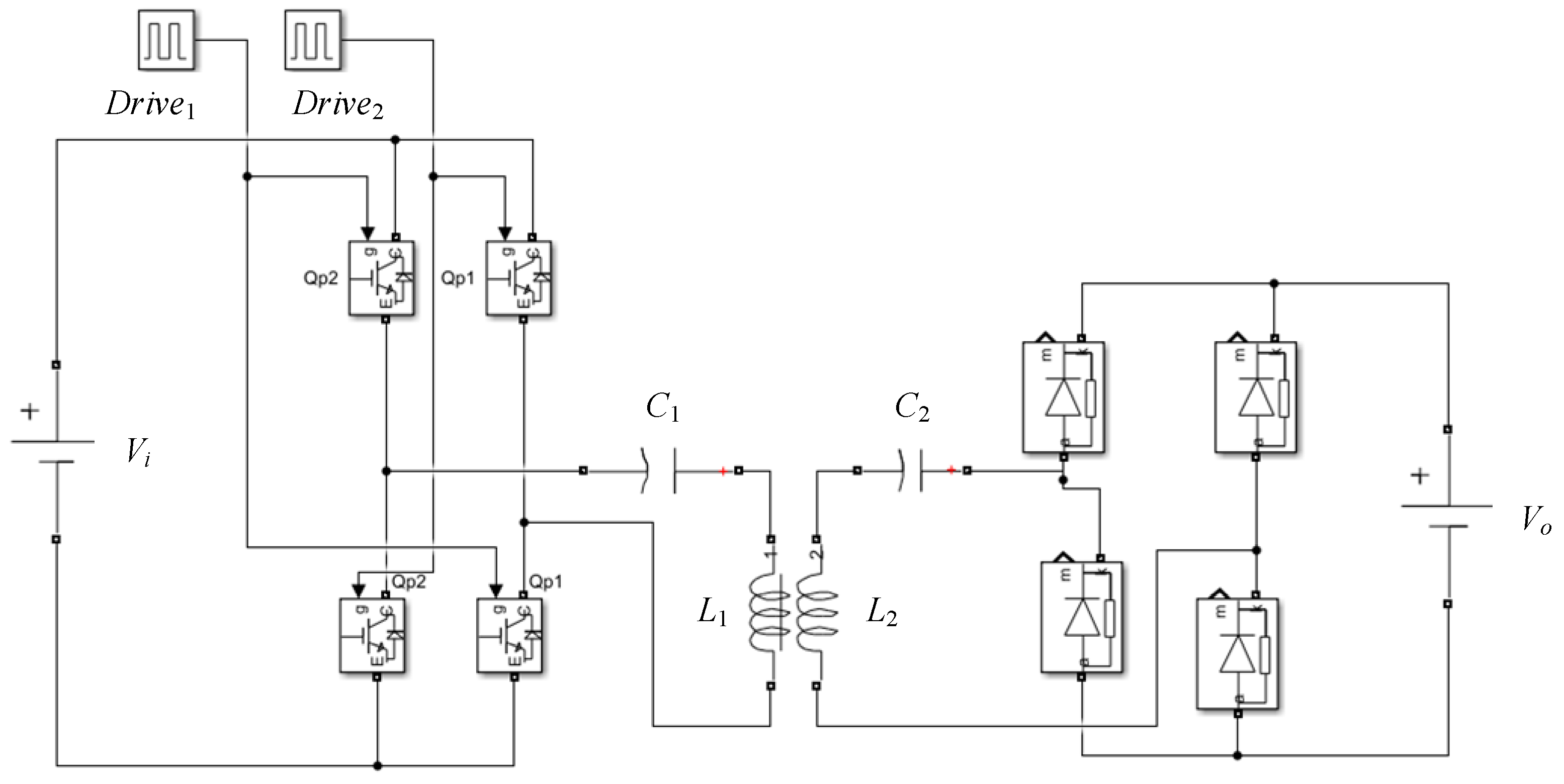
As shown in Figure 1, the main components of the SS-IPT system include a full-bridge inverter, an SS resonant circuit, a full-bridge rectifier, and a battery load. The inverter converts the DC power into AC power with a square waveform. The SS resonant circuit refers to the arrangement where both the transmitter and receiver coils are connected in series with a capacitor. With the output of the inverter, the SS resonant circuit will transfer power from the transmitter to the receiver via magnetic coupling. The full-bridge rectifier converts the output of the SS resonant circuit into DC power to charge the battery.

Figure 1. Configuration of SS-IPT system and its equivalent circuit.

The equivalent circuit of the above system is also shown in Figure 1. The excitation square source v_in is utilized to replace the inverter as the input, and values of v_in will alternate between +V_DC and −V_DC. With a similar approach, the rectifier and battery load can be considered as another square source v_o whose values are switched between +V_b and −V_b. For the SS resonant circuit, a transformer model is used. In the equivalent circuit, L₁ and L₂ are the self-inductance of the transmitting and receiving coils, respectively. R₁ and R₂ are the resistance of the two coils. C₁ and C₂ are the series resonant capacitors connecting to the transmitting and receiving coils, respectively. M is the mutual inductance between the two coils. Current i₁ and i₂ are the input and output current, respectively.

2.2. Time-Domain SS-IPT Model

With the equivalent circuit in Figure 1, the SS-IPT system can be described by the following time-domain KVL equations in (1). In this equation, any variable x represents x(ωt) and the derivative order of variables is recorded in the superscript. ω is the operating angular frequency, and it can be easily calculated from the operating frequency f_w by using ω = 2πf_w.

$$\left\{\begin{array}{l}{v}_{in}-v_{L1}-v_{C1}-i_1{R}_1+\omega {Mi}_2^{(1)}=0\\ v_o+v_{L2}+v_{C2}+i_2{R}_2-\omega {Mi}_1^{(1)}=0\end{array}\right.$$

(1)

On the basis of the characteristics of inductors, the voltage across L₁ and L₂ and the current through them should satisfy (2). Similarly, the voltage and current of C₁ and C₂ should satisfy (3).

$$\left\{\begin{array}{l}{v}_{L1}=\omega L_1{i}_1^{(1)}\\ v_{L2}=\omega L_2{i}_2^{(1)}\end{array}\right.$$

(2)

$$\left\{\begin{array}{l}{i}_1=\omega C_1{v}_{C1}^{(1)}\\ i_2=\omega C_2{v}_{C2}^{(1)}\end{array}\right.$$

(3)

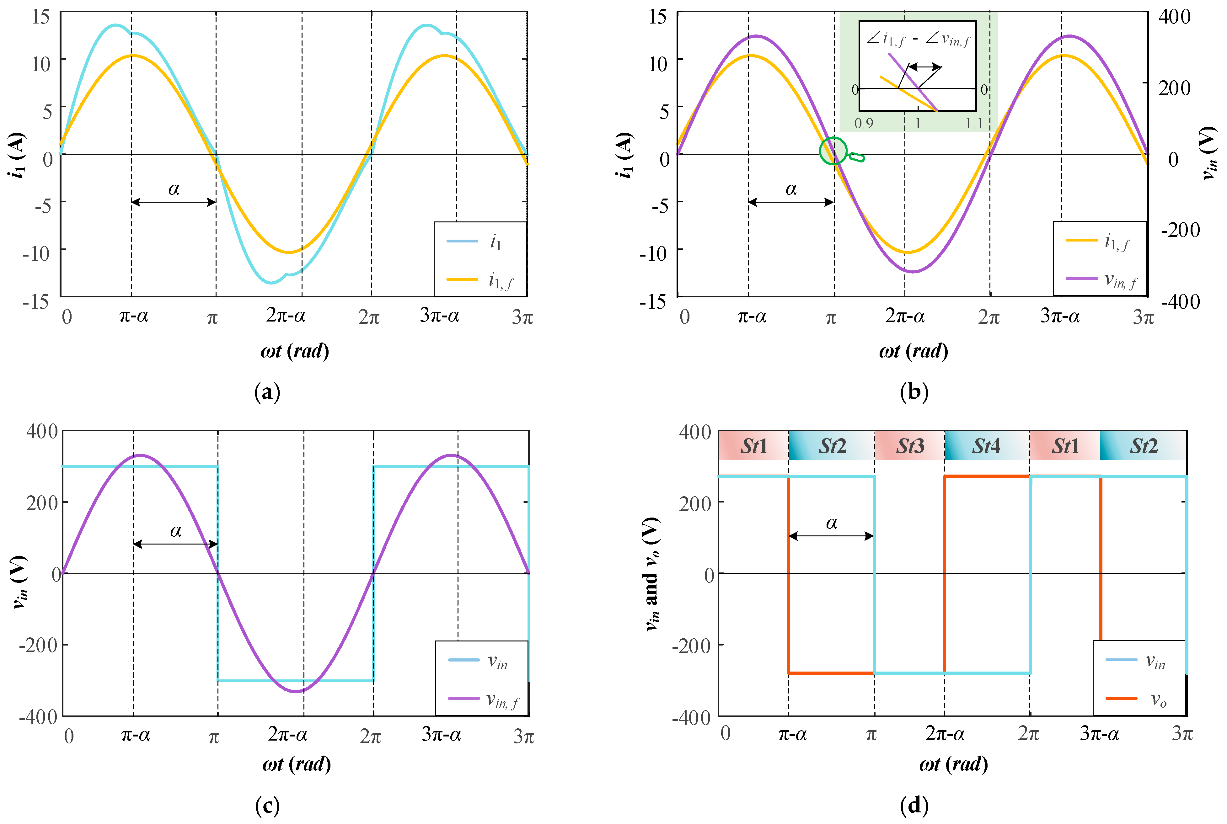
By differentiating (1) three times, equations with four-order derivatives can be obtained in (4) and (5). By substituting (2) and (3) into (4) and (5) to eliminate i₂ and its corresponding derivatives, the time-domain ordinary differential equation (ODE) in (6) is deduced. Coefficients a₄~a₀, b₃~b₁, and c₃ in (6) are given in (7) and (8). Nonzero coefficients b₃~b₁ and c₃ complicate the ODE since the nonlinear dynamics of v_in and v_o are considered. Fortunately, ODE in (6) can be simplified according to the features of v_in and v_o. As shown in Figure 2d, any working cycle of SS-IPT systems can be divided into four stages (St1~St4), and values of v_in and v_o maintain a constant level in each stage. Therefore, derivatives of v_in and v_o will be zeros in each stage, and ODE in (6) can be simplified in (9) [22]. The division of stages is determined by the phase angle α between v_in and v_o in Figure 2d, and α can be calculated by the phase difference between the fundamental components of i₁ and v_in [23] as illustrated in (10). For example, the fundamental components of i₁ and v_in are shown in Figure 2a,c, and angle α is determined in Figure 2b.

$$\left\{\begin{array}{l}{v}_{in}^{(1)}-v_{L1}^{(1)}-v_{C1}^{(1)}-i_1^{(1)}{R}_1+\omega {Mi}_2^{(2)}=0\\ v_{in}^{(2)}-v_{L1}^{(2)}-v_{C1}^{(2)}-i_1^{(2)}{R}_1+\omega {Mi}_2^{(3)}=0\\ v_{in}^{(3)}-v_{L1}^{(3)}-v_{C1}^{(3)}-i_1^{(3)}{R}_1+\omega {Mi}_2^{(4)}=0\end{array}\right.$$

(4)

$$v_o^{(3)}+v_{L2}^{(3)}+v_{C2}^{(3)}+i_2^{(3)}{R}_2-\omega M{i}_1^{(4)}=0$$

(5)

$${\left[\begin{array}{c}{a}_4\\ a_3\\ a_2\\ a_1\\ a_0\end{array}\right]}^T\left[\begin{array}{c}{i}_1^{(4)}\\ i_1^{(3)}\\ i_1^{(2)}\\ i_1^{(1)}\\ i_1\end{array}\right]={\left[\begin{array}{c}0\\ b_3\\ b_2\\ b_1\\ 0\end{array}\right]}^T\left[\begin{array}{c}{v}_{in}^{(4)}\\ v_{in}^{(3)}\\ v_{in}^{(2)}\\ v_{in}^{(1)}\\ v_{in}\end{array}\right]+{\left[\begin{array}{c}0\\ c_3\\ 0\\ 0\\ 0\end{array}\right]}^T\left[\begin{array}{c}{v}_o^{(4)}\\ v_o^{(3)}\\ v_o^{(2)}\\ v_o^{(1)}\\ v_o\end{array}\right]$$

(6)

$$\left\{\begin{array}{l}{a}_4=\omega L_1{L}_2-\omega M^2\\ a_3=L_1{R}_2+L_2{R}_1\\ a_2=\left(C_2{L}_2+C_1{L}_1+C_1{C}_2{R}_1{R}_2\right)/\omega C_1{C}_2\\ a_1=\left(C_1{R}_1+C_2{R}_2\right)/{\omega }^2{C}_1{C}_2\\ a_0=1/{\omega }^3{C}_1{C}_2\end{array}\right.$$

(7)

$$\left\{\begin{array}{l}{b}_3=-L_2,b_2=-R_2/\omega ,b_1={-1/\omega }^2{C}_2\\ c_3=M\end{array}\right.$$

(8)

$$\left\{\begin{array}{l}{a}_4{i}_1^{(4)}(\omega t)+a_3{i}_1^{(3)}(\omega t)+a_2{i}_1^{(2)}(\omega t)+a_1{i}_1^{(1)}(\omega t)+a_0{i}_1(\omega t)=0\\ \omega t\in st,\hspace{0.33em}st\in \{St1,St2,St3,St4\}\end{array}\right.$$

(9)

$$\alpha =\frac{\pi }{2}+(\angle i_{1,f}-\angle v_{in,f})$$

(10)

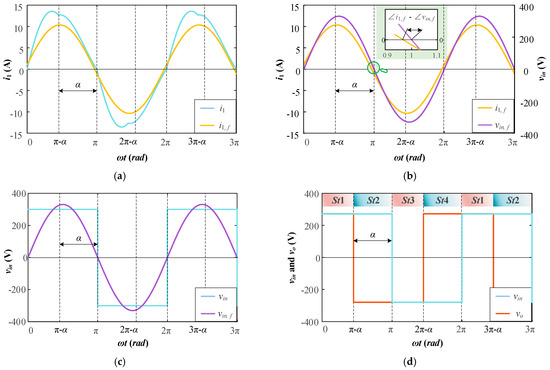
Figure 2. Simulation waveform of SS-IPT systems. (a) i₁ and its fundamental component. (b) Fundamental components of i₁ and v_in. (c) v_in and its fundamental component. (d) v_in and v_o.

2.3. Nonlinear Least Square

After the time-domain model of the SS-IPT system is established, nonlinear least squares (NLS) are used to determine the mutual inductance. NLS is an effective technique for estimating the parameters in models described by differential equations, including complex models such as differential equations in fields like physics, engineering, and biomechanics [24,25].

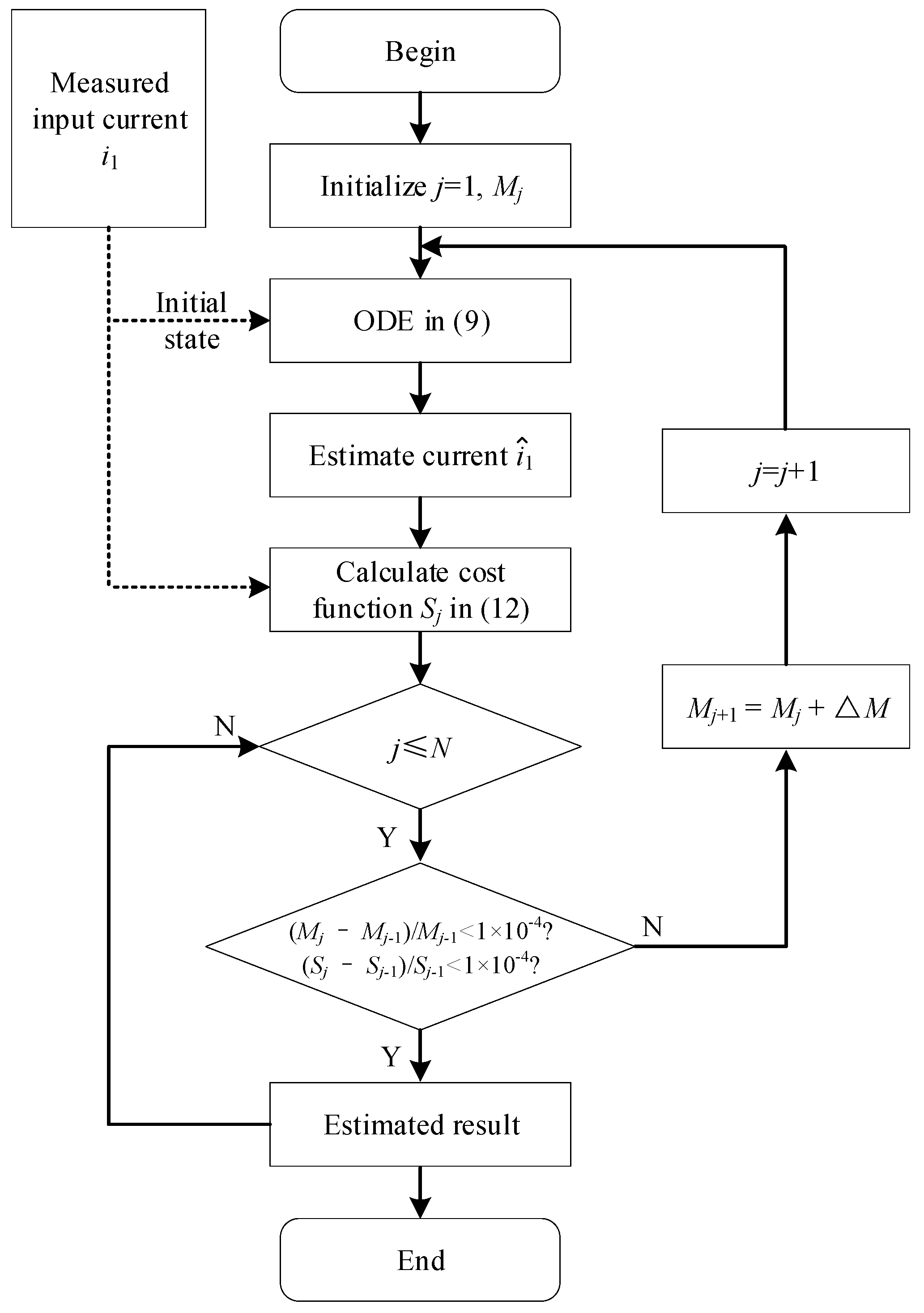
According to (9), let us consider a fourth-order differential equation of the form in (11). Now, the goal is to find the parameter M that minimizes the sum of squared residuals between observed data and the model predictions, and the cost function in NLS estimation can be expressed as (12). With the flowchart in Figure 3, the proposed mutual inductance estimation method can be summarized as the following steps:

Figure 3. Flowchart of the proposed mutual inductance estimation method.

• Step 1. Parameter Initialization: Initialize the current iteration index j = 1, and choose initial estimates for the mutual inductance M;
• Step 2. Numerical Integration: Use a four-order Runge–Kutta numerical solver to integrate the differential equation and compute ${\widehat{i}}_1$(wt, M_j);
• Step 3. Residual Computation: Compute the difference between observed data i₁ and model predictions ${\widehat{i}}_1$, and calculate the loss function by using (12);
• Step 4. Optimization: If the current iteration index j is less than the predefined maximum iteration count N and the relative change in the estimated mutual inductance or the cost function values between iterations is more than 1 × 10⁻⁴, then the mutual in the next iteration index will be updated using the formula M_j+1 = M_j + ∆M. This update will utilize a trust-region-reflective algorithm for NLS. Additionally, the iteration index j will be incremented by 1;
• Step 5. Convergence Verification: Repeat the optimization until the changes in the relative changes (M_j − M_j−1)/M_j−1 or (S_j − S_j−1)/S_j−1 are below 1 × 10⁻⁴, or j > N.

$$\left\{\begin{array}{l}{i}_1^{(4)}(\omega t)=F\left(i_1^{(3)}(\omega t),i_1^{(2)}(\omega t),i_1^{(1)}(\omega t);M\right)\\ \omega t\in st,\hspace{0.33em}st\in \{St1,St2,St3,St4\}\end{array}\right.$$

(11)

where F is the nonlinear function.

$$S(M)=\frac{1}{n}{\displaystyle {\sum }_{j=1}^n{\left(i_1\left(\omega t_j\right)-{\widehat{i}}_1\left(\omega t_j;M\right)\right)}^2}$$

(12)

where i₁(wt_j) is the observed values of input current at time t_j, and ${\widehat{i}}_1$(wt_j; M) is the input current obtained by solving the differential equation numerically.

3. Simulation

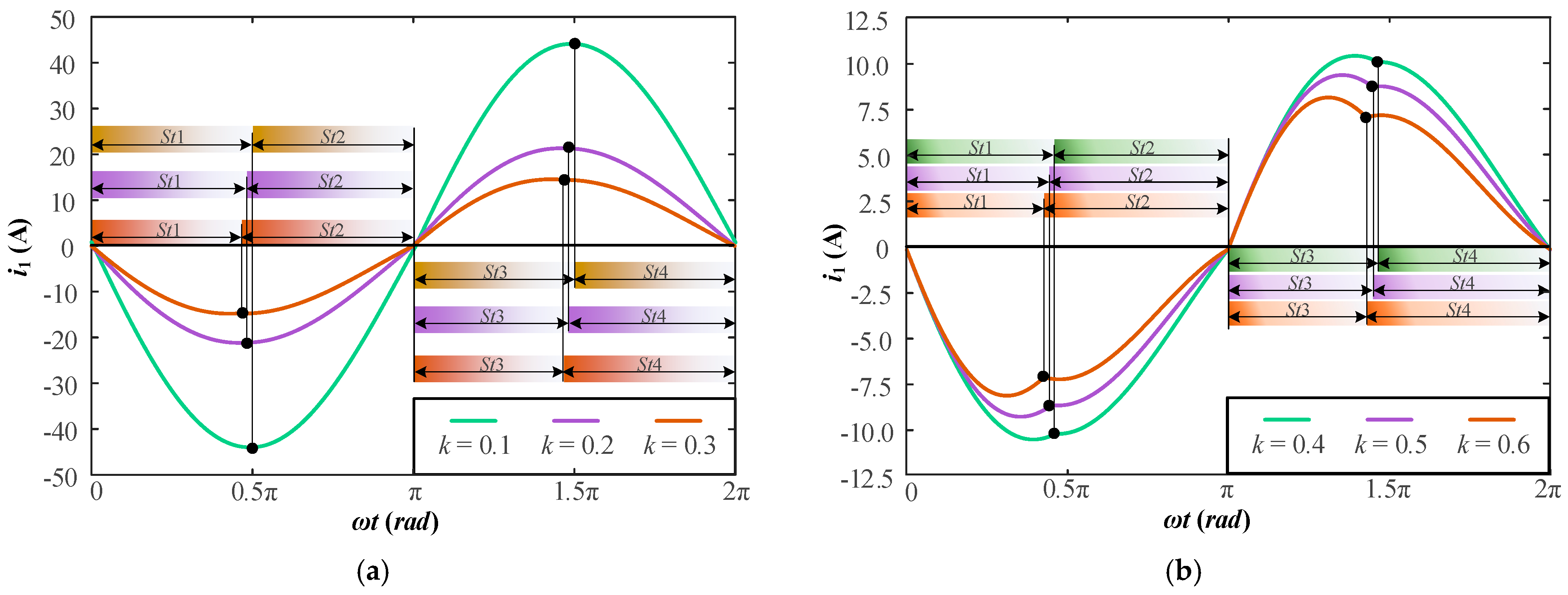
The proposed mutual inductance estimation method will be verified in a group of simulation data, which is generated from a model in Simulink, and the basic setup of the model is illustrated in Table 1. As shown in Table 1, parameters of the SS-IPT systems, including self-inductance of two coils L₁~L₂, the capacitance of resonant capacitors C₁~C₂, and parasitic resistance of two coils R₁~R₂, are given. With the above parameter, a Simulink model is established in Figure 4. With the simulation model, input current i₁ and input voltage v₁ of the transmitter-side under seven coupling coefficients k are measured, as shown in Figure 5. The coupling coefficients are determined in (13). On the basis of (11), i₁ in a period can always be divided into four stages St1~St4, and i₁ in each stage can be utilized to estimate mutual inductance. The waveforms of i₁ under different coupling coefficients are shown in Figure 5a,b. As shown in Figure 5a, with small coupling coefficients (k = 0.1 to 0.3), the distortion in the waveform of i₁ is progressively small and resembles a sine wave. However, when the coupling coefficient exceeds 0.3, the waveform begins to show detailed distortions, as illustrated in Figure 5b. This is because when the coupling coefficient increases, the impedance of the primary side for the fundamental frequency increases, while the impedance for higher harmonics decreases. As a result, the fundamental component of i₁ is reduced, and the higher harmonic components of i₁ are increased, ultimately leading to the distortion of i₁ waveform when the coupling coefficient increases.

Table 1. Setup of the SS-IPT simulation model.

Operating frequency fw	85 kHz
Sampling frequency fs	20 MHz
Self-inductance L1 and L2	56.67 μH, 57.23 μH
Capacitance of C1 and C2	61.52 nF, 60.90 nF
Parasitic resistance R1 and R2	0.036 Ω, 0.039 Ω
Coupling coefficient k	{0.10, 0.15, 0.20, …, 0.65}

Figure 4. Simulation model of SS-IPT system in Simulink.

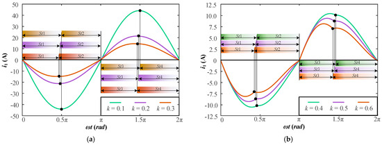
Figure 5. Input current i₁ of transmitter-side under different values of coupling coefficient k. (a) k = 0.1~0.3. (b) k = 0.4~0.6.

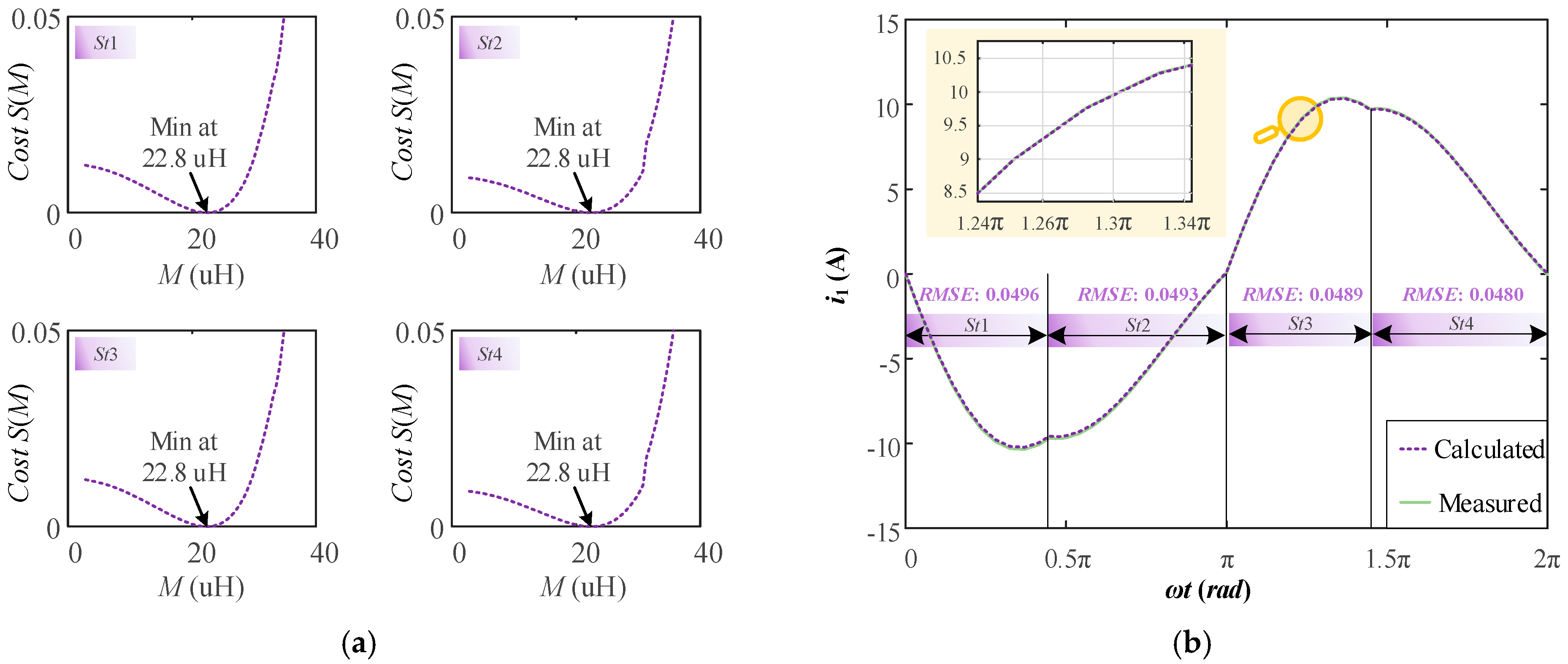
Each segment of the above simulation data is input into the proposed method to estimate the mutual inductance. Taking the simulation data under k = 0.4 as an example, the mutual inductance estimation results for stages St1 to St4 are shown in Figure 6a. Observation of Figure 6a reveals that in all four stages, St1 to St4, the NLS cost function S(M) finally converges at a minimum value. The value of M at which S(M) is minimized is used as the estimated mutual inductance, and the estimated mutual inductance for stages St1, St2, St3, and St4 are all 22.8 µH, which coincides exactly with the theoretical value 22.79 uH. To further analyze the estimated results, the calculated i₁ and measured i₁ from simulation data are compared in Figure 6b. It can be found that the calculated and measured i₁ are very close. According to (14), the root mean square error (RMSE) of measured i₁ and calculated i₁ in St1~St4 is 0.0496, 0.0493, 0.0489, and 0.0480, respectively. The average estimated mutual inductance M_ave is calculated in (15) to improve the stability of the results.

$$k=\frac{M}{\sqrt{L_1{L}_2}}$$

(13)

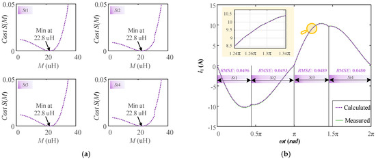
Figure 6. Mutual estimation results of the proposed method under k = 0.4. (a) Cost function under stages St1~St4. (b) Comparison between measured i₁ and calculated i₁ with estimated M.

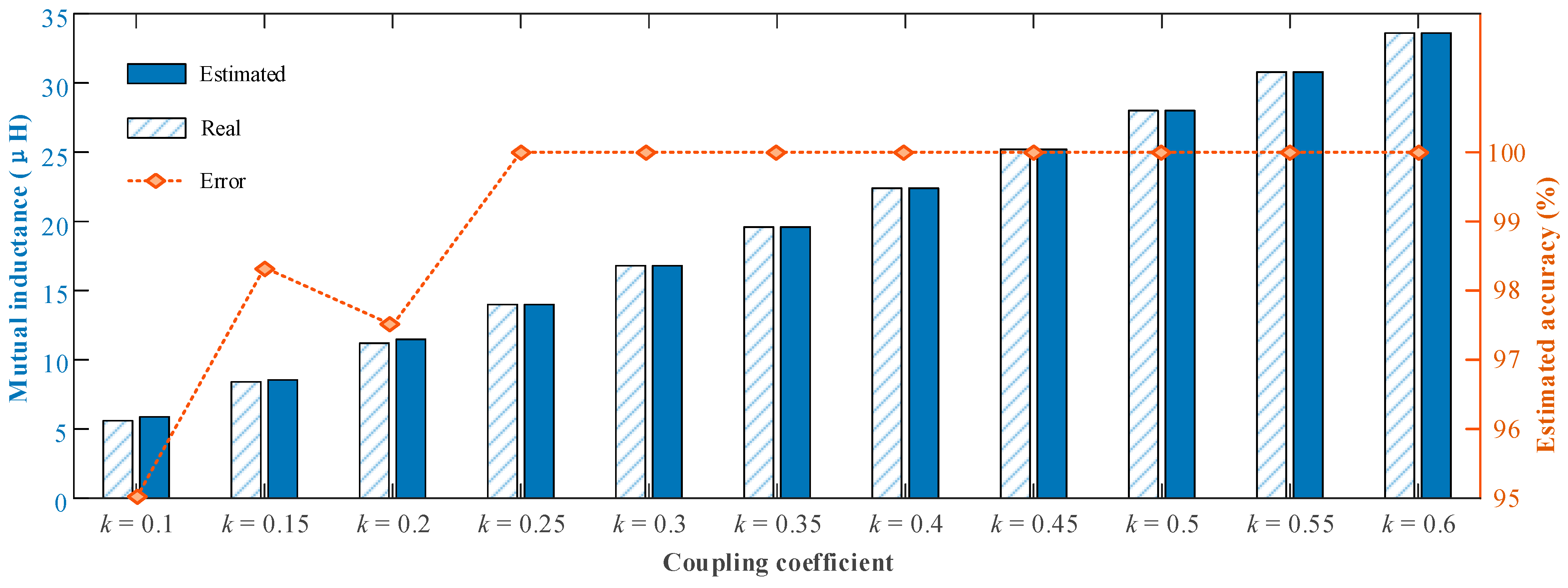
The estimated results are displayed in Figure 7. As illustrated in Figure 7, it is evident that the proposed method can accurately estimate mutual inductance across different coupling coefficients. When k > 0.25, the estimation accuracy approaches 100%. However, when k < 0.25, the accuracy begins to decline. This decrease in accuracy under weak coupling conditions can be attributed to the fact that small errors in mutual inductance estimation can lead to significant relative percentage errors. For example, when k = 0.01, the difference between the estimated and actual mutual inductance values is only 0.56 µH, yet this results in a 5% loss in relative accuracy. In summary, the simulated data show that the accuracies of the method proposed in this paper for k values ranging from 0.1 to 0.6 are greater than 95%, which indicates that the proposed method can estimate mutual inductance with high accuracy.

$$RMSE=\frac{1}{n}{\displaystyle \sum _{j=1}^n\sqrt{{\left(i_{1-measured}(\omega t_j)-i_{1-calculated}(\omega t_j)\right)}^2}}$$

(14)

$$M_{ave}=\frac{1}{4}\left(M_{est1}+M_{est2}+M_{est3}+M_{est4}\right)$$

(15)

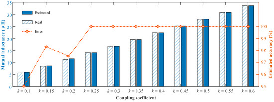
Figure 7. Estimated mutual inductance and the corresponding error under different coupling coefficients with simulation data.

4. Experiment

4.1. Experiment Setup

This section employs the proposed mutual inductance estimation method on experimental data to further affirm the effectiveness of the technique. Initially, an experiment prototype specifically designed for mutual inductance estimation is set up. The parameters of this prototype, including the self-inductance L₁~L₂ of both the transmitting and receiving coils, the capacitance of resonant capacitors C₁~C₂, parasitic resistance R₁~R₂, and the operating frequency f_w, are all identical to those used in the simulations shown in Table 1. The sampling frequency for the input current i₁ is fixed at 20 MHz, and both the input and output voltages are set to 100 V. With the above parameters, the experiment prototype is illustrated in Figure 8.

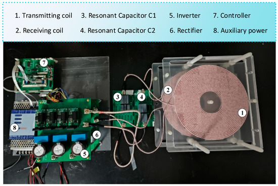
Figure 8. Experiment prototype for mutual inductance identification.

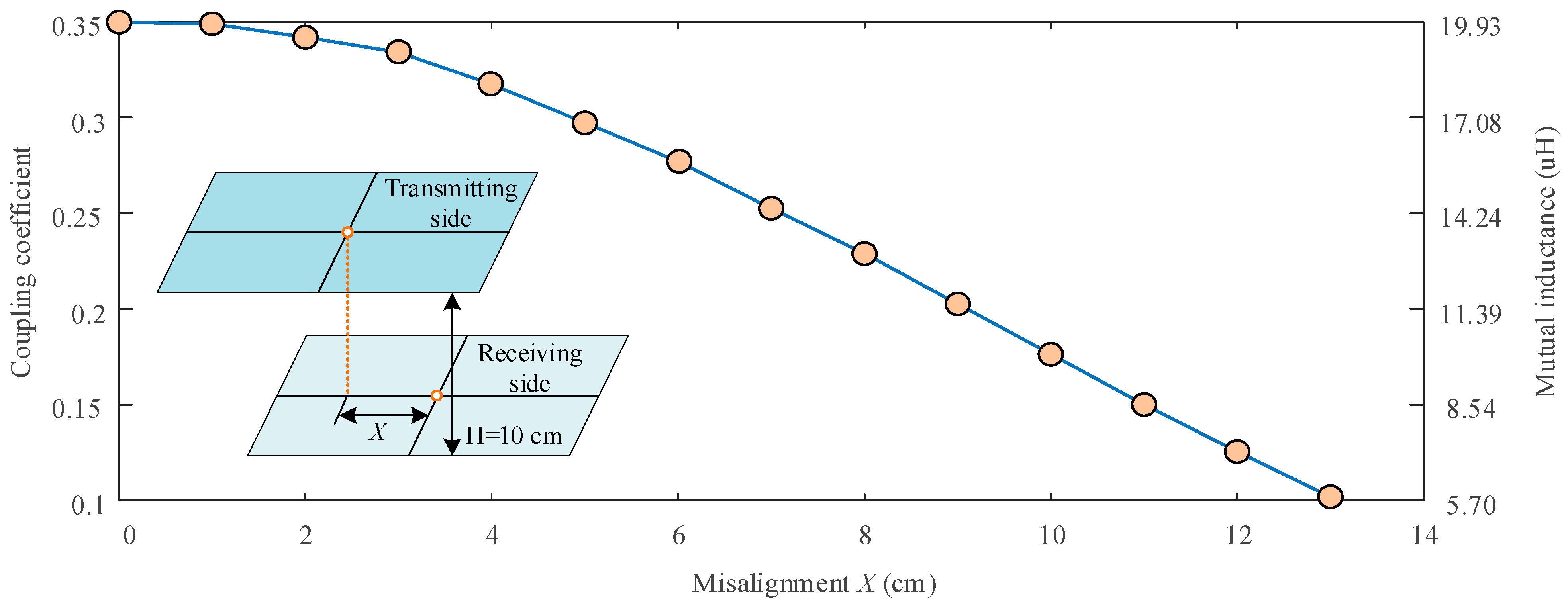
In this experimental configuration, the distance between the transmitting coil and the receiving coil is maintained at 10 cm. Additionally, their lateral misalignments, denoted as X, are meticulously measured. An LCR meter is employed to measure the mutual inductance at each specific misalignment. The findings are graphically represented in Figure 9. At a misalignment of X = 0 cm, the mutual inductance reaches its maximum at 19.93 μH, corresponding to a coupling coefficient of approximately 0.35. With the increasing misalignment, the mutual inductance will be reduced. As the misalignment increases to 13 cm, there is a noticeable decrease in mutual inductance to 5.70 μH, with the coupling coefficient diminishing to about 0.1.

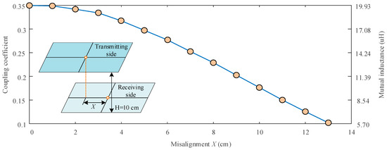
Figure 9. Coupling coefficients and mutual inductance under different misalignments.

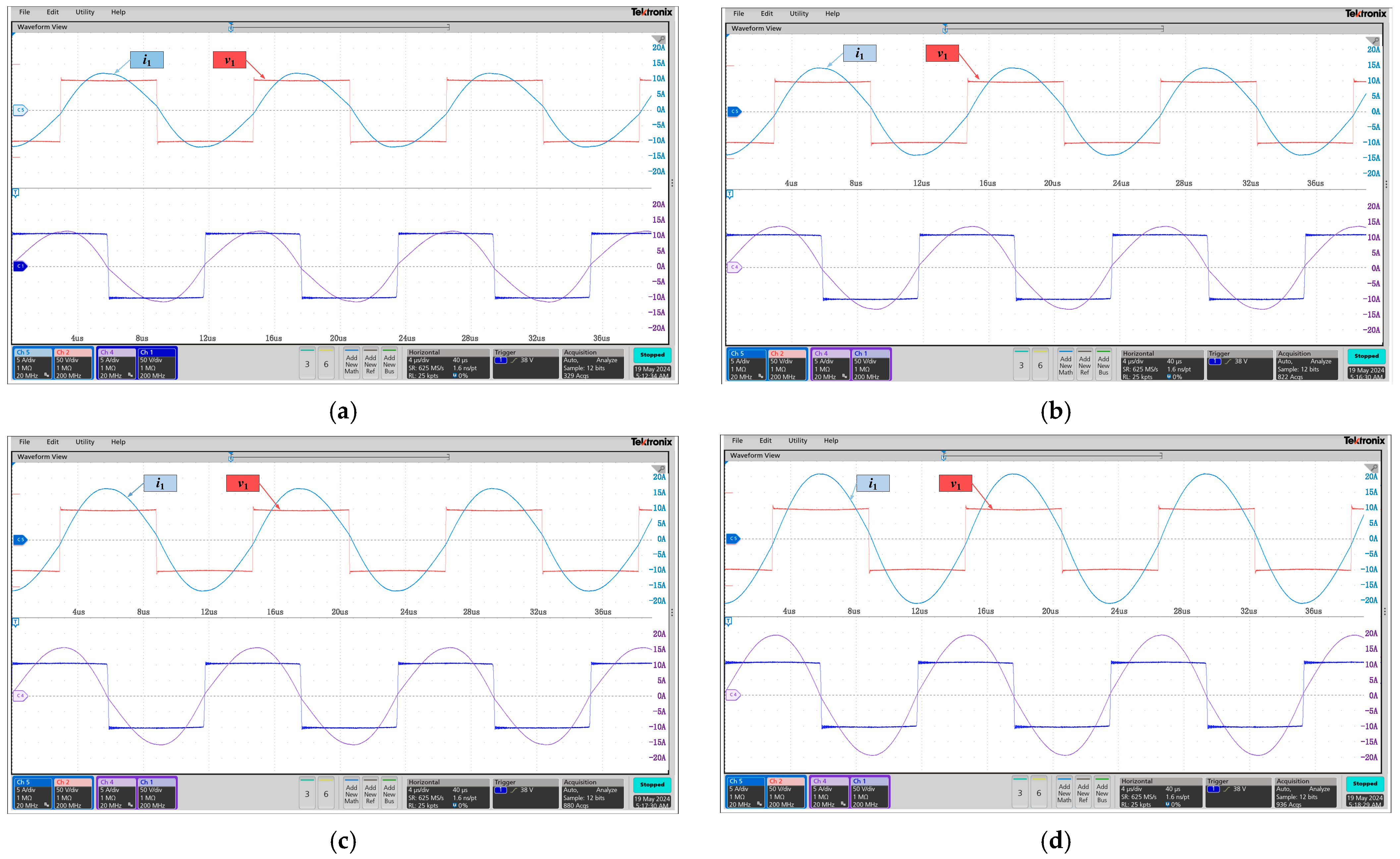
Next, we collect comprehensive data on the primary side currents i₁ and voltages v₁ across various misalignments labeled as X. These data will be utilized to perform a detailed mutual inductance estimation using the proposed method. The collected data for misalignments at X = 0 cm, X = 5 cm, X = 7 cm, and X = 9 cm are displayed in Figure 10a–d.

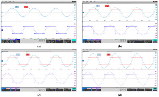
Figure 10. Experiment data at different misalignments. (a) X = 0 cm. (b) X = 5 cm. (c) X = 7 cm. (d) X = 9 cm.

4.2. Data Processing and Mutual Inductance Estimation

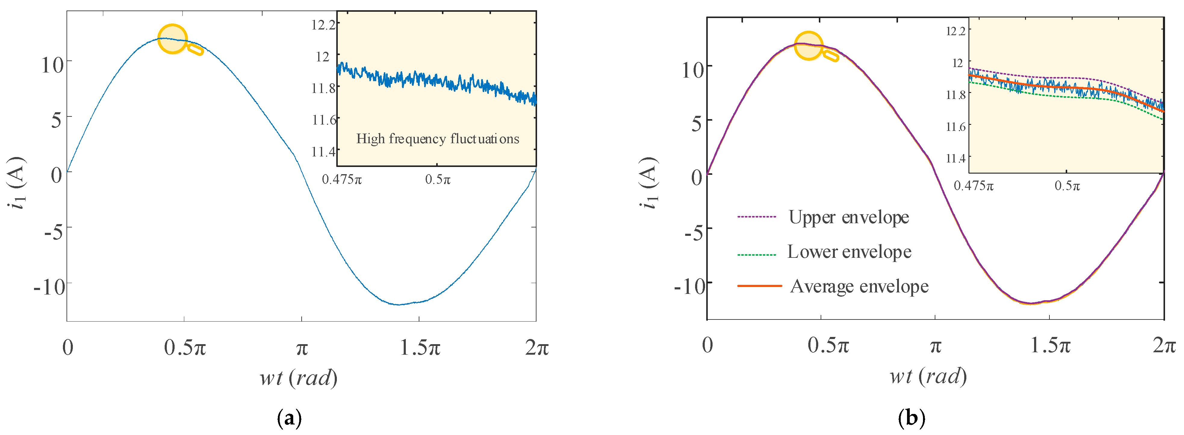
Before the experimental data can be utilized in the proposed method for mutual inductance estimation, it is imperative to perform preprocessing on the raw experimental data. This step is crucial because the experimental data significantly differ from the simulated data, primarily due to the presence of high-frequency noise, as depicted in Figure 11a. Such noise results in the data not being smooth, which could potentially lead to a decrease in the accuracy of the method being proposed. To mitigate this issue, an initial step involves stripping away both the upper and lower envelopes of the data. Following this, the data are further processed by calculating the average of these envelopes, as illustrated in Figure 11b. This averaged envelope data are then used as a refined input for mutual inductance identification.

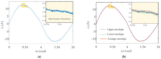
Figure 11. Experimental Data. (a) Raw data. (b) Processed data.

The above processed experimental data under various conditions of misalignment are fed into the proposed method, and the results of mutual inductance estimation are shown in Figure 12. Observations from Figure 12 suggest that, overall, when the misalignment ranges from 0 to 13 cm, corresponding to a coupling coefficient k range from 0.1 to 0.35, the accuracy of mutual inductance identification lies between 92.5% and 96.5%. Notably, at a low coupling coefficient of k = 0.1, the accuracy hits its lowest at 92.5%. As the coupling coefficient increases, there is a noticeable improvement in the predictive accuracy of the proposed method. Specifically, when the coupling coefficient exceeds 0.25, the accuracy of predictions consistently surpasses 95.5%. The proposed mutual inductance estimation method is compared with the existing methods in Table 2, and the proposed method has some attractive features compared with the existing methods. For example, compared with [7], the proposed method can be used when the SS-IPT system operates at the system resonant frequency. Compared to the methods in [8,9], the proposed method can estimate mutual inductance without the information of the output load. Additionally, only a current sensor is required in the proposed method, and, hence, compared with the methods in [11,12], the proposed method has fewer components, leading to reduced cost. Furthermore, compared with the methods in [15,16], the proposed method can estimate mutual inductance without sweeping frequency and without communication, making it suitable for online applications. Finally, the proposed method does not require harmonic extraction, so its results are less affected by the accuracy of harmonic extraction.

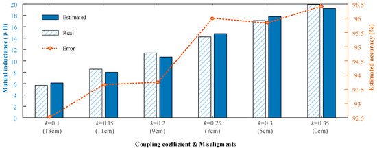
Figure 12. Estimated mutual inductance and the corresponding error under different coupling coefficients with experimental data.

Table 2. Comparison of the proposed mutual inductance estimation method and existing methods.

	Accuracy	Additional Hardware	Commu-nication	Online/Offline	Pregiven Load Information	Time Cost	Disadvantage
[7]	98%	One current sensor	No	Offline	No	/	Cannot work at the system resonant frequency
[8]	93.7–96.2%	One current sensor	No	Online	Load Resistance	/	Only applicable to parallel-tuned secondary power pickup
[9]	99%	One current sensor	No	Online	Load Resistance	4 ms	It is necessary to know the load resistance in advance
[11]	97.8%	One voltage sensor, one additional sandwich coil	No	Online	No	/	Additional design of sandwich coil, replacement of transmitting and receiving coil means redesign, low power density
[12]	97.1%	One switching capacitor	No	Offline	No	50 ms	Additional switches affect efficiency, increase system complexity, and reduce power density
[14]	97%	Two current sensors	Yes	Offline	No	3.6 s	Communication is required, and data at up to 14 frequencies are required to have satisfactory accuracy
[15]	98.5%	One current sensor	No	Offline	No	62 ms	Only applicable to systems with active rectifier and requires frequency sweep
[16]	99%	One current sensor	No	Offline	No	7 ms	Only applicable to systems with active rectifier and requires frequency sweep
[19]	96.6–98%	One current sensor	No	Online	No	2–5 s	Voltage and current of multiple harmonics are required.
This paper	92.5–96.5%	One current sensor	No	Online	No	0.1 s	High sampling rates and high computation are needed.

5. Conclusions

This paper introduces a novel method for estimating mutual inductance in Series-Series inductive power transfer (SS-IPT) systems, using time-domain modeling and nonlinear least squares. Our approach, which relies solely on primary-side information, eliminates the need for additional equipment or complex procedures, simplifying the implementation process. Validated through simulations and experimental data, the method achieves high accuracy rates—over 95.0% in simulations and 92.5% in experiments—demonstrating its effectiveness and potential for enhancing IPT system performance. This streamlined, accurate method offers significant potential for advancing the practical application and efficiency of IPT technologies.

References

- Ma, T.; Jiang, C.Q.; Chen, C.; Wang, Y.; Geng, J.; Tse, C.K. A Low Computational Burden Model Predictive Control for Dynamic Wireless Charging. IEEE Trans. Ind. Electron. 2024, 71, 10402–10413. [Google Scholar] [CrossRef]
- Chen, C.; Jiang, C.; Wang, Y.; Fan, Y.; Luo, B.; Cheng, Y. Compact Curved Coupler With Novel Flexible Nanocrystalline Flake Ribbon Core for Autonomous Underwater Vehicles. IEEE Trans. Power Electron. 2024, 39, 53–57. [Google Scholar] [CrossRef]
- Wang, Y.; Jiang, C.Q.; Chen, C.; Ma, T.; Li, X.; Long, T. Hybrid Nanocrystalline Ribbon Core and Flake Ribbon for High-Power Inductive Power Transfer Applications. IEEE Trans. Power Electron. 2023, 39, 1898–1911. [Google Scholar] [CrossRef]
- Song, K.; Lan, Y.; Zhang, X.; Jiang, J.; Sun, C.; Yang, G.; Yang, F.; Lan, H. A Review on Interoperability of Wireless Charging Systems for Electric Vehicles. Energies 2023, 16, 1653. [Google Scholar] [CrossRef]
- Zou, B.; Huang, Z. Primary-Frequency-Tuning and Secondary-Impedance-Matching IPT Converter With Programmable Constant Power Output and Optimal Efficiency Tracking Against Variation of Coupling Coefficient. IEEE Trans. Power Electron. 2024, 39, 4895–4909. [Google Scholar] [CrossRef]
- Chen, C.; Jiang, C.Q.; Wang, Y.; Ma, T.; Wang, X.; Xiang, J.; Geng, J. High-misalignment Tolerance Inductive Power Transfer System via Slight Frequency Detuning. In Proceedings of the 2023 IEEE Energy Conversion Congress and Exposition (ECCE), Nashville, TN, USA, 29 October–2 November 2023; IEEE: Piscataway, NJ, USA, 2023; pp. 1890–1894. [Google Scholar] [CrossRef]
- Yin, J.; Lin, D.; Parisini, T.; Hui, S.Y. Front-End Monitoring of the Mutual Inductance and Load Resistance in a Series–Series Compensated Wireless Power Transfer System. IEEE Trans. Power Electron. 2016, 31, 7339–7352. [Google Scholar] [CrossRef]
- Su, Y.-G.; Chen, L.; Wu, X.-Y.; Hu, A.P.; Tang, C.-S.; Dai, X. Load and mutual inductance identification from the primary side of inductive power transfer system with parallel-tuned secondary power pickup. IEEE Trans. Power Electron. 2018, 33, 9952–9962. [Google Scholar] [CrossRef]
- Chen, K.; Zhang, Z. Rotating-Coordinate-Based Mutual Inductance Estimation for Drone In-Flight Wireless Charging Systems. IEEE Trans. Power Electron. 2023, 38, 11685–11693. [Google Scholar] [CrossRef]
- Sang, P.; Liu, K.; Gong, B.; Zhang, Y.; Zhang, D.; Huang, C. Mutual Inductance Identification based Constant Voltage Control for LC-L Wireless Power Transmission Systems. In Proceedings of the 2022 25th International Conference on Electrical Machines and Systems (ICEMS), Chiang Mai, Thailand, 29 November–2 December 2022; IEEE: Piscataway, NJ, USA, 2022; pp. 1–5. [Google Scholar]
- Liu, S.; Feng, Y.; Weng, W.; Chen, J.; Wu, J.; He, X. Contactless Measurement of Current and Mutual Inductance in Wireless Power Transfer System Based on Sandwich Structure. IEEE J. Emerg. Sel. Top. Power Electron. 2022, 10, 6345–6357. [Google Scholar] [CrossRef]
- Su, Y.-G.; Zhang, H.-Y.; Wang, Z.-H.; Patrick Hu, A.; Chen, L.; Sun, Y. Steady-State Load Identification Method of Inductive Power Transfer System Based on Switching Capacitors. IEEE Trans. Power Electron. 2015, 30, 6349–6355. [Google Scholar] [CrossRef]
- Zheng, P.; Lei, W.; Liu, F.; Li, R.; Lv, C. Primary Control Strategy of Magnetic Resonant Wireless Power Transfer Based on Steady-State Load Identification Method. In Proceedings of the 2018 IEEE International Power Electronics and Application Conference and Exposition (PEAC), Shenzhen, China, 4–7 November 2018; IEEE: Piscataway, NJ, USA, 2018; pp. 1–5. [Google Scholar] [CrossRef]
- Zhu, G.; Dong, J.; Grazian, F.; Bauer, P. A Parameter Recognition-Based Impedance Tuning Method for SS-Compensated Wireless Power Transfer Systems. IEEE Trans. Power Electron. 2023, 38, 13298–13314. [Google Scholar] [CrossRef]
- Yang, Y.; Tan, S.C.; Hui, S.Y.R. Fast Hardware Approach to Determining Mutual Coupling of Series–Series-Compensated Wireless Power Transfer Systems With Active Rectifiers. IEEE Trans. Power Electron. 2020, 35, 11026–11038. [Google Scholar] [CrossRef]
- Zeng, J.; Chen, S.; Yang, Y.; Hui, S.Y.R. A Primary-Side Method for Ultrafast Determination of Mutual Coupling Coefficient in Milliseconds for Wireless Power Transfer Systems. IEEE Trans. Power Electron. 2022, 37, 15706–15716. [Google Scholar] [CrossRef]
- Liu, J.; Wang, G.; Xu, G.; Peng, J.; Jiang, H. A parameter identification approach with primary-side measurement for DC–DC wireless-power-transfer converters with different resonant tank topologies. IEEE Trans. Transp. Electrif. 2020, 7, 1219–1235. [Google Scholar] [CrossRef]
- Dai, R.; Zhou, W.; Chen, Y.; Zhu, Z.; Mai, R. Pulse density modulation based mutual inductance and load resistance identification method for wireless power transfer system. IEEE Trans. Power Electron. 2022, 37, 9933–9943. [Google Scholar] [CrossRef]
- Dai, R.; Mai, R.; Zhou, W. A Pulse Density Modulation Based Receiver Reactance Identification Method for Wireless Power Transfer System. IEEE Trans. Power Electron. 2022, 37, 11394–11405. [Google Scholar] [CrossRef]
- Wang, K.; Yang, Y.; Zhang, X. Advanced Front-end Monitoring Scheme for Inductive Power Transfer Systems Based on Random Forest Regression. In Proceedings of the 2023 IEEE Applied Power Electronics Conference and Exposition (APEC), Orlando, FL, USA, 19–23 March 2023; IEEE: Piscataway, NJ, USA, 2023; pp. 2901–2907. [Google Scholar] [CrossRef]
- Li, Z.; Li, L. A Digital Twin Based Real-Time Parameter Identification for Mutual Inductance and Load of Wireless Power Transfer Systems. IEEE Access 2023, 11, 55404–55412. [Google Scholar] [CrossRef]
- Chow, J.P.-W.; Chung, H.S.-H.; Cheng, C.-S. Use of Transmitter-Side Electrical Information to Estimate Mutual Inductance and Regulate Receiver-Side Power in Wireless Inductive Link. IEEE Trans. Power Electron. 2016, 31, 6079–6091. [Google Scholar] [CrossRef]
- Chow, J.P.W.; Chung, H.S.H. Use of primary-side information to perform online estimation of the secondary-side information and mutual inductance in wireless inductive link. In Proceedings of the 2015 IEEE Applied Power Electronics Conference and Exposition (APEC), Charlotte, NC, USA, 15–19 March 2015; IEEE: Piscataway, NJ, USA, 2015; pp. 2648–2655. [Google Scholar] [CrossRef]
- Bates, D. Nonlinear Regression Analysis and Its Applications; John Wiley and Sons: Toronto, ON, Canada, 1988; Volume 2, pp. 379–416. [Google Scholar]
- Chavent, G. Nonlinear Least Squares for Inverse Problems: Theoretical Foundations and Step-by-Step Guide for Applications; Springer Science & Business Media: Berlin/Heidelberg, Germany, 2010. [Google Scholar]
Disclaimer/Publisher’s Note: The statements, opinions and data contained in all publications are solely those of the individual author(s) and contributor(s) and not of MDPI and/or the editor(s). MDPI and/or the editor(s) disclaim responsibility for any injury to people or property resulting from any ideas, methods, instructions or products referred to in the content. |
© 2024 by the authors. Licensee MDPI, Basel, Switzerland. This article is an open access article distributed under the terms and conditions of the Creative Commons Attribution (CC BY) license (https://creativecommons.org/licenses/by/4.0/).