Abstract
The introduction of a large number of photovoltaic systems to distribution systems has increased the complexity of the voltage profile. It is thus necessary to manage voltage at a higher system level. For this purpose, the voltage profile of the distribution system can be calculated using state estimation and the voltage can be controlled based on the estimated values. Many methods for estimating voltage profiles using state estimation have been developed. However, the estimation accuracy of voltage profiles required for proper voltage control has not been discussed. If the assumed required estimation accuracy is too high, then more meters than necessary will be installed, unnecessarily increasing costs. Conversely, if the assumed required estimation accuracy is too low, voltage control equipment will not operate properly, and voltage violations may occur. Thus, it is important to determine the required estimation accuracy of voltage profiles for proper voltage control. In this paper, the estimation error of the voltage profile is expressed using a probability density function, and the estimation accuracy of voltage profiles required for proper voltage control is examined. A numerical case study was performed on a distribution network model with 2160 consumers, and revealed the following. To prevent voltage violations, an estimation accuracy of voltage profile that is approximately 10 times lower than that of the estimation accuracy based on current measurement equipment data is sufficient. To minimize the number of tap operations, an estimation accuracy needs to be improved by 70% compared with the estimation accuracy based on current measurement equipment data.
1. Introduction
The number of renewable energy sources has greatly increased in recent years. A large number of photovoltaic (PV) systems have thus been introduced to electrical distribution systems [1]. However, this growth in PV installations has made the voltage profiles along distribution feeders more complicated because the power flow for such installations is bidirectional. Therefore, it is important to estimate voltage profiles based on measurement data to enable proper voltage management in distribution systems with PV installations. Against this background, a number of methods have been proposed for estimating power system voltage profiles using state estimation [2]. A method with additional equality constraints for floating nodes [3], a method that uses Kalman filters [4,5], an estimation method based on asynchronous and synchronous meter data [6], a method that uses historical load data as pseudo-observables [7,8], and a method that uses smart meter data to target low-voltage consumers for estimation [9,10] have been proposed.
Smart meters are being installed for all customers in Japan. The smart meter used in Japan can measure active power consumption at intervals of 30 min [11]. Sensor-embedded sectionalizing switches, called IT switches, have been installed in distribution systems to realize advanced automation control. The authors previously estimated voltage profiles for all nodes, including low-voltage nodes, by performing state estimation on the basis of data from smart meters, IT switches, and distribution substation outfeed points [12].
Several studies [13,14,15] have discussed the relationship between the number and placement of meters and estimation accuracy, which is important for state estimation because voltage profiles are estimated on the basis of measurement data. These studies determined the number and placement of meters required to keep the estimation error of the voltage profile below an arbitrary threshold. However, they did not discuss the estimation accuracy of voltage profiles required for proper voltage control. If the assumed required estimation accuracy is too high, then more meters than necessary will be installed, unnecessarily increasing costs. Conversely, if the assumed required estimation accuracy is too low, voltage control equipment will not operate properly, and voltage violations may occur. Thus, it is important to determine the required estimation accuracy of voltage profiles for proper voltage control.
Methods that combine state estimation and voltage control have also been proposed [16,17]. One study [16] proposed a method for controlling the on-load tap changer (OLTC) after state estimation, and another study [17] proposed a method for Volt/VAR control based on state estimation. However, the estimation accuracy of voltage profiles required for proper voltage control was not discussed.
Numerical simulations with a large amount of input data can be used to clarify the estimation error required for proper voltage control. However, it is difficult to prepare a large amount of input data and verify the relationship between the error and voltage control performance while varying the error magnitude.
In the present study, the voltage profile is estimated on the basis of the state estimation method developed in Ref. [12]. Then, based on the histogram of the estimation error, a probability density function (PDF) is used to model the estimation error of the voltage profile. The relationship between the estimation error magnitude and voltage control is examined by varying the PDF. The estimation accuracy of the voltage profile required for proper voltage control is thus determined. The study of allocation of PV systems with Volt/Var control based on automatic voltage regulators in active distribution networks [18,19], the study of local and remote control of automatic voltage regulators in distribution networks with different variations and uncertainties [20,21], and practical studies [22] are reported. Those studies [18,19,20,21,22] operate voltage control devices based on measurement information from several points. However, the voltage control in the present study assumes that the OLTC is controlled based on voltage profile estimation for all nodes, thus allowing voltage control at higher system levels.
The rest of this paper is organized as follows. Section 2 introduces the voltage control method based on state estimation. Section 3 describes the method used to simulate estimation errors. Section 4 evaluates the estimation accuracy of voltage profiles required for proper voltage control using numerical simulations. Section 5 summarizes the results.
2. Assumed Voltage Control Method
Generally, the voltage of a distribution system is controlled using the OLTC on the basis of data from several measurements. However, this control method is not suitable for distribution systems with PV installations. Therefore, in this paper, the voltage profiles of all nodes in the distribution system are first estimated using state estimation [12]. Then, it is assumed that the OLTC is controlled on the basis of the estimated voltage profile. The OLTC operation is determined from the estimated voltage profile for each operation cycle [17]. The voltage is controlled as follows:
STEP 1: Obtain measurement data from smart meters, IT switches, and feeder points of distribution substations.
STEP 2: Obtain the voltage profile using state estimation based on the measurement data.
STEP 3: Calculate the highest and lowest voltage values ( and , respectively) at each OLTC operation cycle . That is,
where is the voltage estimate obtained using state estimation, and are the highest and lowest voltage values. is the set of nodes in all systems, is the node number, and is time.
STEP 4: Judge whether and violate their respective specified thresholds at each operation cycle . As shown in Figure 1, two thresholds (smax and smin, respectively) are set with a margin of [V] from the upper and lower limits of the allowable voltage range (101 ± 6[V] in Japan). Figure 1 can be explained only by the y-axis (voltage values); there is no x-axis. If and do not violate their respective thresholds, it is determined that the voltage is within the allowed range. Then, the tap operation of the OLTC is not performed at operation cycle t.
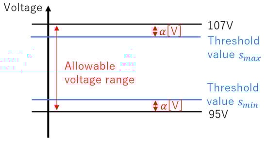
Figure 1.
Specified voltage thresholds.
STEP 5: If drops below its threshold , the OLTC should raise the voltage. Before the OLTC operation, the highest voltage when the OLTC operates is simply estimated using Equation (3).
where is the estimated highest voltage after the OLTC operates, and is the tap width of the OLTC[V].
If exceeds its threshold , the operation of voltage rise by the OLTC can resolve a drop below the threshold , but it newly exceeds the threshold , resulting in hunting. To avoid this situation, the OLTC operation is deactivated if exceeds its threshold . Conversely, if exceeds its threshold , the OLTC should decrease the voltage. However, to avoid hunting, if the lowest voltage after operating the OLTC estimated using Equation (4) drops below threshold , the OLTC operation is deactivated.
where is the estimated lowest voltage after the operation of voltage rise by the OLTC.
A flowchart of the voltage control method is shown in Figure 2.
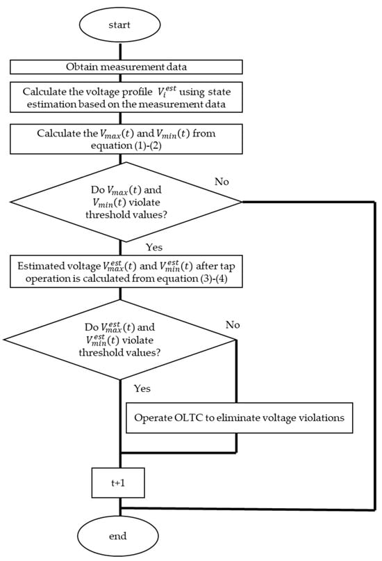
Figure 2.
A flowchart of the voltage control method.
3. Voltage Estimation Model
Numerical simulations with a large amount of input data can be used to clarify the relationship between voltage control and the estimation accuracy of voltage profiles. However, it is difficult to prepare a large amount of input data and conduct numerical simulations while varying the estimation error magnitude. Therefore, in this paper, the inverse transformation method is used to create voltage profile estimation with arbitrary error using the following procedure. First, the target distribution system model, actual measured demand data, and PV data are prepared. Next, the measurement data of smart meters, IT switches, and feeder points of distribution substations installed are created by performing a load flow calculation based on the prepared data. Then, the voltage profile of the distribution system is estimated from the created measurement data using state estimation, since the distribution system operator only obtains the measured data. The voltage profile of the distribution system is estimated using constrained state estimation [3] with the following equation.
where is a vector of the measurement data, is a vector whose elements represent the values corresponding to the measurements in calculated from the state values , is a vector whose elements represent the active and reactive power injections at the floating nodes, and is a diagonal weighting matrix. and can be obtained using Kirchhoff’s voltage and current laws. and are the voltage [V] and phase angle [rad] at the i-th node, respectively, and L is the total number of nodes in the distribution system.
A histogram is created from the estimation error in the voltage profile for each node. A PDF is fitted to the histogram using the maximum likelihood estimation (MLE) method. A general continuous function is used for the PDF. The maximum and minimum PDF values are, respectively, determined by the maximum and minimum estimation errors.
The simulated estimation error is then obtained from the uniform random number and the inverse cumulative distribution function corresponding to the PDF using Equation (8). The simulated voltage profile estimation is expressed in Equation (9).
where is the estimation error of the voltage profile, is the inverse cumulative distribution function of the PDF, is a uniform random number, is the true value of the voltage profile, k is a variable that changes the error magnitude, and the subscripts and , respectively, denote the node number and time.
It is possible that the estimation accuracy of the voltage profile may vary depending on the uncertainty of the measurements. In this paper, it is possible to vary the accuracy of the voltage profile estimation by varying the value of k in Equation (9). By changing the value of k, the effect of the uncertainty of the measurement equipment on the estimation accuracy of the voltage profile can be taken into account. The relationship between the estimation error magnitude and voltage control is examined by varying k in Equation (9).
4. Numerical Case Studies
4.1. Simulation Conditions
4.1.1. System Model
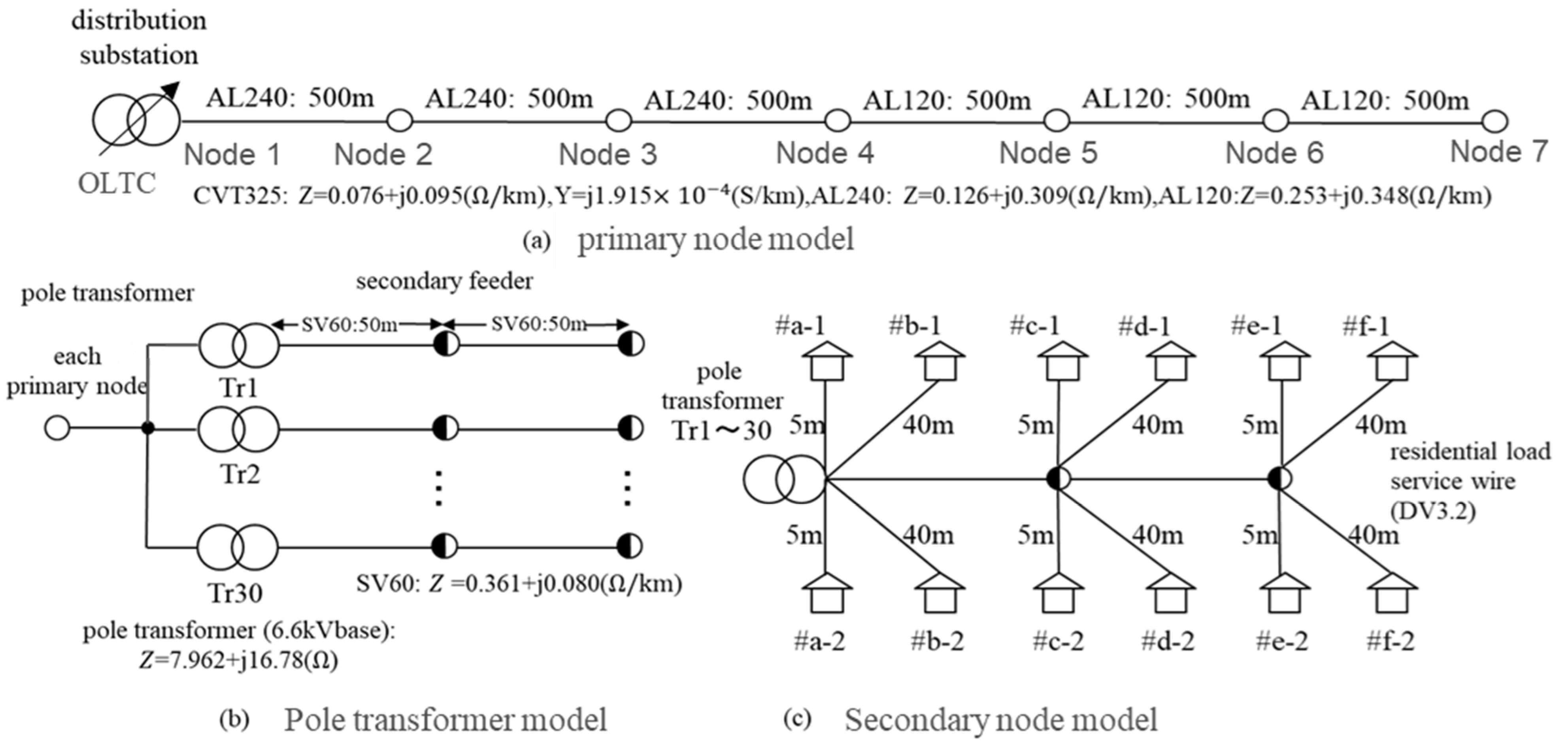
The relationship between the estimation error of the voltage profile and the control performance was examined using the distribution system model shown in Figure 3 [23]. The system model has six primary (high-voltage) nodes. Each high-voltage node serves 30 pole transformers, each of which is connected to 12 customers through secondary feeders. Thus, the system has a total of 2160 customers. A PV system is installed for each consumer.

Figure 3.
Distribution system model; (a) primary node model, (b) pole transformer model, and (c) secondary node model.
4.1.2. Demand and PV Data
The demand (active and reactive powers) and PV output data were prepared on the basis of actual measurement data for a demonstration project of the New Energy and Industrial Technology Development Organization (NEDO) in Ota City, Gunma Prefecture, Japan (called Ota data, hereafter). In the NEDO demonstration project [24], PV was installed in 553 households, and the one-second values of active and reactive power for each customer’s load and PV output were measured for one year. The Ota data also include reactive power data, but the reactive power may be due to the leading power factor operation of the power conditioning system (PCS) as a countermeasure against voltage increase. The model used in the estimation (Figure 3) is not the distribution system model of Ota City. If the reactive power data contained in the Ota data are used directly, there is a possibility that the leading power factor operation data of the PCS will be assigned even though the receiving voltage is within the correct voltage range. On the other hand, data in which the PCS is operating with a power factor of 1, even though the receiving voltage is outside the proper voltage range, may be assigned, which is not appropriate. Therefore, the reactive power output of the PCS was generated using the following procedure.
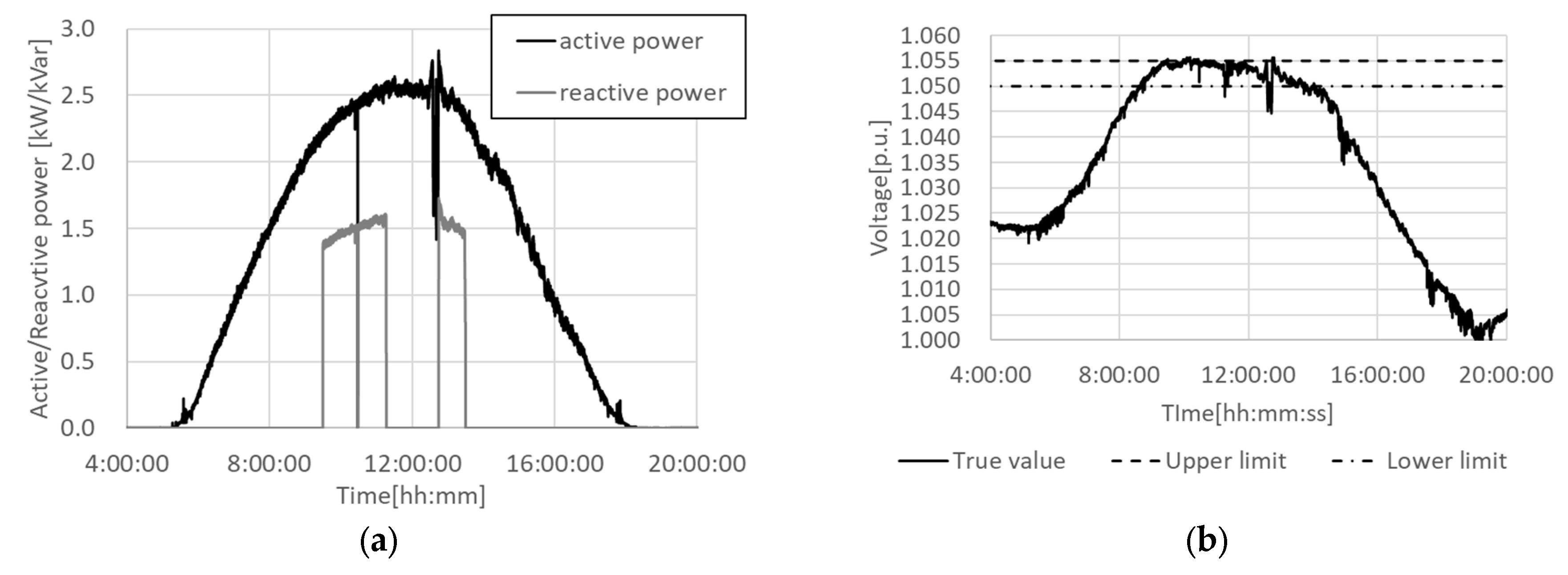
First, under the assumption of zero reactive power injection by the PCS, a load flow calculation was carried out in chronological order for the Ota data. If the terminal voltage of the PCS continuously exceeded the upper threshold (105.5 V) for 10 s, the operating power factor of the PCS was adjusted toward the leading phase until the terminal voltage fell below the lower threshold (105.0 V). If the receiving voltage was less than the lower threshold, but the PCS still injected leading reactive power, unnecessary reactive power injection was gradually reduced until the terminal voltage exceeded the lower threshold. As an example, the active and reactive power outputs of the PCS at a customer are shown in Figure 4a and the terminal voltage is shown in Figure 4b. The values created using the above procedure were used as the truth data.
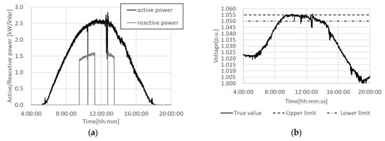
Figure 4.
True value data for (a) active and reactive power and (b) voltage (standard voltage is 100 V).
4.1.3. Measurement Data
The measurement data from smart meters, IT switches, and distribution substation feed points are available in Japan. Those measurement data were created by performing a load flow calculation based on the truth data (Ota data). It was assumed that the measurement data could be time-synchronized. The specifics of each type of measurement data are shown below:
- The 30 min average active power consumption for each customer, measured by a smart meter. It was assumed that the data collection interval of the smart meter was 30 min with a 1 h delay (i.e., the average active power consumption from 8:30 to 9:00 was available at 10:10);
- Instantaneous values of voltage magnitude and passing active and reactive power flows at IT switches. The root mean square (RMS) is used for the instantaneous value of magnitude. The assumed sampling time was 1 min;
- Instantaneous values of voltage magnitude and sending active and reactive power flows at the distribution substation. RMS is used for the instantaneous value of magnitude. The assumed sampling time was 1 min.
4.1.4. Specifications of OLTC
The OLTC taps can be changed in 30 V (high-voltage equivalent; low-voltage equivalent: 0.477 V) increments within the range of 6060–6660 V. The initial position of the tap was set at 6360 V (low-voltage equivalent: 101.2 V), which was the center of the available tap positions. In STEP 5 of the voltage control, it is judged twice whether the voltage estimation violates the thresholds. The first judgment is made whether the voltage profile estimation before the operation of the OLTC calculated by Equations (1) and (2) violates the threshold value. A simulation was performed by varying the margin of [V], which determines the thresholds at the first judgment. The second judgment is made whether the voltage estimation after the operation of the OLTC calculated by Equations (3) and (4) violates the thresholds. The thresholds at second judgment were fixed at a value with a margin of 0.5 V from the upper and lower voltage limits in the simulation. The OLTC is assumed to be controlled every 10 min based on the estimated voltage profile at each operation cycle.
4.1.5. Creation of Histograms and PDFs
To create the histograms, voltage profiles are estimated for a 1 min period using the April Ota data for the distribution system shown in Figure 3. Then, a histogram (and its corresponding PDF) is created from the estimation error of the voltage profile for each node. The maximum and minimum values of the PDF are determined by the maximum and minimum errors of each node, respectively. To create a PDF with accurate shapes, it is essential to construct histograms based on a substantial number of samples of estimation errors. Although the control cycle of the OLTC was 10 min, the estimation was made in 1 min cycles to ensure an adequate number of samples for the estimation error.
4.2. Simulation Results
4.2.1. Histogram and PDF Fitting Using MLE Method
Figure 5 shows a histogram of the estimation error of the voltage profile for Ota data. It can be seen that the shape of the histogram is close to that of the t-distribution. Therefore, in this paper, the t-distribution given in Equation (10) is used as the PDF. The shape parameters (μ, σ, and ν) in Equation (10) are obtained by MLE.
where PDF is the probability density function following a t-distribution, is random numbers following a uniform distribution, Γ is the gamma function, and μ, σ, and ν are shape parameters.
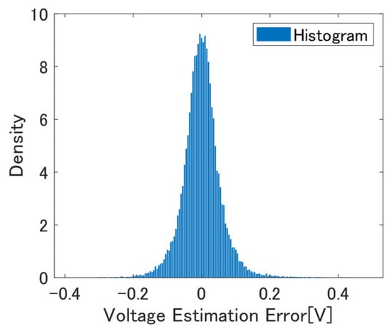
Figure 5.
Histogram of voltage estimation error at end node.
Figure 6 shows the results of fitting the PDF to the histogram using the MLE method. Note that the histogram shows the results for the end node as an example. The histograms are normalized to have an area of 1 to conform to the PDF. As shown in Figure 6, the PDF fits the histogram well by using t-distribution.
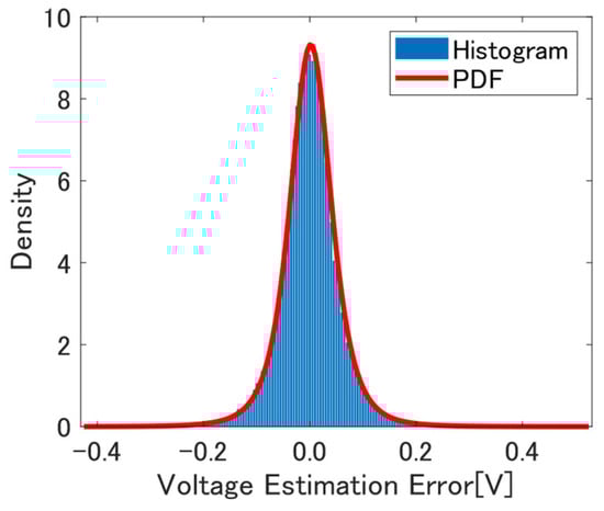
Figure 6.
Histogram of voltage estimation error at end node and PDF fitting result.
4.2.2. OLTC Malfunction and Non-Operation
To discuss the relationship between the estimation error and control, we define and as the time series data of the tap position when the OLTC is controlled on the basis of the voltage profile of the true value. and , respectively, represent the time series data of the tap position before and after the STEP 5 judgment of the voltage control. The time series data of the tap position when the OLTC is controlled on the basis of the voltage profile estimated using Equation (9) are denoted as . is created as follows. In each OLTC control cycle, the tap position before the STEP 5 judgment is , and that after the STEP 5 judgment is , which is determined from the estimated voltage and . If and are equal, the voltage control is operating normally. However, if and are different, the operation of the OLTC is judged to be malfunctioning or non-operational. In the operating cycle t of the OLTC, it is considered non-operational if the is operating but not operating at . It is considered a malfunction if is operating while is not operating. The voltage control is evaluated in terms of the number of malfunctions and non-operations.
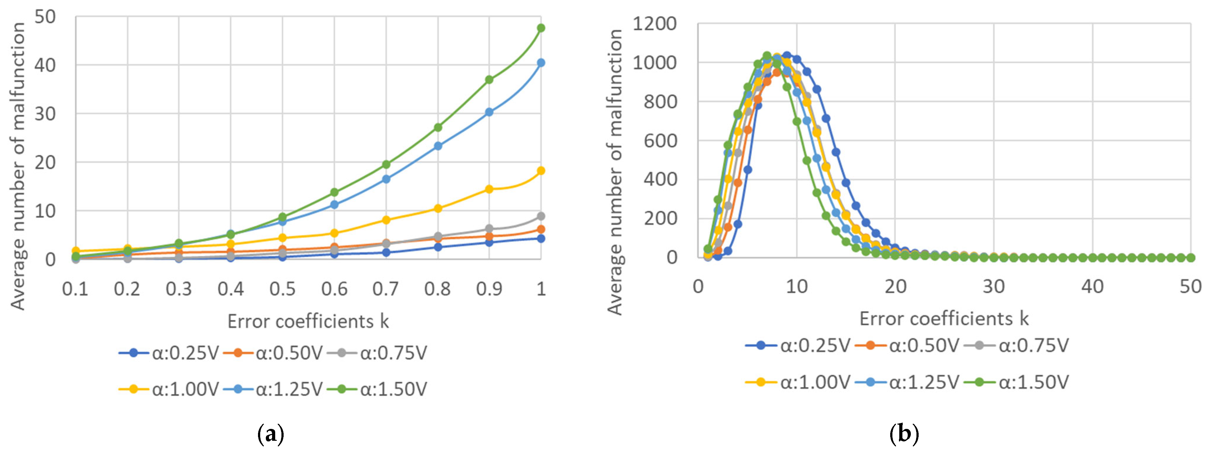
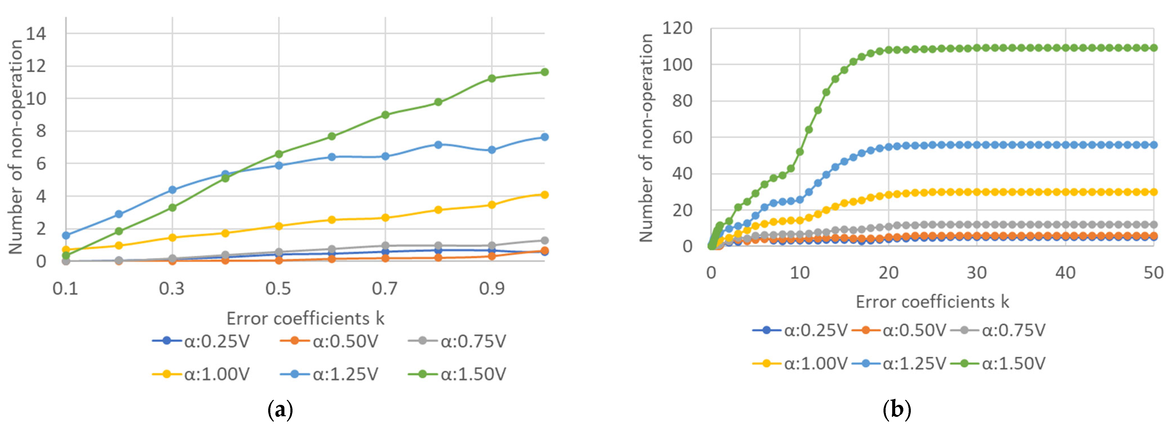
The simulation was conducted 100 times for the month of April. Figure 7 and Figure 8 show the results of the average number of malfunctions and non-operations for k in the ranges of 0.1–1.0 and 1.0–50.0. The margin for setting the threshold was varied in the range of 0.25~1.5 V. Figure 7b shows that the average number of malfunctions initially increases and then decreases with increasing k. As the estimation error of the voltage profile increases, the voltage profile estimation becomes more likely to violate the threshold value (first judgment). Thus, the number of malfunctions increases. In STEP 5 of the voltage control, if the estimated voltage profile after the OLTC tap is operated violates the threshold value (second judgment), the OLTC tap is not operated. With a further increase in k, the estimated voltage profile in STEP 5 of the voltage control violates the threshold value (second judgment) and the OLTC tap operation is suppressed. This leads to a decrease in the number of malfunctions. As shown in Figure 8b, the number of non-operations initially increases as k increases and then remains constant. This is because the tap did not operate because of the suppression of the tap operation in STEP 5.
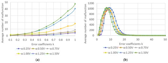
Figure 7.
Average number of malfunctions versus error coefficient k for (a) k = 0.1–1.0 and (b) k = 1.0–50.0.
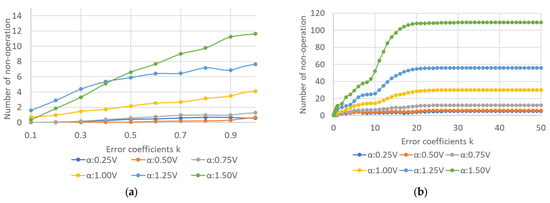
Figure 8.
Average number of non-operations versus error coefficient k for (a) k = 0.1–1.0 and (b) k = 1.0–50.0.
As shown in Figure 7a and Figure 8a, the number of malfunctions and non-operations decreases as the value of k decreases in the range of 0.1–1.0. This indicates that approaches as the estimation error of the voltage profile becomes smaller. However, there are cases where the number of malfunctions is not zero, even for k = 0.1, which is equivalent to 10 times the accuracy of estimating voltage profiles using the present measurement equipment. When the true value of the voltage profile and the threshold value are close, a small estimation error will result in a malfunction or non-operation. Therefore, regardless of the improvement in the accuracy of the voltage profile estimation, it is difficult to reduce the number of malfunctions and non-operations to zero. Thus, the number of malfunctions and non-operations cannot be used to discuss the accuracy of the voltage profile estimation required for proper voltage control.
4.2.3. Number of Tap Operations and Voltage Violations
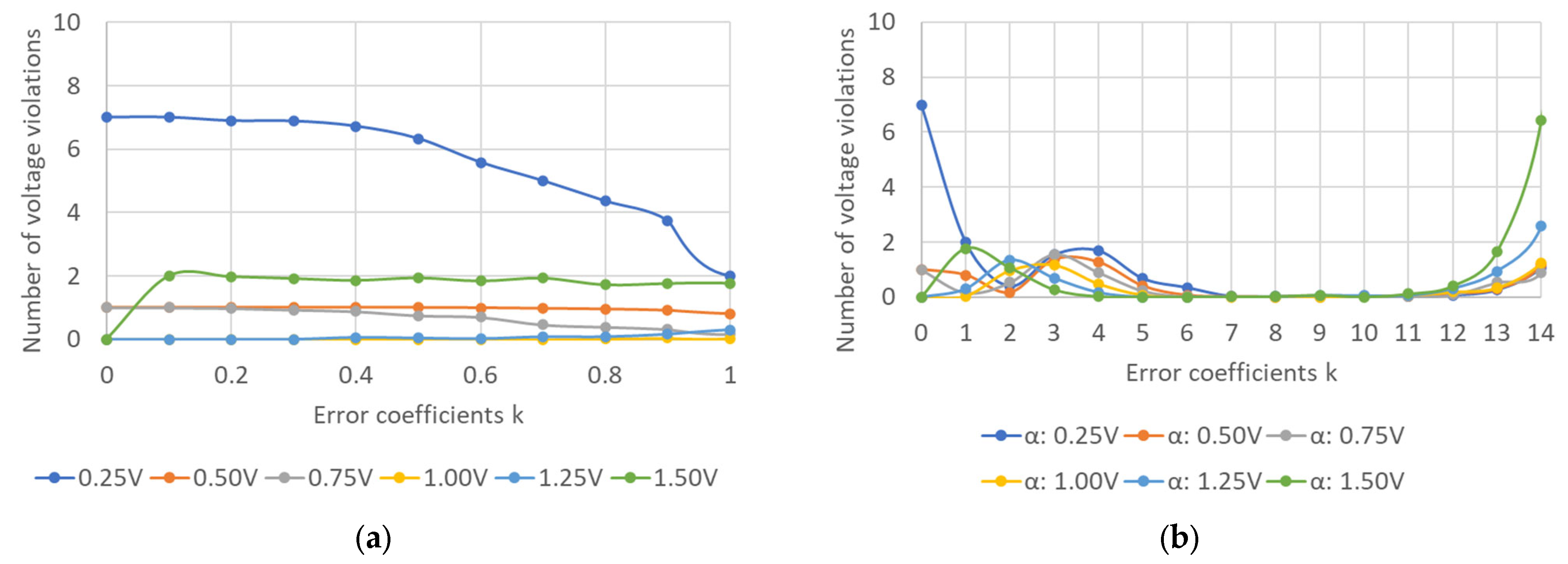
In the previous section, simulations were performed under the assumption that the tap position based on voltage estimation before the judgment in STEP 5 is equal to . In this section, the tap positions determined from the voltage profile estimation are carried over to the next time step. In other words, if the tap positions before and after the judgment in STEP 5 are newly defined as and , then . Figure 9, Figure 10 and Figure 11 show the results of 100 simulations conducted for the month of April. The margin for setting the threshold was varied in the range of 0.25~1.5 V. Each figure shows the average number of voltage violations, the average number of tap operations, and the average number of suppressed tap operations. The results for k = 0 represent those obtained with the OLTC controlled on the basis of the true value of the voltage profile . Figure 9a shows that even when the OLTC is controlled on the basis of the true value of the voltage profile, a voltage violation still occurs when the margin width is less than 0.75 V. This is because the voltage value fluctuated above the margin width within 10 min of an OLTC control cycle. In addition, there are cases where the number of voltage violations decreases as k increases. This is because as the estimation error increases, the voltage threshold is more likely to be violated and the tap operation is more likely to occur. This tap operation reduced the number of voltage violations. Figure 9b shows that the number of voltage violations initially decreased and then increased after k = 10. This result indicates that when the purpose of voltage control is to prevent voltage violations, an estimation accuracy that is 10 times lower than the current estimation accuracy is sufficient. In other words, the number of measurement devices or their performance can be reduced compared with the presently assumed values.
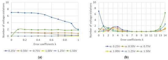
Figure 9.
Average number of voltage violations versus error coefficient k for (a) k = 0.1–1.0 and (b) k = 1.0–14.0.
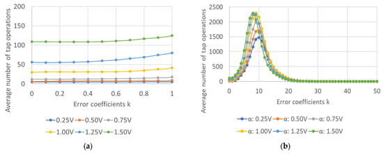
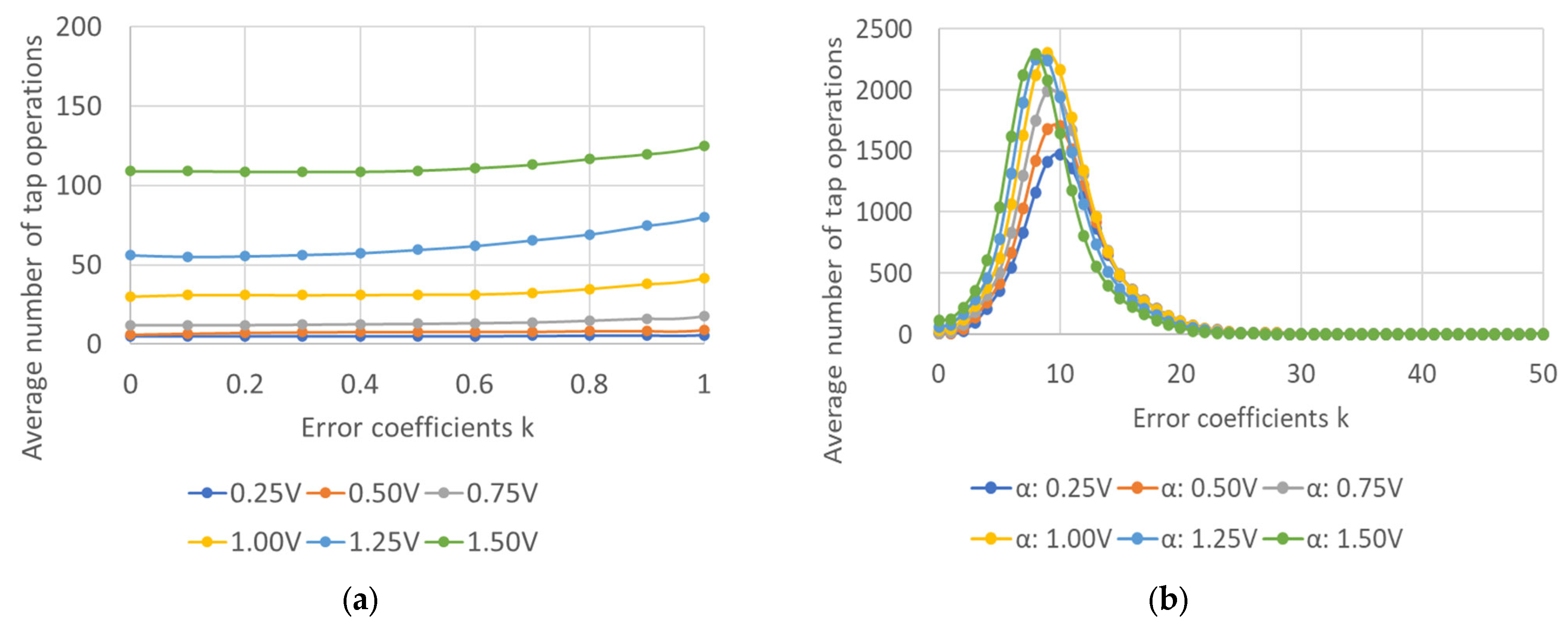
Figure 10.
Number of tap operations versus error coefficient k for (a) k = 0.1–1.0 and (b) k = 1.0–50.0.

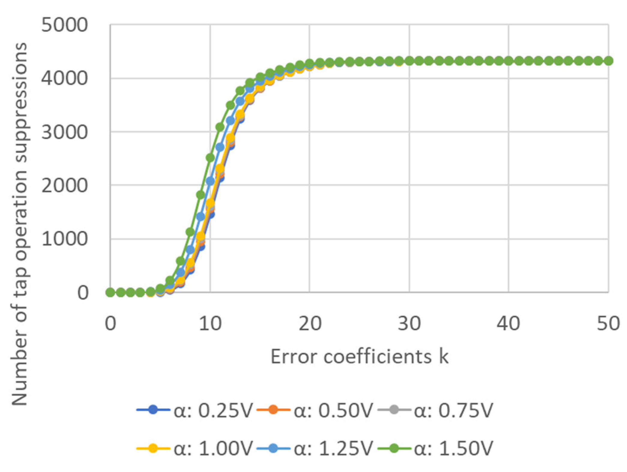
Figure 11.
Average number of tap operation suppressions versus error coefficient k for k = 1.0–50.0.
Figure 10b shows that the number of tap operations initially increases and then decreases as k increases. As explained in the previous section, STEP 5 of voltage control has two judgments as to whether the voltage estimation violates the thresholds. The number of times that the voltage estimation violates thresholds in the first judgment increases as k increases. Therefore, the number of tap operations is initially increasing. As k increases further, the number of times the voltage estimation violates thresholds in the second judgment increases, and thus the tap operation is suppressed to prevent hunting. Figure 11 shows that the number of tap operation suppressions increases, and thus the number of tap operations decreases as k increases. Figure 10a shows that the increase in the number of tap operations compared with that when the true value of the voltage profile is known is limited to one in all cases up to k = 0.3. Frequent tapping wears out the OLTC and reduces its service life. Therefore, fewer tapping operations are desirable. The number of tap operations is minimized when the true value of the voltage profile is known. For the number of tap operations to be the same as that when the true value is known, it is necessary to improve the current estimation accuracy by 70%. To improve the accuracy of voltage profile estimation, the number of measurement devices or their performance must be increased compared with the presently assumed values because the estimated voltage profile depends on the measurement information. While this study was conducted using a simple system model, it is expected that the estimated error values for the voltage profiles and PDF shape would differ when simulated using other models. However, the proposed method is applicable to actual complex system models. Simulation with other system models is a subject for future work.
5. Conclusions
The control of an OLTC on the basis of voltage profile estimation was studied for a large number of PV systems installed in an electrical distribution system. The estimation accuracy of the voltage profile required to properly control the voltage for OLTC control was determined. When the purpose of voltage control is to prevent voltage violations, an estimation accuracy that is approximately 10 times lower than that of the estimation of voltage profiles based on current measurement equipment is sufficient. If the number of tap operations is to be reduced, the accuracy needs to be improved by 70% compared with the current accuracy. Future work will include additional simulations on various distribution systems. The accuracy of voltage profile estimation required to properly control voltage using various controllers will also be examined.
Author Contributions
Conceptualization, R.A., R.H., H.K., S.S. and T.K.; methodology, R.A., R.H., H.K., S.S. and T.K.; software, R.A.; validation, R.A., R.H., H.K., S.S. and T.K.; formal analysis, R.A., R.H., H.K., S.S. and T.K.; investigation, R.A.; resources, R.A., R.H., H.K., S.S. and T.K.; data curation, R.A.; writing—original draft preparation, R.A. and R.H.; writing—review and editing, R.A. and R.H.; visualization, R.A.; supervision, R.H. and H.K; project administration, R.A., R.H. and H.K.; funding acquisition: R.A., R.H. and H.K. All authors have read and agreed to the published version of the manuscript.
Funding
This research was funded by JST, the establishment of university fellowships towards the creation of science technology innovation, grant number JPMJFS2101. The APC was funded by JPMJFS2101.
Data Availability Statement
Data are contained within the article.
Acknowledgments
We thank Adam Przywecki for editing a draft of this manuscript.
Conflicts of Interest
Authors Shuhei Sugimura and Toshiharu Kurihara were employed by the company Meidensha Corp. The remaining authors declare that the research was conducted in the absence of any commercial or financial relationships that could be construed as a potential conflict of interest.
References
- Hemetsberger, W.; Schmela, M.; Cruz-Capellan, T. Global Market Outlook For Solar Power 2023–2027; SolarPower Europe: Brussels, Belgium, 2023. [Google Scholar]
- Zhao, J.; Gomez-Exposito, A.; Netto, M.; Mili, L.; Abur, A.; Terzija, V.; Kamwa, I.; Pal, B.; Singh, A.K.; Qi, J.; et al. Power system dynamic state estimation: Motivations, definitions, methodologies, and future work. IEEE Trans. Power Syst. 2019, 34, 3188–3198. [Google Scholar] [CrossRef]
- Wu, F.F.; Liu, W.H.; Lun, S.M. Observability analysis and bad data processing for state estimation with equality constraints. IEEE Trans. Power Syst. 1988, 3, 541–548. [Google Scholar] [CrossRef]
- Wang, K.; Liu, M.; He, W.; Zuo, C.; Wang, F. Koopman Kalman Particle Filter for Dynamic State Estimation of Distribution System. IEEE Access 2022, 10, 111688–111703. [Google Scholar] [CrossRef]
- Carquex, C.; Rosenberg, C.; Bhattacharya, K. State Estimation in Power Distribution Systems Based on Ensemble Kalman Filtering. IEEE Trans. Power Syst. 2018, 33, 6600–6610. [Google Scholar] [CrossRef]
- Muscas, C.; Pau, M.; Pegoraro, P.A.; Sulis, S. Uncertainty of Voltage Profile in PMU-Based Distribution System State Estimation. IEEE Trans. Instrum. Meas. 2016, 65, 988–998. [Google Scholar] [CrossRef]
- Baran, M.; Kelley, A. State Estimation for Real-time Monitoring of Distribution Systems. IEEE Trans. Power Syst. 1994, 9, 1601–1609. [Google Scholar] [CrossRef] [PubMed]
- Lu, C.N.; Teng, J.H.; Liu, W.H. Distribution System State Estimation. IEEE Trans Power Syst. 1995, 10, 229–240. [Google Scholar] [CrossRef]
- Huang, M.; Wei, Z.; Pau, M.; Ponci, F.; Sun, G. Interval State Estimation for Low-Voltage Distribution Systems Based on Smart Meter Data. IEEE Trans Instrum. Meas. 2019, 68, 3090–3099. [Google Scholar] [CrossRef]
- Alzate, E.B.; Bueno-Lopez, M.; Xie, J.; Strunz, K. Distribution System State Estimation to Support Coordinated Voltage-Control Strategies by Using Smart Meters. IEEE Trans. Power Syst. 2019, 34, 5198–5207. [Google Scholar] [CrossRef]
- Ministry of Economy, Trade and Industry. Next Generation Smart Meter System Study Group Summary; Ministry of Economy, Trade and Industry: Tokyo, Japan, 2022. (In Japanese)
- Akasaka, R.; Hara, R.; Kita, H.; Tanabe, T.; Sugimura, S. Voltage Profile Estimation using State Estimation in a Distribution Network. IEEJ Trans. Power Energy 2021, 141, 440–447. (In Japanese) [Google Scholar] [CrossRef]
- Singh, R.; Pal, B.C.; Jabr, R.A. Measurement Placement in Distribution System State Estimation. IEEE Trans. Power Syst. 2009, 24, 668–675. [Google Scholar] [CrossRef]
- Pegoraro, P.A.; Sulis, S. Robustness-Oriented Meter Placement for Distribution System State Estimation in Presence of Network Parameter Uncertainty. IEEE Trans. Instrum. Meas. 2013, 62, 954–962. [Google Scholar] [CrossRef]
- Liu, J.; Ponci, F.; Monti, A.; Muscas, C.; Pegoraro, P.A.; Sulis, S. Optimal Meter Placement for Robust Measurement Systems in Active Distribution Grids. IEEE Trans. Instrum. Meas. 2014, 63, 1096–1105. [Google Scholar] [CrossRef]
- Hanai, Y.; Hayashi, Y.; Matsuki, J.; Kurihara, M. Proposal and Experimental Verification of Distribution Voltage Estimation and Control Method using Measured Data from IT Switches. IEEJ Trans. Power Energy 2010, 130, 859–869. (In Japanese) [Google Scholar] [CrossRef]
- Deshmukh, S.; Natarajan, B.; Pahwa, A. State Estimation and Voltage/VAR Control in Distribution Network with Intermittent Measurements. IEEE Trans. Smart Grid 2014, 5, 200–209. [Google Scholar] [CrossRef]
- Mendoza, J.E.; Morales, D.A.; Lopez, R.A.; Lopez, E.A.; Vannier, J.C.; Coello, C.A.C. Multiobjective Location of Automatic Voltage Regulators in a Radial Distribution Network Using a Micro Genetic Algorithm. IEEE Trans. Power Syst. 2007, 22, 404–412. [Google Scholar] [CrossRef]
- Safigianni, A.S.; Salis, G.J. Optimum voltage regulator placement in a radial power distribution network. IEEE Trans. Power Syst. 2000, 15, 879–886. [Google Scholar] [CrossRef]
- Elkhatib, M.E.; El-Shatshat, R.; Salama, M.M.A. Novel Coordinated Voltage Control for Smart Distribution Networks with DG. IEEE Trans. Smart Grid 2011, 2, 598–605. [Google Scholar] [CrossRef]
- Zhang, L.; Liu, Y.; Liang, D.; Kou, P.; Wang, Y.; Gao, Y.; Li, D.; Liu, H. Local and Remote Cooperative Control of Hybrid Distribution Transformers Integrating Photovoltaics in Active Distribution Networks. IEEE Trans. Sustain. Energy 2022, 13, 2012–2026. [Google Scholar] [CrossRef]
- Tanabe, T.; Nakashima, H.; Hayashi, T. Initiatives for the Development of Autonomous Decentralized Voltage Control Technology with Distribution Systems—Next Generation Transmission and Distribution System Optimal Control Technology Demonstration Project—MEIDEN Time Tone. Volume 336, No. 3, pp. 38–45, 2012. Available online: https://www.meidensha.co.jp/rd/rd_01/rd_01_02/rd_01_02_14/rd_01_02_14_01/pdf/article-201203-0038.pdf (accessed on 17 December 2023). (In Japanese).
- Electric Technology Research Association. Harmonic Disturbance Prevention Measures in Distribution Systems; Electric Technology Research 37; Electric Technology Research Association: Tokyo, Japan, 1981. (In Japanese) [Google Scholar]
- Technology Development Organization. Demonstration Study of Concentrated Interconnected Photovoltaic Generation System. Available online: https://www.nedo.go.jp/activities/ZZ_00229.html (accessed on 17 December 2023). (In Japanese).


Disclaimer/Publisher’s Note: The statements, opinions and data contained in all publications are solely those of the individual author(s) and contributor(s) and not of MDPI and/or the editor(s). MDPI and/or the editor(s) disclaim responsibility for any injury to people or property resulting from any ideas, methods, instructions or products referred to in the content. |
© 2023 by the authors. Licensee MDPI, Basel, Switzerland. This article is an open access article distributed under the terms and conditions of the Creative Commons Attribution (CC BY) license (https://creativecommons.org/licenses/by/4.0/).