Analysis of Flexibility Potential of a Cold Warehouse with Different Refrigeration Compressors

Abstract

The research into new approaches to shift from fossil fuels to renewable energy sources (RES) has surged as environmental issues are on the rise, and fossil fuel sources are becoming scarce. The flexibility potential of cold supply systems has been discussed widely in the literature, firstly due to their high share of electricity consumption worldwide and secondly because of their potential to store thermal energy in the form of cold energy. However, finding a clear definition of flexibility and a concise approach for its quantification is still under progress. In this work, a comprehensive definition of the flexibility of energy systems and a novel methodology for its quantification are introduced. The methodology was applied on a cold warehouse with real data regarding its cold energy demand. The cold warehouse was first modeled via oemof, which is a modular open source framework developed in Python 3.8 using a mixed integer linear programming (MILP) optimization approach. The operation optimization of the cold warehouse was conducted for three goals, namely “minimization of electricity costs”, “minimization of CO₂ emissions”, and “minimization of maximum used electric power (peak load minimization)”. Additionally, the effect of using different types of refrigeration compressors on the optimized operation of the cold warehouse was investigated. The results suggest that a cold warehouse possesses a high level of flexibility potential, which can be taken advantage of to reduce the electricity cost by up to 50%, the CO₂ emissions between 25% to 30%, and the maximum used electric power by 50%. Different compressor types produced very similar results, although their flexibility level may vary.

1. Introduction

Fossil fuels are still the main source of energy used to meet the electricity demand in the world, despite their negative impacts on the environment [1]. Moreover, many traditional end-energy users have been electrified [2], which has risen the demand for electricity drastically. In addition, the energy costs, including electricity costs, have increased drastically recently due to the Ukraine war [3] and also continuously in the last decade [4], which has put many households and industries under pressure. Renewable energy sources (RES) were introduced as an eco-friendly solution to the environmental issues caused by fossil fuels and the growing demand in the electricity market [1,5]. However, the integration of RES into the electricity grids, due to their unpredictable and volatile nature, comes along with a number of challenges, such as substantial load changes, instability in energy supply, shortage of transmission grid capacity, generation inadequacy with grids reaching their limits, higher peak loads, and sophisticated control dilemmas [2,5,6,7]. Consequently, a pressing need has arisen to find immediate solutions to such consequent challenges.

Demand-side management (DSM), with the potential to act as a standing reserve, is one plausible solution to the uncertainty caused by intermittent RES and to maintain the balance in the energy market between demand and supply [8,9,10,11]. DSM can also be implemented to reduce electricity costs by avoiding expensive peaks and purchasing energy in periods of low prices [4,9] in market-driven regions. However, DSM measures are closely tied to the level of flexibility of an energy system [12]. Therefore, it is of crucial significance to profoundly discuss different aspects of flexibility in energy systems and the ways it can be added to them. Thermal energy storage (TES), as one of the main tools that adds flexibility to an energy system [13], contributes to DSM measures and allows for the integration of RES into the electricity production mix and also electrical load shift from peak periods to off-peak periods [14]. Refrigeration systems are one of the main areas in which TES finds vast application. One advantage of refrigeration systems over other energy systems is their inherent thermal storage capacity [15]. This means that the cold thermal energy can be stored in such systems simply by lowering the temperature of the refrigerated goods without requiring external energy storage. For instance, it is possible to use the stored refrigerated goods in a cold warehouse, as cold thermal storage decreases the complexity and costs of implementing DSM measures [16]. Additionally, external cold energy storage can be installed [15]. Moreover, the refrigeration sector is one of the largest energy consumers, with 15–17% of the worldwide electricity consumption [17,18], which makes it a perfect target for energy management analysis. Industrial refrigeration systems, including cold warehouses, rank among the heaviest electricity consumers [16], which is why this paper placed its focus on introducing a definition and a novel approach to quantify and evaluate the flexibility of cold supply systems with the example of a cold warehouse.

This paper contributes to the on-going research into demand-side management as a strategy to combat the existing dilemmas of the energy market by studying the flexibility potential of cold supply systems. The aim of this work was to firstly present a comprehensive definition of the flexibility of energy systems and secondly to provide a novel methodology for its quantification. The developed method was implemented on a cold warehouse with four different types of refrigeration compressors as a case study in pursuit of economic, ecological, and technical goals. Section 2 provides an in-depth literature review of the definition of flexibility for energy systems, followed by a comprehensive definition of flexibility of energy systems, which has been developed in this work. Afterwards, the existing methods to quantifying the flexibility of energy systems are profoundly discussed in Section 3, followed by a novel approach to the quantification of flexibility of energy systems developed in this work. In Section 4, it is explained how a cold warehouse is modeled in this work. The results are presented and discussed in Section 5. The paper ends with a conclusion in Section 6.

2. Definition of Flexibility

The flexibility of energy systems has been addressed so differently in the literature that it can be claimed that there is no consensus over its definition [19,20] and aspects [2]. In fact, a wide range of concepts, from very general to very specific, has been used to define and quantify flexibility, mostly in the context of the writers’ area of research [19]. This is mainly because each energy system has its own specific properties. Flexibility, as well, is not a clearly defined parameter like mass or length, which are measured easily by known units. To gain an understanding of what flexibility actually is, some of the most common definitions in the literature for energy systems are gathered in this section, followed by a developed definition of the flexibility of energy systems.

2.1. Literature Review

Groppi et al. [21] defined flexibility, in terms of grid flexibility, as the ability of a system to quickly react to unexpected changes. Flexibility was described by Lund et al. [12] as the capability of a power system to deal with uncertainty and variability. This capability represents itself both on the supply side, by introducing, for example, different power generation methods, such as fossil power plants or wind farms, and on the demand side [12]. In terms of energy costs, Le Dréau and Heiselberg [22] defined flexibility as the capability of an energy system to shift energy consumption from high price to low price periods. A similar concept was offered by Reynders et al. [23], who defined short-term flexibility for energy systems that use electricity to generate heat with the condition of not endangering the thermal comfort. Similarly, Nuytten et al. [24] saw flexibility as shifting the energy consumption over a time window. Deviation from the optimal operation of a heat pump was considered flexibility by Tahersima et al. [25] and Weiß et al. [26]. Similarly, deviation from the reference profile based on an external signal was considered flexibility by Coninck and Helsen [27], as well as by Junker et al. [28]. The space between maximum and minimum available buffer capacity was considered to be flexibility by Nuytten et al. [24] for a combined heat and power system (CHP) with buffer. Flexibility was seen, by Vandermeulen et al. [29], as the ability to expedite or postpone energy transfer to and from an energy system. In the context of electrical services, flexibility has been defined as adaptations in power generation and consumption with certain characteristics such as direction, power capacity, and starting time by Plaum et al. [19], and location by Jin et al. [30]. Availability and predictability are two other characteristics of flexibility, according to Plaum et al. [19], as well as transferability based on Graßl [31]. The term operational flexibility was used by Ulbig and Andersson [32] to talk about the flexibility of an energy system and was defined as the technical capability of a power system to modify the electricity input to and output from the grid over a time window. Moreover, the terms positive flexibility and negative flexibility were used by Kondziella and Bruckner [33], as well as by Nalini et al. [34], to refer to different types of changes that an energy system needs to undergo in different situations. Positive flexibility is required when energy demand is higher than energy supply, which needs to be handled by either increasing the energy generation, decreasing the demand, or providing the required energy from a different source, such as RES or an energy storage. On the other hand, negative flexibility describes an excess supply of energy, meaning energy generation must be lowered; otherwise, the excess energy will be wasted unless it is stored in energy storage or used elsewhere.

2.2. A Comprehensive Definition for Flexibility

It can be summarized that flexibility is widely seen in the literature as the capability of an energy system with certain characteristics to undergo operational changes to deal with variations. It can also be added that flexibility is defined from four main perspectives, namely the supply side, the demand side, the transmission network, and the operation side, with regard to the components of the energy system. The supply side generally deals with different types of energy sources, such as fossil fuels or RES, their magnitudes, and periods of supply. It can be claimed that energy systems with more energy sources and with higher delivery magnitudes over longer time windows have a higher flexibility potential. The flexibility of the demand side is generally attributed to its ability to shift its energy demand without jeopardizing the comfort of the final user or the quality of the final product. Thus, the higher the amount of the shiftable load over a longer period, the higher the flexibility of the energy system. In transmission networks, capacity and stability are the main features. Thus, an energy transmission network with a higher capacity and stability can be regarded as more flexible. On the level of the components of an energy system, flexibility needs to be evaluated for single components, such as energy storage, energy generators, etc., based on their characteristics and their capability to behave differently compared to a reference operational mode. Thus, the higher the potential of the components to adapt their behavior, the higher their flexibility. In order to provide a comprehensive definition for flexibility, we brought all the different aspects of the available definitions in the literature together and concisely defined flexibility as follows:

Flexibility is the capability of an energy system to undergo temporary, reversible, and expectable changes, over a certain period, in reaction to an external signal to fulfill a specific goal.

As can be seen, it is necessary to add a number of aspects to the concept of flexibility to better tailor it for energy systems. To begin with, flexibility in its broadest definition is the capability of an energy system to experience change in some way. For example, an energy system with several energy sources can potentially shift between them to meet its demand. In the example of cold supply systems, it can be stated that at least some of them already possess some flexibility due to the inherent heat capacity of the refrigerated goods, which allows for storing energy for later use. However, having storage alone does not necessarily make an energy system flexible. The capability to change can manifest itself in terms of on/off features or operating with different settings, such as different energy generation or temperature levels. Moreover, the concept of change itself needs to meet certain requirements, including being temporary, reversible, and expectable, so that the energy system can be characterized as flexible. The energy system is not flexible if it experiences a permanent or a non-reversible change, as it develops into a new system and is not the same energy system anymore. The change also needs to be expectable to maintain controllability, as experiencing unexpected changes in the system may lead to a system breakdown. Controllability can be maintained via certain constraints. Additionally, shifts in the operation modes of an energy system need to be in respect with a higher goal, which is to achieve them within a certain period. In fact, defining flexibility merely as the capability to change is an incomplete concept, as change may be unnecessary or harmful. For energy systems, changes in the operation can be made for different purposes, including environmental, technical, and economic goals, such as reducing CO₂ emissions, energy consumption, and energy costs, respectively. Without such goals, it can only be stated that an energy system can be operated flexibly, but any further assessment requires an objective. Finally, an external signal is always needed when a specific goal is defined. Energy price from electricity markets and the CO₂ emission intensity factor of the electricity grid are some examples of such external signals. The signal acts as a reference based on which the operation of the energy system can be optimized to fulfill a specific goal. Failing to consider these aspects results in a definition of flexibility that may not be applicable to a wide range of energy systems and may lead to the wrong perception of the concept.

3. Quantification of Flexibility

Similar to its definition, the quantification of flexibility has also been widely discussed in the literature, however, without a consensus [10,12,19,20,32,33]. In this section, a literature review of the already existing methods of quantifying flexibility is presented, followed by the novel approach developed in this work.

3.1. Literature Review

Certain metrics are normally used in the literature to quantify the flexibility of an energy system. Some examples of such metrics are the response or the delay time, the amount of shiftable load or maximum demand adjustment, total demand increase or reduction, changes in peak load, ramp magnitude, ramp frequency, plausible power shift range, maximum time window of load shift, fuel consumption, and the maximum amount of energy that can be delivered [10,11,19,24,34,35,36,37,38,39,40,41]. When it comes to the electricity grid, the grid frequency or voltage are the main criteria used to discuss flexibility [27]. In terms of energy markets, energy costs are normally considered means of flexibility quantification [19,34]. Economic, ecological, and technical metrics such as energy costs, CO₂ emissions, and peak load are commonly used to evaluate the flexibility of an energy system as well [2]. Metrics such as ramp, duration, and capacity were suggested by Riaz and Mancarella [42] to quantify the flexibility of the operating network of an energy system. For this, they introduced a concept called nodal operating envelope to determine the plausible zone in which the energy system can operate. Reynders et al. [43] developed the concept of virtual storage capacity for flexibility quantification, which characterized flexibility via the magnitude of the available storage capacity, the storage efficiency, and the power shifting potential.

Nevertheless, these are merely parameters or characteristics of an energy system and do not address its flexibility exclusively. A few studies have already tried to come up with a so-called flexibility factor with the aim of estimating the flexibility of an energy system, which are discussed in the following. Le Dréau and Heiselberg [22] suggested a flexibility factor to measure the flexibility of a building as an energy system. First, the operation period was divided into two sections of low and high price periods, and then, the difference between heat consumption in low and high price periods was considered as the basis to calculate flexibility. In the ideal case, all the heat consumption occurs in the low price periods ($\mathrm{flexibility} \mathrm{factor}=+1$), and in the worst-case scenario, all the heat is consumed in the high price period ($\mathrm{flexibility} \mathrm{factor}=-1$). Equal amounts of heat consumption in low and high price periods are interpreted as $\mathrm{flexibility} \mathrm{factor}=0$. Although this method provides a tool to directly quantify the flexibility, it has its own shortcomings. Firstly, a certain price must be chosen as a separator between the low and high price periods, which is completely arbitrary. Consequently, different price borders result in different values for flexibility. Secondly, the same amount of heat consumption in low and high price periods amounts to zero flexibility based on this approach, whereas it does not necessarily mean that there has been no flexibility in the energy system, as it is still probable that some heat consumption has been shifted from high price periods to low price periods, especially when the heat demand in high price periods is higher than in low price periods. Thirdly, an economic criterion was adopted to quantify flexibility, which means flexibility has been restricted to economic aspects and cannot be evaluated in terms of ecological and technical factors. A similar approach was adopted by Finck et al. [41] as well, where high and low price periods were believed to quantify demand flexibility based on costs.

Another effort was made by Junker et al. [28] to measure flexibility as a dynamic entity by means of a dynamic method called flexibility function. In this method, the reaction of a building or a group of buildings as the studied energy system to an external penalty signal, such as CO₂ emissions, is measured. Flexibility function is the ratio between the corresponding costs in the reference case and the costs after imposing a penalty signal on the energy system and can take up values between $0$ and $1$, which, respectively, show no savings at all and $100\mathrm{\%}$ savings. In other words, it can be stated that flexibility function is simply a comparison between two costs resulting from different operational modes of an energy system, but it is not an indicator of its flexibility, as it does not reflect the changes in the energy system to produce penalty-aware results. Based on this method, two different energy systems with the same flexibility function values would have the same flexibility, but one energy system may simply need to undergo more changes to result in the same flexibility function. Thus, it can be stated that a certain value of flexibility function means that an energy system is flexible enough to deliver a certain amount of penalty-induced savings but does not give much information about its flexibility.

Weiß et al. [26] introduced a concept called shifted flexible load to quantify the flexibility of an energy system by calculating the difference between the loads in the reference operation and in the flexible operation in a timestep. However, shifted flexible load amounts to zero in the periods where the load in the reference operation is smaller than the load in the flexible operation. In other words, shifted flexible load only considers positive flexibility and disregards negative flexibility. Furthermore, shifted flexible load does not integrate the effects of energy storage on the flexibility of the energy system, as it only includes the required load in each interval. A similar factor called efficiency of flexible operation was also developed by Weiß et al. [26], which incorporates a cost coefficient representing the unit price of a corresponding element, such as CO₂ or electricity. Nevertheless, the issues with shifted flexible load apply to the efficiency of flexible operation as well, and it can be additionally stated that the efficiency of flexible operation deals mainly with cost savings and not the required flexibility to save those costs.

3.2. Aspects of Quantification of Flexibility

As it can be seen from the literature, it is a daunting task to develop a methodology that can uniformly quantify the flexibility of energy systems. This can be attributed to some inherent characteristics of flexibility. Unlike many parameters in physics or other natural sciences, flexibility cannot be measured straightforwardly for energy systems, as the changes that can occur in such systems are not uniform. It is discussed in this section what aspects need to be considered so that a more comprehensive methodology to quantify the flexibility of energy systems can be developed.

To begin with, one of the main aspects of the quantification of flexibility in an energy system is the concept of transferability. As energy systems differ widely, it is extremely challenging to develop an approach that is applicable to a wide range of energy systems. Therefore, the elements that are used to quantify the flexibility potential of an energy system need to be preferably ubiquitous among energy systems to make a universal estimation of flexibility possible. However, it is not possible to express all flexible features of an energy system in a quantifiable manner. A shift from one energy source to another, for example, has a different nature from a storage being charged and discharged, which necessitates a reconciliation between such changes. To address this issue, uniformity gains importance as another main aspect of quantification of flexibility, meaning that similar and consistent results are always obtained regardless of the types and degrees of changes that take place in the energy system. The combination of transferability and uniformity leads to comparability, which is the third main aspect of a comprehensive methodology to quantify the flexibility of an energy system. Comparability allows for the comparative evaluation of the degree of flexibility between different energy systems or that of an energy system under various conditions. Moreover, it would not suffice to only observe the magnitude of changes an energy system experiences in a flexible operation, but it is necessary to observe the direction of the changes as well. Last but not least, it is essential to evaluate the operation of the energy system at smaller intervals and then specify it for the total operational period to include both short-term and long-term changes in the energy system.

3.3. Developed Methodology to Quantify Flexibility

We tried to consider all the above-mentioned aspects in the developed methodology in this work to quantify the flexibility of an energy system. For transferability, it is assumed that most flexible energy systems include a flexible energy generation unit with the maximum energy generation capacity of $E_{\mathit{gen},\mathit{max}}$ and energy storage with the maximum capacity of $E_{\mathit{sto}, \mathit{max}}$. The third parameter that significantly affects the flexibility of the energy system is the energy demand, which is assumed in this work to be known for each interval and is designated by $E_{\mathit{dem}}\left(t\right)$. Conventionally, the maximum energy generation capacity of an energy system is dimensioned large enough to meet the energy demand at all time steps $(E_{\mathit{gen},\mathit{max}}\ge E_{\mathit{dem},\mathit{max}})$. To establish uniformity, all equations were formulated in a way that flexibility always results in values in the range of $[-1,+1]$, where $-1$, $0$, and $+1$ represent maximum negative, zero, and maximum positive flexibility, respectively. Non-quantifiable forms of flexible operation, such as shifting from one energy source to another, were not considered in this work. Compatibility was therefore fulfilled as transferability and uniformity were fulfilled. To address the direction of the changes that occur in the flexible operation, the concepts of positive and negative flexibility, which are the charge/discharge possibilities to and from energy storage, were used. If energy is generated at partial load, and the storage is partly full, then both positive and negative flexibility are feasible, as the energy system has the possibility to change its operation mode in two directions. The energy system can show negative flexibility by generating more energy than required and storing the excess generated energy in energy storage for later use or positive energy by reducing its energy generation and partly or entirely meeting the demand by the energy in storage. Therefore, it can be summarized that the two necessary conditions for positive flexibility to become available are partly full storage and a non-zero energy demand. Empty storage means that no energy can be discharged from storage to help the energy supply unit meet the demand. No demand means the energy generation unit is not in operation in the reference mode. Therefore, its energy generation cannot be reduced any further, even with the help of full energy storage. Negative flexibility, on the other hand, can be attained only when the capacity of the energy supply unit is larger than the demand in timestep $t$, so that excess energy can be generated and the storage is at least partly empty. Finally, it is assumed that the total operation period consists of $n$ equal smaller periods.

In this work, two concepts of applied flexibility $F_{\mathit{app}}$ and relative flexibility $F_{\mathit{rel}}$ were introduced as dynamic metrics to quantify the flexibility of energy systems based on a goal-oriented optimized operation. Additionally, a static metric called potential flexibility $F_{\mathit{pot}}$ was defined to measure the level of flexibility that an energy system can potentially offer. Unlike the other two metrics, potential flexibility can be quantified without a sophisticated goal-oriented optimization model. It also provides a reference to evaluate applied flexibility and relative flexibility. To include both positive and negative aspects of flexibility, all the three introduced concepts were defined with a positive and a negative term. The required parameters to explain the developed concepts in this work for the quantification of flexibility are listed in

Table 1. Required parameters for the quantification of flexibility of an energy system.

Parameter	Description	Domain
$n$	Number of all timesteps in the operational period	$n\in \mathbb{N}$
$n^{+}$	Number of timesteps with positive flexibility	$n^{+}\in \mathbb{N}$
$n^{-}$	Number of timesteps with negative flexibility	$n^{-}\in \mathbb{N}$
$T$	Set of all timesteps	$T=\{1,2,3,\dots ,n\}$
$t$	Timestep index of set $T$	$t\in T$;
$E_{\mathit{sto},\mathit{max}}$	Maximum capacity of the storage	$E_{\mathit{sto},\mathit{max}}>0$
$E_{\mathit{sto}}\left(t\right)$	Fill level of storage at timestep $t$	$0\le E_{\mathit{sto}}\left(t\right)\le E_{\mathit{sto},\mathit{max}}$
$E_{\mathit{sto},\mathit{rem}}\left(t\right)$	Remaining capacity of the storage at timestep $t$	$0\le E_{\mathit{sto},\mathit{rem}}\left(t\right)\le E_{\mathit{sto},\mathit{max}}$
$E_{\mathit{sto},0}$	Initial fill level of the storage	$0\le E_{\mathit{sto},0}\le E_{\mathit{sto},\mathit{max}}$
$E_{\mathit{gen},\mathit{max}}$	Maximum possible level of energy generation	$E_{\mathit{gen},\mathit{max}}\ge 0$
$E_{\mathit{gen}}\left(t\right)$	Level of energy generation at timestep $t$	$0\le E_{\mathit{gen}}\left(t\right)\le E_{\mathit{gen},\mathit{max}}$
$E_{\mathit{gen},0}$	Initial level of energy generation	$0\le E_{\mathit{gen},0}\le E_{\mathit{gen},\mathit{max}}$
$E_{\mathit{dem},\mathit{max}}$	Maximum energy demand in the entire horizon	$E_{\mathit{gen},\mathit{max}}>0$
$E_{\mathit{dem},\mathit{min}}$	Minimum energy demand in the entire horizon	$0\le E_{\mathit{dem},\mathit{min}}<E_{\mathit{dem},\mathit{max}}$
$E_{\mathit{dem}}\left(t\right)$	Energy demand at timestep $t$	$0\le E_{\mathit{dem}}\left(t\right)\le E_{\mathit{dem},\mathit{max}}$
$F_{\mathit{pot}}$	Potential flexibility	$F_{\mathit{pot}}\in [-1,1]$
$F_{\mathit{pot}}^{+}\left(t\right)$	Positive potential flexibility at timestep $t$	$F_{\mathit{pot}}^{+}\left(t\right)\in [0,1]$
$F_{\mathit{pot}}^{-}\left(t\right)$	Negative potential flexibility at timestep $t$	$F_{\mathit{pot}}^{-}\left(t\right)\in [-1,0]$
$F_{\mathit{app}}$	Applied flexibility	$F_{\mathit{app}}\in [-1,1]$
$F_{\mathit{app}}^{+}\left(t\right)$	Positive applied flexibility at timestep $t$	$F_{\mathit{app}}^{+}\left(t\right)\in [0,1]$
$F_{\mathit{app}}^{-}\left(t\right)$	Negative applied flexibility at timestep $t$	$F_{\mathit{app}}^{-}\left(t\right)\in [-1,0]$
$F_{\mathit{rel}}$	Relative flexibility	$F_{\mathit{rel}}\in [-1,1]$
$F_{\mathit{rel}}^{+}\left(t\right)$	Positive relative flexibility at timestep $t$	$F_{\mathit{rel}}^{+}\left(t\right)\in [0,1]$
$F_{\mathit{rel}}^{-}\left(t\right)$	Negative relative flexibility at timestep $t$	$F_{\mathit{rel}}^{-}\left(t\right)\in [-1,0]$
$F_{\mathit{tot}}^{+}$	Positive total flexibility of the whole period	$F_{\mathit{tot}}^{+}\left(t\right)\in [0,1]$
$F_{\mathit{tot}}^{-}$	Negative total flexibility of the whole period	$F_{\mathit{tot}}^{-}\left(t\right)\in [-1,0]$
$F_{\mathit{act}}^{+}$	Positive actual flexibility of the whole period	$F_{\mathit{act}}^{+}\left(t\right)\in [0,1]$
$F_{\mathit{act}}^{-}$	Negative actual flexibility of the whole period	$F_{\mathit{act}}^{-}\left(t\right)\in [-1,0]$

.

According to its definition, positive flexibility occurs when energy generation is less than the demand $E_{\mathit{gen}}\left(t\right)<E_{\mathit{dem}}\left(t\right)$ and the demand is partially or fully met by the energy from the storage, provided that the storage is not empty at the end of the previous timestep $E_{\mathit{sto}}\left(t-1\right)>0$. Therefore, the discharged energy from the storage at timestep $t$ is limited to the amount of available energy in the storage from the previous timestep and can be calculated by Equation (1) as follows:

$$E_{\mathit{sto},\mathit{discharge}}\left(t\right)=E_{\mathit{dem}}\left(t\right)-E_{\mathit{gen}}\left(t\right), \forall t\in T$$

(1)

where $E_{\mathit{sto},\mathit{discharge}}\left(t\right)\le E_{\mathit{sto}}\left(t-1\right)$ and $E_{\mathit{dem}}\left(t\right)\ge E_{\mathit{gen}}\left(t\right)$. The higher the discharged energy in timestep $t$, the higher the positive flexibility in that timestep. Similarly, negative flexibility occurs when more energy than demand is generated $E_{\mathit{gen}}\left(t\right)>E_{\mathit{dem}}\left(t\right)$ and the excess energy is stored in storage, provided that the storage is empty enough. Equation (2) is used to calculate the amount of charged energy as follows:

$$E_{\mathit{sto},\mathit{charge}}\left(t\right)=E_{\mathit{gen}}\left(t\right)-E_{\mathit{dem}}\left(t\right), \forall t\in T$$

(2)

for which, $E_{\mathit{sto},\mathit{charge}}\left(t\right)\le E_{\mathit{sto},\mathit{rem}}\left(t-1\right)$, and $E_{\mathit{gen}}\left(t\right)>E_{\mathit{dem}}\left(t\right)$. The higher the charged energy in timestep $t$, the higher the negative flexibility in that timestep. Negative flexibility is limited to the available space in the storage from the previous timestep $E_{\mathit{sto},\mathit{rem}}(t-1)=E_{\mathit{sto},\mathit{max}}-E_{\mathit{sto}}\left(t-1\right)$. The initial status of the energy generation unit $E_{\mathit{gen},0}$ and the initial fill level of the storage $E_{\mathit{sto},0}$ are considered to be zero.

Potential flexibility is a static concept that is calculated based on the technically maximum feasible load shift in the energy system at a specific timestep in comparison to the technically maximum feasible load shift in a time step throughout the entire operation period. Being a static concept, potential flexibility can be calculated without having to develop complex computational models. Consequently, the energy generation or the status of the storage do not need to be known at single timesteps. The only parameters that need to be known to calculate potential flexibility include the maximum energy generation capacity $E_{\mathit{gen},\mathit{max}}$, the maximum energy storage capacity $E_{\mathit{sto},\mathit{max}}$, and the energy demand at each timestep $E_{\mathit{dem}}\left(t\right)$. As the technically maximum feasible load shift is considered for potential flexibility, the maximum attainable positive potential flexibility can be achieved under two circumstances. In the first situation, the storage is full enough to fully meet the demand in timestep $t$ and no energy is generated; $E_{\mathit{sto}}\left(t-1\right)\ge E_{\mathit{dem}}\left(t\right)$, and $E_{\mathit{gen}}\left(t\right)=0$. In the second situation, there is less energy in storage than demand ${0<E}_{\mathit{sto}}\left(t-1\right)<E_{\mathit{dem}}\left(t\right)$, but still, the entire stored energy is discharged to meet the demand as much as possible, leading to empty storage at the end of the corresponding timestep $E_{\mathit{sto}}\left(t\right)=0$. The rest of the demand is met by the energy generation unit in this case. This leads to a maximum positive potential flexibility, as the complete potential of the energy system to reduce the burden of the energy generation unit has been used. The maximum negative potential flexibility, on the other hand, is obtained when either the maximum energy generation capacity is used to generate and store excess energy in the energy storage $E_{\mathit{sto},\mathit{charge}}\left(t\right)=E_{\mathit{gen},\mathit{max}}-E_{\mathit{dem}}\left(t\right)$ or when so much excess energy is generated that the storage becomes full $E_{\mathit{sto}}\left(t\right)=E_{\mathit{sto},\mathit{max}}$. Thus, it can be summarized that positive potential flexibility depends on the amount of energy demand at each timestep, and negative flexibility is a factor of the difference between the maximum capacity of the energy generation unit and the energy demand at each timestep. For the entire operation period, the technically feasible maximum positive flexibility occurs in those timesteps where either the demand is maximum and the demand is fully met by the storage, or the storage is full and the entire stored energy is discharged to meet the demand maximally. The technically feasible maximum negative flexibility in a timestep in the entire operation period occurs in the timesteps where either the demand is minimum and the entire excess energy generation capacity is used to generate excess energy given the storage has enough room for it, or the empty storage does not have enough capacity to store the excess generated energy at full load; however, excess energy is generated to fill the storage. This means that potential flexibility needs to be quantified for different cases, which makes it very complicated. The other issue is that, as potential flexibility is a static metric, $E_{\mathit{sto}}\left(t\right)$ cannot be determined for single intervals. To resolve these issues, it is assumed that the storage is full enough to meet the whole demand at all timesteps for positive flexibility and empty enough to store the generated excess energy at all timesteps in the case of negative flexibility, both of which are possible if the length of timesteps is short enough. Equations (3) and (4) quantify positive and negative potential flexibility for timestep $t$, respectively, as follows:

$$F_{\mathit{pot}}^{+}(t)=\frac{E_{\mathit{dem}}\left(t\right)}{E_{\mathit{dem},\mathit{max}}}, \forall t\in T$$

(3)

$$F_{\mathit{pot}}^{-}\left(t\right)=-\frac{E_{\mathit{gen},\mathit{max}}-E_{\mathit{dem}}\left(t\right)}{E_{\mathit{gen},\mathit{max}}-E_{\mathit{dem},\mathit{min}}}=, \forall t\in T$$

(4)

According to Equation (3), positive potential flexibility is highest when $E_{\mathit{dem}}\left(t\right)=E_{\mathit{dem},\mathit{max}}$ and lowest when $E_{\mathit{dem}}\left(t\right)=0$. Negative potential flexibility, according to Equation (4), is highest when $E_{\mathit{dem}}\left(t\right)=0$ and lowest when $E_{\mathit{dem}}\left(t\right)=E_{\mathit{gen},\mathit{max}}$.

Due to its static nature, potential flexibility just provides an initial idea of what to expect regarding the flexibility potential of an energy system but does not supply any information regarding its flexibility under operational conditions. Sophisticated computational models are used to simulate the dynamic operation of an energy system, which can provide data regarding the status of its components, such as the energy generation unit and storage at single timesteps. Such data can be used to quantify the flexibility of an energy system dynamically. This is where a dynamic concept called applied flexibility ${(F}_{\mathit{app}})$ is introduced. Applied flexibility compares the operational shift that takes place during the real flexible operation in timestep $t$ to the technically maximum feasible shift in the same timestep. Therefore, applied flexibility cannot be simultaneously positive and negative in one timestep, as the shift in the actual operation can only happen in one direction. Positive applied flexibility is observed when the demand is more than the energy generation $E_{\mathit{dem}}\left(t\right)>E_{\mathit{gen}}\left(t\right)$ and the demand is fully or partially met by the storage $E_{\mathit{sto}}\left(t-1\right)>0$, and it reaches its maximum when either the whole demand is met by the storage $E_{\mathit{gen}}\left(t\right)=0$ all of the stored energy is used to meet a part of the demand $E_{\mathit{sto}}\left(t\right)=0$. If the demand is zero $E_{\mathit{dem}}\left(t\right)=0$ or the storage is totally empty from the previous timestep $E_{\mathit{sto}}\left(t-1\right)=0$, then no discharge can take place from the storage, resulting in zero positive flexibility at timestep $t$. Negative applied flexibility occurs when energy generation is more than energy demand ($E_{\mathit{gen}}\left(t\right)>E_{\mathit{dem}}\left(t\right)$, given that the storage is not full $E_{\mathit{sto},\mathit{rem}}\left(t-1\right)>0$) and reaches its maximum when either the maximum remaining capacity of the energy generation unit is used to generate excess energy or the storage is fully charged by excess energy $E_{\mathit{sto},\mathit{rem}}\left(t\right)=0$. Thus, zero negative flexibility is expected at timestep $t$ if no excess energy generation is possible, for example, when $E_{\mathit{dem}}\left(t\right)=E_{\mathit{gen},\mathit{max}}$ or when the storage is full from the previous timestep $E_{\mathit{sto},\mathit{rem}}\left(t-1\right)=0$. Positive and negative applied flexibility can be calculated by Equations (5) and (6):

$$F_{\mathit{app}}^{+}\left(t\right)=\frac{E_{\mathit{dem}}\left(t\right)-E_{\mathit{gen}}\left(t\right)}{\min {[E}_{\mathit{sto}}\left(t-1\right), { E}_{\mathit{dem}}\left(t\right)]}=\frac{E_{\mathit{sto},\mathit{discharge}}\left(t\right)}{\min {[E}_{\mathit{sto}}\left(t-1\right), { E}_{\mathit{dem}}\left(t\right)]}, \forall t\in T$$

(5)

$$\begin{array}{ll}{F}_{\mathit{app}}^{-}\left(t\right)=& -\frac{E_{\mathit{gen}}\left(t\right)-E_{\mathit{dem}}\left(t\right)}{\min {[E}_{\mathit{sto},\mathit{rem}}\left(t-1\right), { E}_{\mathit{gen},\mathit{max}}-E_{\mathit{dem}}\left(t\right)]}\\ & \hspace{1em}\hspace{1em}=-\frac{E_{\mathit{sto},\mathit{charge}}\left(t\right)}{\min {[E}_{\mathit{sto},\mathit{rem}}\left(t-1\right), E_{\mathit{gen},\mathit{max}}-E_{\mathit{dem}}\left(t\right)]}, \forall t\in T\end{array}$$

(6)

resulting in values in the range $[0,+1]$ and $[-1,0]$, respectively. Calculating applied flexibility for $t=+1$ requires the initial energy generation ($E_{\mathit{gen},0}$) and storage level ($E_{\mathit{sto},0}$).

Applied flexibility is a useful tool that provides information regarding the deviations of the flexible operation of an energy system from its reference operation in a single timestep in comparison with the potentially maximum feasible shift in the same timestep. Nonetheless, applied flexibility lacks comparability, as it does not provide the possibility to compare the flexibility of two different timesteps with each other. For example, positive applied flexibility would be highest ($+1$) for all timesteps in which the entire demand has been met by the storage, although the energy system must undergo more shifts at the timestep with a higher demand. To address the issue of comparability, another concept called relative flexibility ($F_{\mathit{rel}}$) was defined. Relative flexibility is very similar to applied flexibility in its technical details, with the difference being that it compares the shifts that occur in a timestep during the flexible operation to the maximum feasible shift in a timestep during the whole operational period. Positive relative flexibility occurs when energy demand is larger than energy generation $E_{\mathit{dem}}\left(t\right)>E_{\mathit{gen}}\left(t\right)$ and reaches its maximum when the energy demand is highest $E_{\mathit{dem}}\left(t\right)=E_{\mathit{dem},\mathit{max}}$ and the whole demand is met by the energy storage $E_{\mathit{sto},\mathit{discharge}}\left(t\right)=E_{\mathit{dem},\mathit{max}}$, meaning $E_{\mathit{sto}}\left(t-1\right)\ge E_{\mathit{dem},\mathit{max}}$. Similarly, negative relative flexibility occurs when more energy than demand is generated and stored in the storage $E_{\mathit{gen}}\left(t\right)>E_{\mathit{dem}}\left(t\right)$ and reaches its maximum when there is no energy demand $E_{\mathit{dem}}\left(t\right)=0$ and the maximum energy generation capacity is used to generate excess energy $E_{\mathit{sto},\mathit{charge}}\left(t\right)=E_{\mathit{gen},\mathit{max}}$, provided that the storage has enough room $E_{\mathit{sto},\mathit{rem}}\left(t-1\right)\ge E_{\mathit{gen},\mathit{max}}$. If these statements are applied to Equations (5) and (6), then Equations (7) and (8) can be developed as follows to calculate relative flexibility:

$$F_{\mathit{rel}}^{+}\left(t\right)=\frac{E_{\mathit{dem}}\left(t\right)-E_{\mathit{gen}}\left(t\right)}{E_{\mathit{dem},\mathit{max}}}=\frac{E_{\mathit{sto},\mathit{discharge}}\left(t\right)}{E_{\mathit{dem},\mathit{max}}}, \forall t\in T$$

(7)

$$F_{\mathit{rel}}^{-}\left(t\right)=-\frac{E_{\mathit{gen}}\left(t\right)-E_{\mathit{dem}}\left(t\right)}{E_{\mathit{gen},\mathit{max}}-E_{\mathit{dem},\mathit{min}}}=-\frac{E_{\mathit{sto},\mathit{charge}}\left(t\right)}{E_{\mathit{gen},\mathit{max}}-E_{\mathit{dem},\mathit{min}}}, \forall t\in T$$

(8)

which deliver values between $[0,+1]$ and $[-1,0]$, respectively.

Equations (1)–(8) are used to calculate the flexibility of an energy system in single timesteps. It is, however, required to use the resulting values from these equations in a proper manner to make a statement about the flexibility potential of the energy system in the whole operation period. To this aim, we defined the mean of positive and negative flexibility values for all intervals as the total positive flexibility ($F_{\mathit{tot}}^{+}$) and total negative flexibility ($F_{\mathit{tot}}^{-}$), respectively. This principle can be used for all three introduced flexibility concepts in this work. Equations (9) and (10) are used to calculate total flexibility:

$$F_{x,\mathit{tot}}^{+}=\frac{\sum F_x^{+}\left(t\right)}{n}, \forall t\in T$$

(9)

$$F_{x,\mathit{tot}}^{-}=\frac{\sum F_x^{-}\left(t\right)}{n}, \forall t\in T$$

(10)

where $x$ represents potential, applied, and relative flexibility. Equations (9) and (10) result in six terms, namely total positive potential flexibility ($F_{\mathit{pot},\mathit{tot}}^{+}$), total negative potential flexibility ($F_{\mathit{pot},\mathit{tot}}^{-}$), total positive applied flexibility ($F_{\mathit{app},\mathit{tot}}^{+}$), total negative applied flexibility ($F_{\mathit{app},\mathit{tot}}^{-}$), total positive relative flexibility ($F_{\mathit{rel},\mathit{tot}}^{+}$), and total negative relative flexibility ($F_{\mathit{rel},\mathit{tot}}^{-}$).

It is worth stating that potential flexibility can be both positive and negative at a single timestep, as the energy system can potentially change in either way. However, this is not the case for applied and relative flexibility, which deal with real operational situations, where either positive flexibility or negative flexibility can be realized in a single timestep. Thus, applied and relative flexibility need to be analyzed differently from potential flexibility. To do so, another metric called actual flexibility was defined only for applied and relative flexibility. Actual flexibility includes four elements, namely actual positive applied flexibility ($F_{\mathit{app},\mathit{act}}^{+}$), actual negative applied flexibility ($F_{\mathit{app},\mathit{act}}^{-}$), actual positive relative flexibility ($F_{\mathit{rel},\mathit{act}}^{+}$), and actual negative relative flexibility ($F_{\mathit{rel},\mathit{act}}^{-}$). Actual flexibility is determined for applied and relative flexibility as the means of positive and negative flexibility by considering only those intervals in which they have been realized. Equations (11) and (12) are used to calculate actual flexibility:

$$F_{y,\mathit{act}}^{+}=\frac{\sum F_y^{+}\left(t\right)}{n^{+}}, \forall t\in T$$

(11)

$$F_{y,\mathit{act}}^{-}=\frac{\sum F_y^{-}\left(t\right)}{n^{-}}, \forall t\in T$$

(12)

where $y$ represents only applied and relative flexibility. Actual flexibility results in higher values than total flexibility.

4. Goal-Oriented Optimization Models

Three goals were considered in this work to quantify the goal-oriented flexibility of a cold warehouse, namely “minimization of electricity costs”, “minimization of CO₂ emissions”, and “minimization of maximum used electric power (peak load)”. The operation of the cold warehouse was optimized for these goals by means of an optimization model developed via an open energy modeling framework (oemof) [44], a Python-based framework used to develop dynamic optimization models for energy systems. Oemof used mixed-integer linear programming (MILP) to solve optimization problems. For each optimization goal, a corresponding objective function was defined whose value was minimized based on relevant penalty costs. Electricity prices per $\mathrm{kWh}$ from EPEX Spot market [45] for the year 2019 were used as penalty costs for the goal “minimization of electricity costs”. To minimize the objective function, the solver drew more electricity from the electricity grid in low price periods to generate and store excess cold energy in the cold energy storage for later use in high price periods. The goal “minimization of CO₂ emissions” was obtained via a CO₂ intensity factor per $\mathrm{kWh}$ electricity from the grid obtained from AGORA [46] as penalty costs for the year 2019. In this case, the solver consumed more electricity from the grid in periods of lower CO₂ intensity factors and vice versa. Finally, artificial penalty costs were assigned to each extra kW of electric power for the goal “minimization of maximum used electric power (peak load minimization)”, meaning the solver tried to minimize the objective function by keeping the maximum used electric power by the cold energy generation system as low as possible during the entire operation. It must be noted that, despite the use of different penalty costs, MILP remained the optimization approach for all three goals. In other words, the considered approach to simulate the flexible operation of the studied cold warehouse remained unchanged. However, the objective function and the penalty costs that were used in it changed for each goal. The three designated goals were optimized for four types of electricity-driven compressors commonly used in refrigeration systems, namely piston (reciprocating), turbo (centrifugal), screw, and scroll compressors, resulting in twelve scenarios in total. As the developed model is a mathematical optimization model to realize demand-side management in the studied cold warehouse, the operational characteristics of the compressors were considered with priority over their thermodynamic characteristics. The dimensions of the refrigeration compressors and the cold energy storage were specified based on the maximum cold demand of the energy system. For comparability reasons, the cold warehouse was chosen to function within normal cooling ranges (between +2 °C and +8 °C) so that the obtained results could be considered for a wide range of cold supply systems. The energy efficiency ratio was calculated based on the ambient temperature of the city Düsseldorf for the year 2019.

To be able to compare the optimization results with each other, a reference scenario with zero flexibility was required. Therefore, the operation of the energy system without energy storage, in which only the demand was met, was considered for this purpose. The energy demand of the cold warehouse was confidentially obtained from a real plant. Fifteen-minute intervals were considered the time resolution for the optimization problems, meaning the energy system can undergo changes after each 15 min. The total optimization period was one year, amounting to 35,040 fifteen-minute intervals. To retain uniformity and comparability, it was assumed that the cold warehouse consisted of four refrigeration compressors of the same type and size in each scenario, with a total cooling generation capacity that was $150\mathrm{\%}$ larger than the maximum cooling demand. It was also assumed that the cold warehouse was equipped with a highly efficient cold energy storage that was large enough to contain the generated cold energy at the maximum installed power over 12 h. Specifying the dimensions of the components of the energy system based on the cooling demand provided the possibility to have a case study that was transferable to similar energy systems. In other words, as it was a mathematical optimization model, the obtained results can be applied to similar energy systems if the dimensions are specified accordingly. Consequently, numerical values have not been mentioned. Initially, the compressors were assumed to be off and the storage to be empty.

Figure 1 depicts the schematic view of the modeled cold warehouse. The electricity was taken from the grid and converted to cold energy via compressors as transformers. The cold energy was either stored in the energy storage or was fed to the end user. Peak transformer was an auxiliary transformer to which the artificial penalty costs per kW electric power were applied for the goal “minimization of the maximum used electric power”. The used electric power was implemented as a time-independent variable parameter so that it was minimized for the entire operational period rather than for a single interval.

The storage model developed in this work included level-dependent energy loss, meaning that the thermal loss increased with an increasing storage fill level. The refrigeration compressors were subject to several constraints, including the maximum number of starts per hour, minimum up-time, minimum down-time, minimum load, and partial load efficiency. The hourly maximum number of starts defined how many times a compressor could be maximally turned on per hour. Minimum up-time specified the number of intervals a compressor needed to remain on after being put into service, whereas minimum down-time referred to the number of intervals a compressor needed to remain out of service after being turned off. Minimum load was the minimum required electric power with which the compressor could operate and was presented as a percentage of the maximum installed electric power ($P_{\mathit{el},\mathit{installed}}$) of each compressor.

Table 2. Constraints of the different compressor types developed in the optimization models [47].

Constraint	Piston Compressor	Turbo Compressor	Screw Compressor	Scroll Compressor
Maximum hourly starts	$>1$	$1$	$>1$	$>1$
Minimum up-time	$-$	20 min	$-$	$-$
Minimum down-time	$-$	$-$	$-$	$-$
Minimum load	$0.30{·P}_{\mathit{el}, \mathit{installed}}$	$0.23·P_{\mathit{el}, \mathit{installed}}$	$0.24{·P}_{\mathit{el}, \mathit{installed}}$	$0.30·P_{\mathit{el}, \mathit{installed}}$

contains the values of the above-mentioned characteristics for the studied compressor types.

An energy system model with a fifteen-minute resolution meant the non-constrained compressor could be turned on and off four times per hour, twice for each. Therefore, compressors that could be turned on or off at least twice per hour, namely piston, screw, and scroll compressors, did not impose a constraint on the energy system. A turbo compressor, however, could not be freely switched on and off consecutively, as it could not be turned on more than once per hour. Similarly, the minimum up-time had to be considered as a constraint for the turbo compressor, as it had to remain on for at least two consecutive periods to fulfill the twenty-minute minimum up-time, which was not the case for other compressor types. Minimum down-time, however, was not a constraint for any of the compressor types in this work, as they all could be turned on immediately after having been turned off. Minimum operational load was implemented for all compressor types and changes from one type to another. The minimum levels of energy consumption for piston, turbo, screw, and scroll compressors were 30% [48], 23%, 24% [47], and 30% [49] of the $P_{\mathit{el},\mathit{installed}}$, respectively. Similarly, different compressor types showed a different partial load behavior, which determined the performance of a compressor at different load levels. Figure 2 shows the partial load behavior of different compressor types in addition to their minimum required electric power. The reference scenario was simulated via a generic linear refrigeration compressor with a 1:1 partial load behavior and a minimum load of zero. None of the above-mentioned constraints were considered for the generic linear compressor.

Moreover, several metrics were defined in addition to the flexibility parameters to evaluate the optimization results. Directly relevant metrics to the optimization goals were namely the total electricity costs, total CO₂ emissions, and the maximum used electric power (peak load). Total energy consumption, peak load hours, and load change of compressors are the other metrics that were calculated. Peak load hours were calculated by dividing the total energy consumption by the peak load. Load change was defined as the number of intervals at which the energy generation level changed. Thus, load change for the reference case was equal to the number of times the demand changed from one timestep to the next over the whole optimization period. Evaluation metrics that were defined in this work include electricity costs (${\mathit{el}}_{\mathit{cost}}$), CO₂ emissions (${CO}_{2\mathit{emission}}$), full load hours ($FLH$), maximum used electric power ($P_{\mathit{el},\mathit{max}}$), load change ($LC$), and electricity consumption (${\mathit{el}}_{\mathit{consump}}$). $P_{\mathit{el},\mathit{max}}$ shows the maximum aggregate used electric power of refrigeration compressors in one interval during the entire operation period. $FLH$ was calculated by dividing the ${\mathit{el}}_{\mathit{consump}}$ by $P_{\mathit{el},\mathit{max}}$. $LC$ represents the number of intervals at which the aggregate, using the electric power of the compressors, had changed from its previous interval.

5. Results and Discussion

Figure 3 illustrates the simulated operation of the cold warehouse achieved by the developed optimization models in oemof for 15 June.

The amount of generated cold energy in the reference operation was equal to the cold energy demand in each interval, meaning no excess energy was generated, which was expected, as no cold energy storage was considered for the reference scenario to host the excess energy. On the contrary, excess cold energy was generated and stored in the cold energy storage for all the other scenarios. The optimized operations for the goals “minimization of electricity costs” and “minimization of CO₂ emissions” were very similar. Both operations involved high rates of steady excess cold energy generation over long periods in low price periods, meaning that the cold energy storage was filled to a large extent in both cases before it was discharged in high price periods. The stored cold energy was also steadily discharged later in high price periods over long periods to meet the corresponding cold demand, resulting in overall lower corresponding costs. Unlike these two goals, the optimized operation for the goal “minimization of maximum used electric power” did not involve very high rates of excess cold energy generation, as the aim of this goal was to keep the maximum used electric power of the compressors as low as possible during the entire operation. Consequently, excess energy was generated only in low-demand periods at small rates.

It can be inferred from the optimized operation of the cold warehouse depicted in Figure 3 that the storage was filled to a larger extent for the goals “minimization of electricity costs” and “minimization of CO₂ emissions” compared to the goal “minimization of maximum used electric power”. The maximum level of stored cold energy for the three studied goals can be seen in Figure 4 in comparison to the installed capacity of the storage.

As can be seen, the storage was completely filled with excess cold energy at least once during the operational period for the goals “minimization of electricity costs” and “minimization of CO₂ emissions”, whereas only nearly a third of its capacity was maximally used for the goal “minimization of maximum used electric power”. The stored cold energy was then discharged in the high-demand period for the goal “minimization of maximum used electric power” to help the compressors meet the cold energy demand with a lower electric power consumption. In terms of flexibility, it can be understood from Figure 3 that more flexibility was applied to meet the two goals “minimization of electricity costs” and “minimization of CO₂ emissions”, whereas the required flexibility to minimize the maximum used electric power was much less. This can be explained by positive flexibility and by the fact that the cold demand was largely met by the storage for the first two goals, while it was only partially met for the third goal. Moreover, higher negative flexibility for the first two goals could be explained by much larger amounts of excess cold energy generation in comparison to that of the third goal. In fact, the generated excess cold energy was very close to the maximum aggregate capacity of the cold supply system at most intervals for the first two goals. Needless to say, no flexibility was applied in the reference operation.

As the solver only tried to minimize the operational costs based on the corresponding objective function and penalty costs, it could happen that the number of occurrences of positive and negative flexibility were different for different goals during operation. Figure 5 depicts the number of intervals with positive and negative flexibility for the three optimization goals and the four compressors. As can be seen, the number of intervals with negative flexibility was slightly higher than that of those with positive flexibility for peak load minimization, whereas intervals with positive flexibility occurred much more frequently than intervals with negative flexibility for the other two goals. This means that charging and discharging cold energy into and from the cold energy storage was evenly distributed throughout the operational period for the goal “minimization of maximum used electric power”, while shorter periods of excess cold generation followed by longer periods of discharged cold energy occurred for the other two goals. This can be explained by the fact that a large installed cold energy generation capacity and a large storage provided the opportunity to generate and store a high amount of excess cold energy over a short period to meet the demand over a longer period for these two goals. The results shown in Figure 5 can be confirmed by parts (a) to (c) of Figure 3 to some extent as well.

Figure 6, Figure 7 and Figure 8 depict the total and actual flexibility metrics together with the evaluation metrics based on the optimization results for the three designated goals and the studied refrigeration compressors. The flexibility metrics were considered to be zero for the reference operation according to its definition, providing a reference for calculating the flexibility metrics for other scenarios. Thus, a positive value represents positive flexibility and a negative value represents negative flexibility. The evaluation metrics were considered to be $+1$ for the reference scenario, according to which the corresponding evaluation metrics of the other scenarios were calculated. An evaluation metric bigger than $+1$ meant that the corresponding metric had a higher value in the optimized operation than in the reference operation and vice versa.

Potential flexibility, to begin with, showed slightly higher negative than positive values, as can be seen in Figure 6, Figure 7 and Figure 8, meaning that the cold warehouse theoretically had more potential to store excess energy than to meet the demand by discharging energy from the storage. This slight difference can be attributed to the fact that the installed capacity of the cold supply system of the cold warehouse was assumed to be 1.5 times bigger than its maximum cold energy demand and a large highly efficient storage was considered for the model. It is worth stating that potential flexibility was the same for all three goals and refrigeration compressors, as it was goal-independent, and same-sized compressors were considered. When it comes to applied flexibility, Figure 6 shows that the actual positive applied flexibility nearly reached its maximum value (+1) for all compressors for the goal “minimization of electricity costs”, meaning that the cold energy demand was almost entirely met by the storage whenever positive flexibility occurred. Actual negative applied flexibility, however, showed values between $-0.5$ for piston compressor and $-0.25$ for turbo compressor, meaning that only a part of the excess energy generation capacity was used to fill the storage in the periods where negative flexibility occurred. Both these patterns can also be observed in Figure 3. A similar pattern could be observed for actual positive and negative relative flexibility, only with smaller values, which were due to the fact that relative flexibility compared the deviations in the operation mode of the energy system in a single interval to the maximum possible deviations in an interval during the entire period, whereas applied flexibility compared the deviations in an interval to the maximum possible deviation in the same interval, resulting in smaller values for relative flexibility. When it comes to total flexibility, positive applied flexibility still showed a high value (around $+0.75$), while negative applied flexibility showed a much smaller absolute value (around $-0.15$), meaning that the occurrences of the intervals with positive flexibility were much higher for those with negative flexibility, as it was also observed in Figure 5. This can be understood from the fact that total flexibility metrics were calculated by dividing the sum of the corresponding metrics to the number of all intervals, meaning the metric with a higher number of occurrences would have a higher aggregate value and therefore a higher total flexibility. Total relative flexibility showed a similar pattern to total applied flexibility for both positive and negative flexibility only with smaller values, which can be explained by the same logic as for actual flexibility. In terms of evaluation metrics, it can be observed in Figure 6 that electricity costs, whose minimization was the goal of the corresponding scenarios, decreased drastically by nearly 50%, with screw and turbo compressors as the most cost-efficient refrigeration compressor types. A reduction of between 20% and 25% could be observed for CO₂ emissions, which can be explained by the merit-order effect resulting in lower electricity prices in periods of higher electricity input to the German electricity grid from wind and solar energy [50]. Electricity consumption, however, did not increase considerably in spite of the staggering reductions in the electricity costs and CO₂ emissions, which was the result of the optimal usage of the compressors to generate excess energy at their highest efficiency and also the assumption of a very efficient cold energy storage. The maximum used electric power was nearly equal to the maximum installed electric power of the compressors, implying that the compressors were put into service with full capacity at least once during the entire period to generate excess energy. A similar electricity consumption to the reference scenario, together with a much higher maximum used electric power, resulted in much lower full load hours in the optimized operations for this goal. To sum up, it can be said that the corresponding initial goal, which was to minimize electricity costs, was fulfilled not only to a very promising degree but also with side advantages, such as much lower CO₂ emissions with almost the same amount of energy consumption. Load change, as the last evaluation metric, declined drastically, as the compressors were used at their most efficient partial load efficiency most of the time, resulting in a much less frequent change in their operational mode, as could also be seen in Figure 3b.

The optimization results for the goal “minimization of CO₂ emissions” resulted in very similar flexibility metrics to those of the goal “minimization of electricity costs”, as Figure 7 illustrates. In both cases, positive flexibility had a higher degree than negative flexibility. Additionally, whereas all refrigeration compressor types showed a very similar degree of positive flexibility, there were differences in terms of negative flexibility, as the piston compressor had the highest negative flexibility, followed by scroll compressor, for both goals. However, more negative flexibility does not necessarily mean that better optimization results were obtained. It can be seen for both goals that screw compressors yielded slightly more favorable results, although their negative flexibility was not as high as piston and scroll compressors. When it comes to evaluation metrics, CO₂ emissions were even lower for the goal “minimization of CO₂ emissions”, which was in accordance with its corresponding goal. Lower CO₂ emissions resulted in lower electricity costs for this goal, which could be explained by the merit-order effect as well. The most favorable refrigeration compressor type for this goal was the screw compressor, followed by scroll compressors.

In comparison to the other two goals, very little flexibility was adopted for the goal “minimization of maximum used electric power”, as it is depicted in Figure 8 with positive flexibility slightly higher than negative flexibility. The low need for flexibility can be justified by the minimal excess energy generation and energy discharge from the storage, as can also be seen in Figure 3d. In fact, excess energy could not be generated at the maximum rate in this case, as the as goal was to keep the maximum used electric power of compressors as low as possible. Therefore, limited levels of excess energy were generated and stored in some low-demand periods to partially meet the demand at the consecutive high-demand intervals. In terms of evaluation metrics, it can be seen that the corresponding goal was achieved by obtaining nearly 50% smaller electric peak loads compared to the reference operation, however, with much higher electricity costs and CO₂ emissions compared to the other two goals. Screw compressor was again the most favorable refrigeration compressor type, followed by the turbo compressor. Electricity consumption, however, did not change drastically in this case. Full load hours were much larger than the reference scenario, as almost the same amount of energy was used with a much lower peak load.

6. Conclusions

This paper presents a comprehensive definition for the flexibility of energy systems by trying to bring the existing definitions in the literature together. Additionally, a novel methodology for the quantification and evaluation of flexibility was introduced for energy systems with excess energy generation capacity and energy storage. To this aim, a literature review of the existing methodologies, including their advantages and shortcomings, was conducted. A cold warehouse, as a representative cold energy system, was modeled and optimized via oemof for three different goals, including “minimization of electricity costs”, “minimization of CO₂ emissions”, and “minimization of maximum used electric power (minimization of peak load)”. The operation of the cold warehouse was optimized for four commonly used types of refrigeration compressors, namely piston, turbo, scroll, and screw compressors, with a $150\mathrm{\%}$ higher energy generation capacity than the maximum cold demand in connection with a highly efficient energy storage that could store the generated energy at full load capacity for 12 h. Optimization results from the cold warehouse model confirmed that there is a theoretical possibility for the following findings:

-

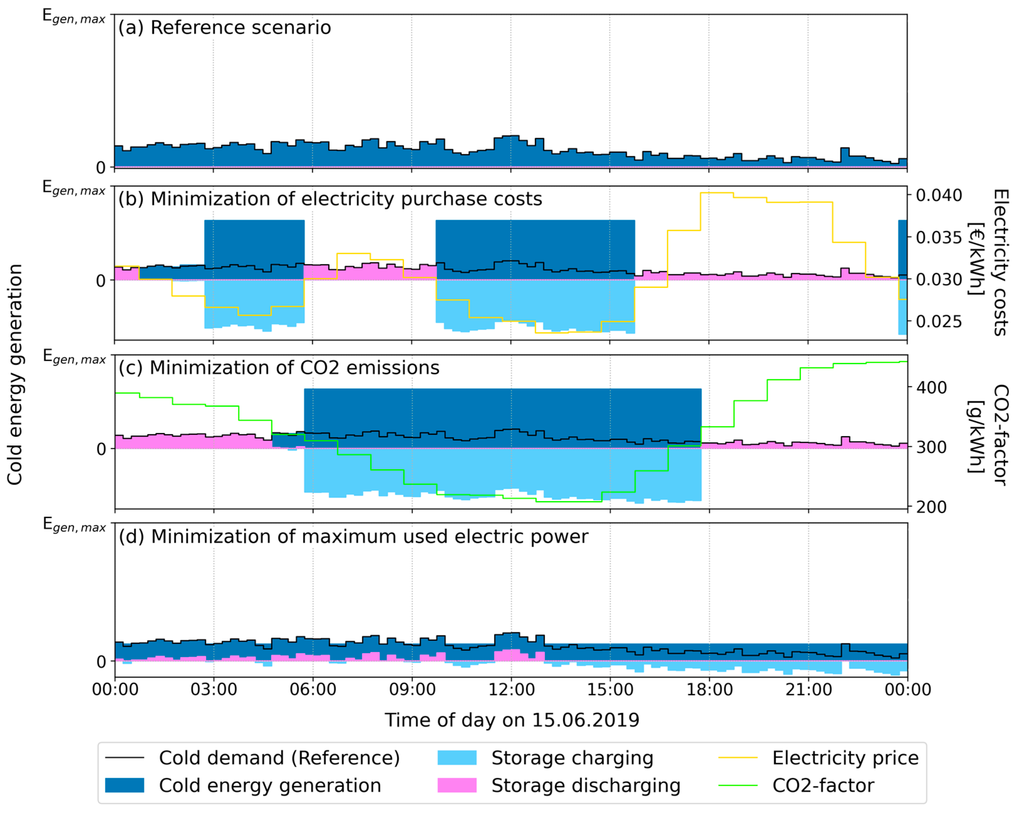
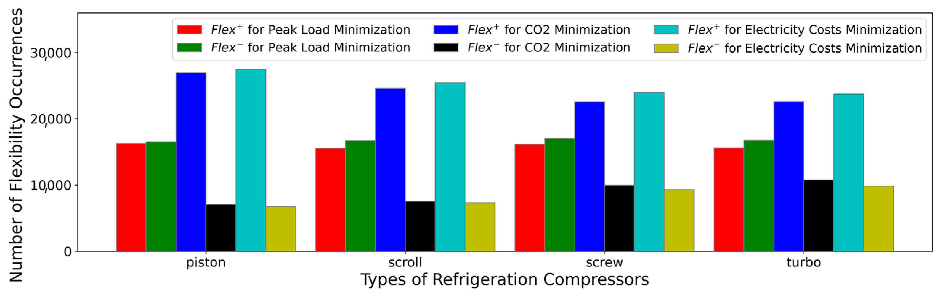
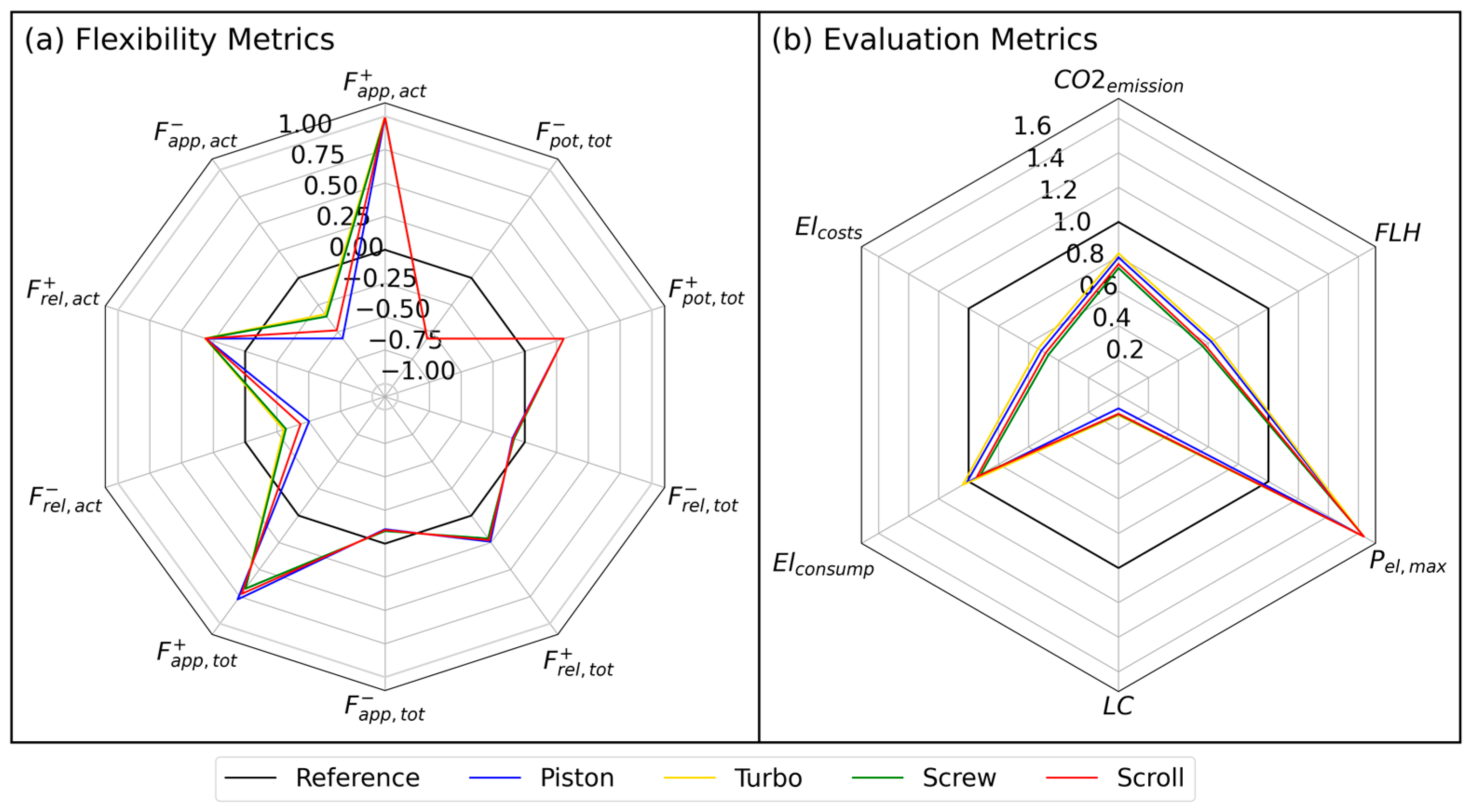
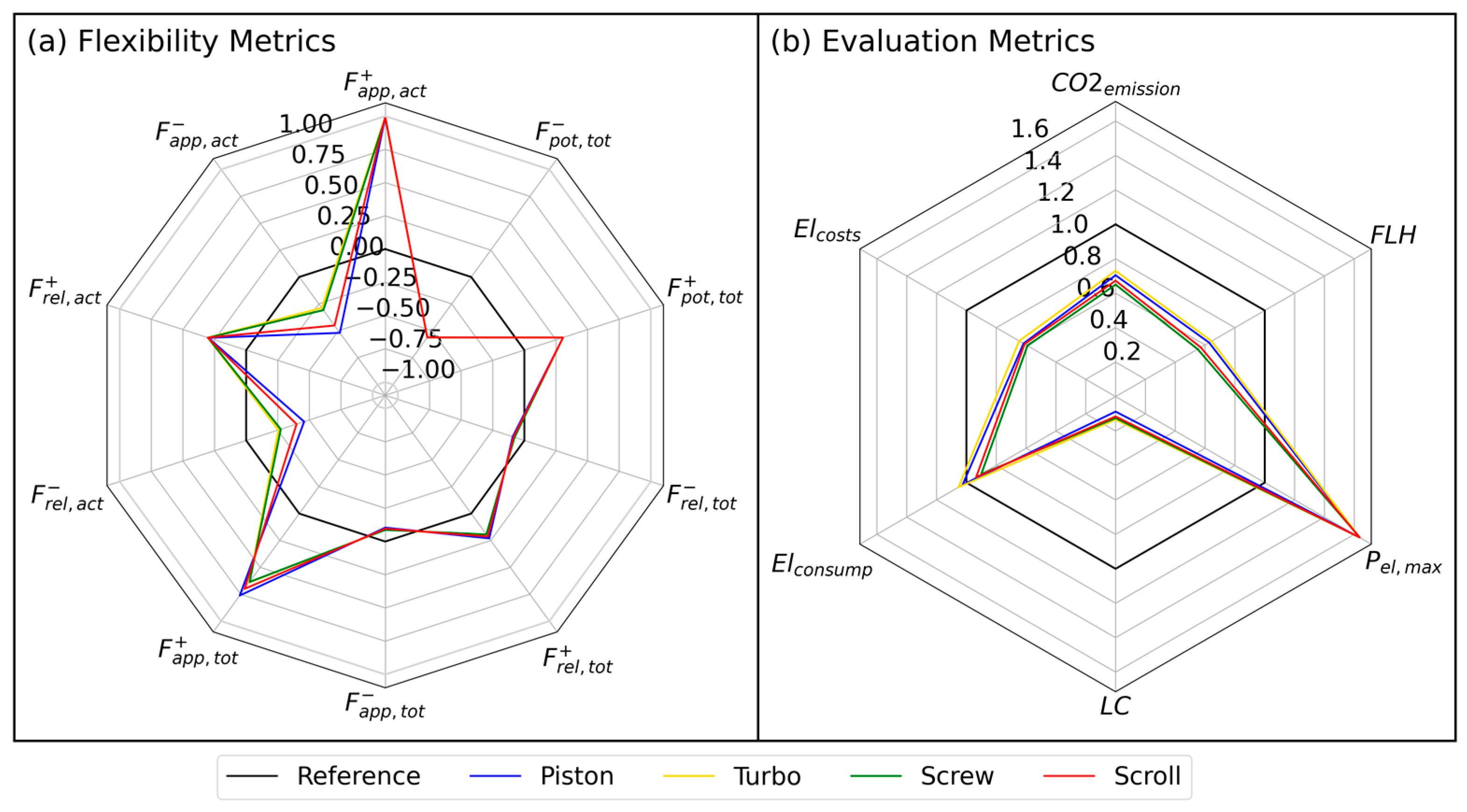
Reduction of electricity purchase costs up to 50%;

-

Reduction of CO₂ emissions between 25–30%;

-

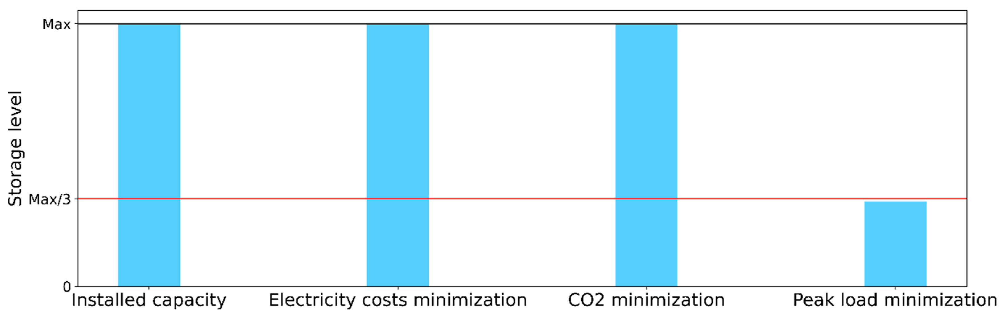
Reduction of electric peak load about 50%;

-

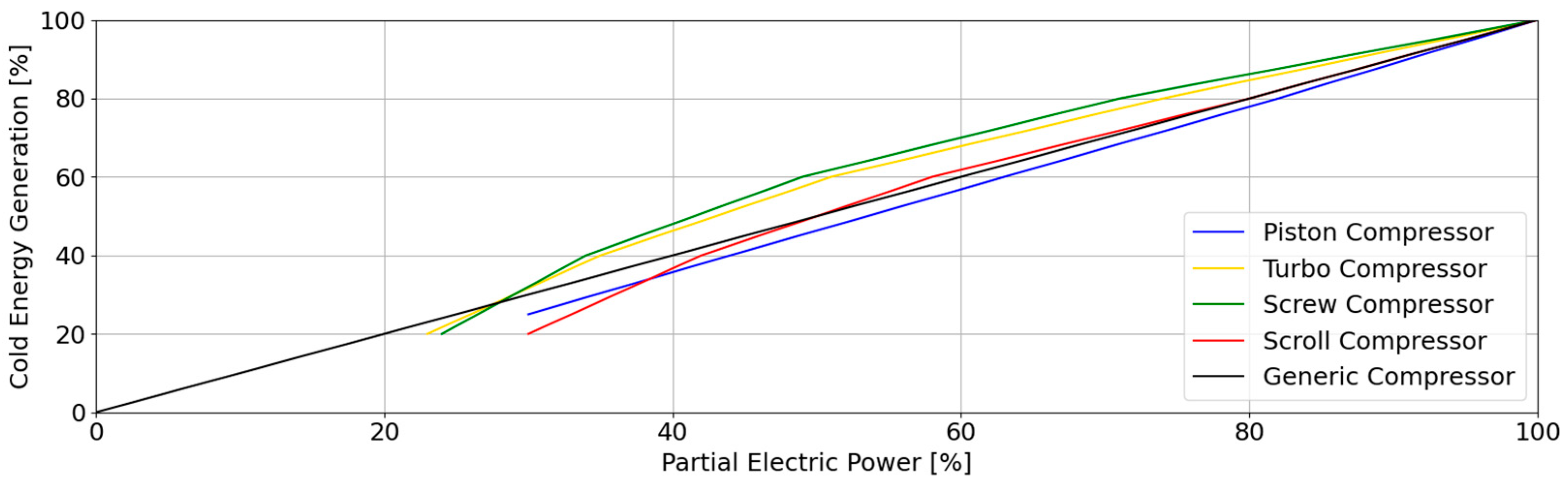
Screw compressors are the most favorable refrigeration compressor type for a goal-oriented flexible operation.

Whereas a high degree of flexibility was required to minimize electricity costs and CO₂ emissions due to the necessity of generating and storing high levels of excess energy in low-cost periods for later use in high-cost periods, minimizing the peak load was possible with much less flexibility via much a smaller electric peak load and storage fill level. Therefore, it can be concluded that a cold warehouse can be potentially operated with a high degree of flexibility if necessary and could be used for DSM purposes. Moreover, almost all types of refrigeration compressors show a similar pattern for positive flexibility, while piston compressors show the highest negative flexibility, followed closely by scroll compressors. Nevertheless, a higher level of flexibility does not necessarily lead to better goal-based optimization results. Screw compressors, for example, can be concluded as the most favorable refrigeration compressor type for all the three goals, as they delivered the lowest CO₂ emissions, electricity costs, and even peak loads, although they did not show as much negative flexibility as piston or scroll compressors. In fact, flexibility merely shows the level of change an energy system or its components need to undergo to deliver the optimal results, meaning one plant configuration may need much less flexibility to deliver the same results than another. In addition, the optimal results always depend on the designated goal. For example, achieving the goals “minimization of electricity costs” and “minimization of CO₂ emissions” largely depended on the availability of a high excess energy generation capacity and a very large efficient energy storage, as it is more favorable to generate and store excess cold energy in large amounts in low-cost periods. This is, however, not true for the goal “minimization of peak load”, for which smaller compressors and a lower energy storage capacity would suffice to achieve the optimal results. What is more is that positive flexibility occurred more frequently for the goals “minimization of electricity costs” and “minimization of CO₂ emissions”, as large amounts of excess energy that were stored in a shorter period were discharged to meet the demand over a longer period. This could be because the demand in a single interval was comparatively much smaller than the installed energy generation capacity and storage capacity, allowing the energy generation system to store enough excess energy in a short time window to meet the aggregate demand of a much larger window. However, this was not the case for the minimization of peak load, where charge and discharge patterns occurred at a very similar frequency to help the compressors mainly in high-demand periods. Additionally, it can be seen that positive flexibility was generally larger than negative flexibility, which was due mainly to the fact that positive flexibility had a higher frequency than negative flexibility, and the ratio of the actual discharged energy to the maximum feasible dischargeable energy was larger than the ratio of the actual excess energy to the maximum feasible excess energy.

To sum up, the interpretation of flexibility is not a very straight-forward task. Two energy systems may generate the same amount of CO₂ emissions after being flexibly operated, but this does not mean that they possess the same degree of flexibility, as one energy system may have needed to undergo more changes to emit the same amount of CO₂. Moreover, the maximum flexibility potential of an energy system cannot be found without pursuing a goal, as a mere flexible operation of an energy system does not provide any useful information. Additionally, the flexible operation of an energy system is substantially limited by the pursuit goal. As was seen, much less flexibility was required for minimizing the peak load than for minimizing the electricity costs. Therefore, careful wording is required to evaluate flexibility. As an example, it can be stated that an energy system needs a certain degree of flexibility to realize its maximum potential to minimize its CO₂ emissions, or this is the maximum amount of CO₂ that an energy system can emit if it is operated flexibly. As the focus of this study was to provide a theoretical quantification of flexibility potential of cold supply systems, further practical studies were not conducted in this project. Consequently, a central question for future research would be how the theoretical flexibility potential of cold supply systems can be realized in practice, where real energy storages with a lower efficiency, inaccurate forecasted prices, and technical as well as contractual and organizational obstacles exist. It is also of crucial importance to carry out sensitivity calculations for the optimized dimensioning of refrigeration compressors and cold energy storage, taking into account not only the operating costs but also investment costs or all life cycle costs.

References

1. Basit, M.A.; Dilshad, S.; Badar, R.; Sami ur Rehman, S.M. Limitations, challenges, and solution approaches in grid-connected renewable energy systems. Int. J. Energy Res. 2020, 44, 4132–4162. [Google Scholar] [CrossRef]
2. Reynders, G.; Amaral Lopes, R.; Marszal-Pomianowska, A.; Aelenei, D.; Martins, J.; Saelens, D. Energy flexible buildings: An evaluation of definitions and quantification methodologies applied to thermal storage. Energy Build. 2018, 166, 372–390. [Google Scholar] [CrossRef]
3. Osička, J.; Černoch, F. European energy politics after Ukraine: The road ahead. Energy Res. Social. Sci. 2022, 91, 102757. [Google Scholar] [CrossRef]
4. Ashok, S.; Banerjee, R. An optimization mode for industrial load management. IEEE Trans. Power Syst. 2001, 16, 879–884. [Google Scholar] [CrossRef]
5. Sinsel, S.R.; Riemke, R.L.; Hoffmann, V.H. Challenges and solution technologies for the integration of variable renewable energy sources—A review. Renew. Energy 2020, 145, 2271–2285. [Google Scholar] [CrossRef]
6. Denholm, P.; Hand, M. Grid flexibility and storage required to achieve very high penetration of variable renewable electricity. Energy Policy 2011, 39, 1817–1830. [Google Scholar] [CrossRef]
7. Moslehi, K.; Kumar, R. A Reliability Perspective of the Smart Grid. IEEE Trans. Smart Grid 2010, 1, 57–64. [Google Scholar] [CrossRef]
8. Strbac, G. Demand side management: Benefits and challenges. Energy Policy 2008, 36, 4419–4426. [Google Scholar] [CrossRef]
9. Grein, A.; Pehnt, M. Load management for refrigeration systems: Potentials and barriers. Energy Policy 2011, 39, 5598–5608. [Google Scholar] [CrossRef]
10. D’hulst, R.; Labeeuw, W.; Beusen, B.; Claessens, S.; Deconinck, G.; Vanthournout, K. Demand response flexibility and flexibility potential of residential smart appliances: Experiences from large pilot test in Belgium. Appl. Energy 2015, 155, 79–90. [Google Scholar] [CrossRef]
11. Stinner, S.; Huchtemann, K.; Müller, D. Quantifying the operational flexibility of building energy systems with thermal energy storages. Appl. Energy 2016, 181, 140–154. [Google Scholar] [CrossRef]
12. Lund, P.D.; Lindgren, J.; Mikkola, J.; Salpakari, J. Review of energy system flexibility measures to enable high levels of variable renewable electricity. Renew. Sustain. Energy Rev. 2015, 45, 785–807. [Google Scholar] [CrossRef]
13. Lopes, R.A.; Chambel, A.; Neves, J.; Aelenei, D.; Martins, J. A Literature Review of Methodologies Used to Assess the Energy Flexibility of Buildings. Energy Procedia 2016, 91, 1053–1058. [Google Scholar] [CrossRef]
14. Arteconi, A.; Hewitt, N.J.; Polonara, F. State of the art of thermal storage for demand-side management. Appl. Energy 2012, 93, 371–389. [Google Scholar] [CrossRef]
15. Eisenhauer, S.; Marmullaku, D.; Reichart, M.; Sauer, A. Simulationsgestützte Analyse der Energetischen Flexibilisierbarkeit Industrieller Kompressionskälteanlagen; Universität Stuttgart, Institut für Energieeffizienz in der Produktion, Deutsche Kälte- und Klimatagung (DKV-Tagung): Bremen, Germany, 2017. [Google Scholar]
16. Altwies, J.E.; Reindl, D.T. Passive thermal energy storage in refrigerated warehouses. Int. J. Refrig. 2002, 25, 149–157. [Google Scholar] [CrossRef]
17. Tassou, S.A.; Ge, Y.; Hadawey, A.; Marriott, D. Energy consumption and conservation in food retailing. Appl. Therm. Eng. 2011, 31, 2–3. [Google Scholar] [CrossRef]
18. Arteconi, A.; Polonra, F. Demand side management in refrigeration applications. IJHT 2017, 35, S58–S63. [Google Scholar] [CrossRef]
19. Plaum, F.; Ahmadiahangar, R.; Rosin, A.; Kilter, J. Aggregated demand-side energy flexibility: A comprehensive review on characterization, forecasting and market prospects. Energy Rep. 2022, 8, 9344–9362. [Google Scholar] [CrossRef]
20. Kouzelis, K.; Diaz de Cerio Mendaza, I.; Bak-Jensen, B. Probabilistic quantification of potentially flexible residential demand. In Proceedings of the 2014 IEEE PES General Meeting|Conference & Exposition, National Harbor, MD, USA, 27–31 July 2014; IEEE: Piscataway, NJ, USA, 2014; pp. 1–5. [Google Scholar]
21. Groppi, D.; Pfeifer, A.; Garcia, D.A.; Krajačić, G.; Duić, N. A review on energy storage and demand side management solutions in smart energy islands. Renew. Sustain. Energy Rev. 2021, 135, 110–183. [Google Scholar] [CrossRef]
22. Le Dréau, J.; Heiselberg, P. Energy flexibility of residential buildings using short term heat storage in the thermal mass. Energy 2016, 111, 991–1002. [Google Scholar] [CrossRef]
23. Reynders, G.; Nuytten, T.; Saelens, D. Potential of structural thermal mass for demand-side management in dwellings. Build. Environ. 2013, 64, 187–199. [Google Scholar] [CrossRef]
24. Nuytten, T.; Claessens, B.; Paredis, K.; van Bael, J.; Six, D. Flexibility of a combined heat and power system with thermal energy storage for district heating. Appl. Energy 2013, 104, 583–591. [Google Scholar] [CrossRef]
25. Tahersima, F.; Stoustrup, J.; Meybodi, S.A.; Rasmussen, H. Contribution of domestic heating systems to smart grid control. In Proceedings of the IEEE Conference on Decision and Control and European Control Conference, Orlando, FL, USA, 12–15 December 2011; IEEE: Piscataway, NJ, USA, 2011; pp. 3677–3681. [Google Scholar]
26. Weiß, T.; Rüdisser, D.; Reynders, G. Tool to Evaluate the Energy Flexibility in Buildings—A Short Manual: IEA EBC Annex 67 Project Energy Flexible Buildings; AEE INTEC: Gleisdorf, Austria, 2019. [Google Scholar]
27. De Coninck, R.; Helsen, L. Quantification of flexibility in buildings by cost curves—Methodology and application. Appl. Energy 2016, 162, 653–665. [Google Scholar] [CrossRef]
28. Junker, R.G.; Azar, A.G.; Lopes, R.A.; Lindberg, K.B.; Reynders, G.; Relan, R.; Madsen, H. Characterizing the energy flexibility of buildings and districts. Appl. Energy 2018, 225, 175–182. [Google Scholar] [CrossRef]
29. Vandermeulen, A.; van der Heijde, B.; Helsen, L. Controlling district heating and cooling networks to unlock flexibility: A review. Energy 2018, 151, 103–115. [Google Scholar] [CrossRef]
30. Jin, X.; Wu, Q.; Jia, H. Local flexibility markets: Literature review on concepts, models and clearing methods. Appl. Energy 2020, 261, 114387. [Google Scholar] [CrossRef]
31. Graßl, M.A. Bewertung der Energieflexibilität in der Produktion. Ph.D. Thesis, Universität München, Munich, Germany, 2014. [Google Scholar]
32. Ulbig, A.; Andersson, G. Analyzing operational flexibility of electric power systems. Int. J. Electr. Power Energy Syst. 2015, 72, 155–164. [Google Scholar] [CrossRef]
33. Kondziella, H.; Bruckner, T. Flexibility requirements of renewable energy based electricity systems—A review of research results and methodologies. Renew. Sustain. Energy Rev. 2016, 53, 10–22. [Google Scholar] [CrossRef]
34. Nalini, B.K.; Eldakadosi, M.; You, Z.; Zade, M.; Tzscheutschler, P.; Wagner, U. Towards Prosumer Flexibility Markets: A Photovoltaic and Battery Storage Model. In Proceedings of the 2019 IEEE PES Innovative Smart Grid Technologies Europe (ISGT-Europe), Bucharest, Romania, 29 September–2 October 2019; IEEE: Piscataway, NJ, USA, 2019; pp. 1–5. [Google Scholar]
35. Li, R.; Satchwell, A.J.; Finn, D.; Christensen, T.H.; Kummert, M.; Le Dréau, J.; Lopes, R.A.; Madsen, H.; Salom, J.; Henze, G.; et al. Ten questions concerning energy flexibility in buildings. Build. Environ. 2022, 223, 109461. [Google Scholar] [CrossRef]
36. Huber, M.; Dimkova, D.; Hamacher, T. Integration of wind and solar power in Europe: Assessment of flexibility requirements. Energy 2014, 69, 236–246. [Google Scholar] [CrossRef]
37. Fischer, D.; Wolf, T.; Wapler, J.; Hollinger, R.; Madani, H. Model-based flexibility assessment of a residential heat pump pool. Energy 2017, 118, 853–864. [Google Scholar] [CrossRef]
38. Oldewurtel, F.; Sturzenegger, D.; Andersson, G.; Morari, M.; Smith, R.S. Towards a standardized building assessment for demand response. In Proceedings of the 52nd IEEE Conference on Decision and Control, Florence, Italy, 10–13 December 2013; IEEE: Piscataway, NJ, USA, 2013; pp. 7083–7088. [Google Scholar]
39. Brouwer, A.S.; van den Broek, M.; Seebregts, A.; Faaij, A. Operational flexibility and economics of power plants in future low-carbon power systems. Appl. Energy 2015, 156, 107–128. [Google Scholar] [CrossRef]
40. Saarinen, L.; Dahlbäck, N.; Lundin, U. Power system flexibility need induced by wind and solar power intermittency on time scales of 1–14 days. Renew. Energy 2015, 83, 339–344. [Google Scholar] [CrossRef]
41. Finck, C.; Li, R.; Kramer, R.; Zeiler, W. Quantifying demand flexibility of power-to-heat and thermal energy storage in the control of building heating systems. Appl. Energy 2018, 209, 409–425. [Google Scholar] [CrossRef]
42. Riaz, S.; Mancarella, P. Modelling and Characterisation of Flexibility from Distributed Energy Resources. IEEE Trans. Power Syst. 2022, 37, 38–50. [Google Scholar] [CrossRef]
43. Reynders, G.; Diriken, J.; Saelens, D. Generic characterization method for energy flexibility: Applied to structural thermal storage in residential buildings. Appl. Energy 2017, 198, 192–202. [Google Scholar] [CrossRef]
44. oemof. A Modular Open Source Framework to Model Energy Supply Systems. 2022. Available online: https://oemof.org/ (accessed on 14 November 2023).
45. Market Data|EPEX SPOT. 2022. Available online: https://www.epexspot.com/en/market-data (accessed on 14 November 2023).
46. Agorameter. 2023. Available online: https://www.agora-energiewende.de/service/agorameter/chart/power_generation/28.02.2023/03.03.2023/today/ (accessed on 12 February 2023).
47. Sprenger, E.; Recknagel, H.; Albers, K.-J. Taschenbuch für Heizung + Klimatechnik; RECKNAGEL: Munich, Germany, 2015. [Google Scholar]
48. IKET (Ed.) Pohlmann Taschenbuch der Kältetechnik: Grundlagen, Anwendungen, Arbeitstabellen und Vorschriften; VDE VERLAG: Berlin, Germany, 2018; ISBN 978-3-8007-4149-6. [Google Scholar]
49. Hu, S.-C.; Yang, R.-H. Development and testing of a multi-type air conditioner without using AC inverters. Energy Convers. Manag. 2005, 46, 373–383. [Google Scholar] [CrossRef]
50. Sensfuß, F.; Ragwitz, M.; Genoese, M. The merit-order effect: A detailed analysis of the price effect of renewable electricity generation on spot market prices in Germany. Energy Policy 2008, 36, 3086–3094. [Google Scholar] [CrossRef]
Figure 1. Schematic view of the cold warehouse model developed via oemof.
Energies 17 00085 g001
Figure 2. Partial load behavior of different types of refrigeration compressors: piston [48], turbo and screw compressors [47], scroll compressor [49], and a generic linear compressor.
Energies 17 00085 g002
Figure 3. Optimized operation of the cold warehouse for (a) reference scenario, (b) minimization of electricity costs, (c) minimization of CO2 emissions, and (d) minimization of maximum used electric power on 15 June 2019.
Energies 17 00085 g003
Figure 4. Level of cold energy storage for the three studied goals compared to the storage installed capacity.
Energies 17 00085 g004
Figure 5. Frequency of occurrences of positive and negative flexibility in the optimized operation.
Energies 17 00085 g005
Figure 6. (a) Flexibility metrics and (b) evaluation metrics based on the optimized operation of the cold warehouse for the goal “minimization of electricity costs”.
Energies 17 00085 g006
Figure 7. (a) Flexibility metrics and (b) evaluation metrics based on the optimized operation of the cold warehouse for the goal “minimization of CO2 emissions”.
Energies 17 00085 g007
Figure 8. (a) Flexibility metrics and (b) evaluation metrics based on the optimized operation of the cold warehouse for the goal “minimization of maximum used electric power”.
Energies 17 00085 g008