Abstract
The efficiency of Hybrid Electric Vehicles (HEVs) may be substantially increased if the energy of the exhaust gases, which do not complete the expansion inside the cylinder of the internal combustion engine, is efficiently recovered by means of a properly designed turbogenerator and employed for vehicle propulsion; previous studies, carried out by the same authors of this work, showed a potential hybrid vehicle fuel efficiency increment up to 15% by employing a 20 kW turbine on a 100 HP rated power thermal unit. The innovative thermal unit here proposed is composed of a supercharged engine endowed with a properly designed turbogenerator, which comprises two fundamental elements: an exhaust gas turbine expressly designed and optimized for the application, and a suitable electric generator necessary to convert the recovered energy into electric energy, which can be stored in the on-board energy storage system of the vehicle. In these two parts, the realistic efficiency of the innovative thermal unit for hybrid vehicle is evaluated and compared to a traditional turbocharged engine. In Part 1, the authors present a model for the prediction of the efficiency of a dedicated radial turbine, based on a simple but effective mean-line approach; the same paper also reports a design algorithm, which, owing to some assumptions and approximations, allows a fast determination of the proper turbine geometry for a given design operating condition. It is worth pointing out that, being optimized for quasi-steady power production, the exhaust gas turbine considered is quite different from the ones commonly employed for turbocharging application; for this reason, and in consideration of the required power size, such a turbine is not available on the market, nor has its development been previously carried out in the scientific literature. In the Part 2 paper, a radial turbine geometry is defined for the thermal unit previously calculated, employing the design algorithm described in Part 1; the realistic energetic advantage that could be achieved by the implementation of the turbogenerator on a hybrid propulsion system is evaluated through the performance prediction model under the different operating conditions of the thermal unit. As an overall result, it was estimated that, compared to a reference traditional turbocharged engine, the turbocompound system could gain vehicle efficiency improvement between 3.1% and 17.9%, depending on the output power level, while an average efficiency increment of 10.9% was determined for the whole operating range.
1. Introduction
The continuous growth of global population and the development of emerging economies tend to increase the human consumption of natural resources and the environmental impact of human activities. Among the negative effects of the latter, particularly relevant is the release of greenhouse gases in the atmosphere, which causes the well-known global warming and the related climate change. The European Union addresses this challenge through the European Green Deal, which is a plan to make the EU the first carbon-neutral continent by 2050, passing through the intermediate goal of 55% CO2 emissions cut by 2030 [1]. The data provided by the European Environment Agency (EEA) in 2018 showed that the transport sector is responsible for about 32% of the total CO2 emissions in the European Union [2]. As a consequence, actions are being taken to achieve the reduction in pollutant emissions from road, rail, aviation, and waterborne transport [3]. In this framework, the authors performed a study aimed at investigating and designing a system that allows better exploitation of the chemical energy contained in the fuel used in internal combustion engines. In fact, as widely known, internal combustion engines based on Otto or Diesel cycles do not complete the in-cylinder gas expansion down to atmospheric pressure; as a result, hot and pressurized gas exits the cylinder during the exhaust process, thus reducing by about 19% the energy transfer to the piston. Several solutions have been implemented to recover the unexpanded gas energy; the Atkinson cycle, for instance, allows a theoretical efficiency increase of 19% compared to the Otto cycle with the same compression ratio. There is a major drawback though, as the Atkinson cycle would require an engine displacement four times greater than that of the Otto cycle engine, resulting in a 72% IMEP reduction. The Miller cycle, on the other hand, is meant to provide a compromise between engine efficiency increase and power density depletion; as example, adopting a compression ratio of 14 allows for attaining a theoretical 8% efficiency increase compared to the Otto cycle, with a 25% IMEP reduction. It is also possible to conceive more complex systems that involve turbomachinery, such as turbomechanical and turboelectrical compounding [4,5,6,7,8,9,10,11], and turbocharging. Concerning turboelectrical compounding, the approach usually followed for the automotive application is to install an electrical generator on the turbocharger shaft with the aim to convert into electric power the part of the mechanical power produced by the turbine that is not employed by the turbocompressor [4,5,6,7,8,9]. In all of these cases, maximum efficiency increments within 6% have been attained. In [9], an auxiliary turbogenerator was installed downstream from the first turbine, reaching a maximum fuel economy improvement of 4%. In [10,11], the implementation of an auxiliary turbogenerator in parallel with the main turbocharger allowed for attaining efficiency improvement up to 9%. In these two papers (see also Part 2 [12]), the authors investigated a different arrangement, which is particularly suitable for hybrid propulsion architectures.
The architecture proposed by the authors is an innovative compound system in which a specifically designed exhaust gas turbine connected to a proper electric generator converts the unexpanded exhaust gas energy into electric energy, which is delivered to the vehicle storage system. This energy can then be used for vehicle traction, but also to power the supercharger, which is driven by an independent electric motor. The architecture described is shown in Figure 1, and it is named Separated Electric Compound Engine since the exhaust gas turbine and the compressor are mechanically decoupled, thus letting their operating conditions be independent from each other. Different from the turbomechanical and turboelectrical compound systems already described in the scientific literature [4,5,6,7,8,9,10,11], in the system here proposed the two thermal machines (compressor and turbine) are not connected together, thus ensuring the possibility to control and optimize their operating conditions independently. It derives that the turbine always operates with the maximum mass flow (no wastegate is involved) with the aim to convert as much energy as possible from the exhaust gas, while the compressor is driven only if supercharging is necessary. Moreover, since the rotational speed of the turbine is independent from the engine and from the compressor, it can be optimally controlled and set to the best value acting through the connected generator. In their preliminary studies [13,14], the authors demonstrated that this system is very promising, as it may achieve overall vehicle efficiency advantages up to 15% with respect to a reference hybrid propulsion system of the same nominal overall output power (73.5 kW) equipped with a traditional turbocharged engine. Furthermore, the authors showed that the contribution of the turbogenerator may reach an impressive 33.9% share of the total power generated by the whole system, with maximum power delivered of 20 kW; in this regard, it must be pointed out that in their previous works, the exhaust gas turbine considered was supposed to be optimized for steady-state operation, since in a hybrid propulsion system the thermal engine undergoes small speed and load variations. Quite differently, the turbines usually employed for a turbocharging purpose provide only the power required by the compressor and are designed for unsteady operation on account of the strong speed and mass flow variations, owing to the wide and rapid speed and load variation in the thermal engine. This clarifies that the turbogenerator here considered, and the whole hybrid propulsion system shown in Figure 1, are not commercially available at the moment. The only commercially available products are composed of a radial turbine for turbocharging application connected to an electric generator [15,16,17] and are designed exclusively to supply the electric accessories of traditional vehicles, thus producing maximum output power within 6 kW. Given the lack of adequate references on the market, as indicated in the scientific literature, and in their preliminary studies, the authors considered a constant turbine thermomechanical efficiency ηT,tm (i.e., the product of the total to static isentropic efficiency ηt,s and the mechanical efficiency ηm), i.e., independent of the turbine speed and pressure ratio; more in detail, in their preliminary analysis, the authors considered two different levels of thermomechanical efficiency, namely 0.70 and 0.75. These values are substantially higher than the efficiency of a common turbocharging turbine on account of the more favourable working condition already mentioned, which allows a design strategy aimed at maximizing the efficiency in steady operation, and also permits the control module of the electric generator to operate the turbine at its best efficiency speed ratio, regardless of the power produced. It is also worth noting that in the preliminary evaluations performed [13,14], the efficiency of the electric motor (0.90) employed to drive the supercharger was considered in the evaluation of the power drained by the compressor, since it constitutes an ancillary device, which burdens the overall energy balance of the engine; instead, concerning the turbine, the efficiencies of the electric generator and of the battery charging were not considered coherently with the approach followed for the main thermal engine, whose power output was not reduced by generator efficiency or by battery-charging efficiency; the reason for this approach is that the engine power split (i.e., part to the generator and part to the wheels) should depend on the particular mechanical transmission adopted and was not defined in the evaluation carried out. Moreover, both the generator and the battery-charging efficiency can also be considered the same for the comparative hybrid propulsion system equipped with the traditional turbocharged engine; on account of this, the authors decided to fairly base the comparison on the overall mechanical output power produced. The aim of the work reported in these two papers is to provide a more precise and reliable estimation of the performances of the separated electric compound system by evaluating the turbine efficiency in accordance with its operating condition [12]; this should improve the reliability of the results obtained, which would not be influenced any more by the simplifying assumption used in the preliminary studies, for which the turbine efficiency was assumed to be constant. To this end, the turbine was analysed and designed by means of a simple yet effective mean-line-based approach.
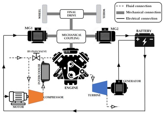
Figure 1.
Schematic representation of the separated electric compound system.
In this paper, the authors focused on radial turbines instead of multistage axial turbines with a view to a good compromise between efficiency and overall machine size [18,19,20]. As the first step, the authors evaluated the Mass Flow Parameter (MFP) that resulted in one of the preliminary studies [13], in order to identify the most suitable kind of turbine to employ in this application.
As can be observed in Figure 2, the separated electric compound engine requires multiple swallowing curves as a function of the pressure ratio βT. For this reason the authors considered a variable nozzle turbine, capable to allow multiple mass-flow curves through the variation in the nozzle angle [21].
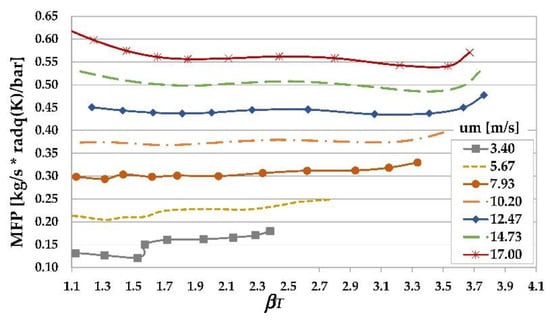
Figure 2.
Operating points of the exhaust gas turbine for the separated electric compound engine studied in [4] (mass flow parameter as a function of the turbine pressure ratio βT).
In the next part of the paper, the authors first present the mean-line prediction model algorithm used to evaluate the turbine performance for all the operating conditions of pressure ratio βT and rotational speeds n (and consequent mass flow G). Successively, the design algorithm was adopted to determine the main geometric dimensions of the turbine at the design-operating condition, as presented. As a final step, the authors present the realistic performance of the separated electric compound engine evaluated by means of a 1D turbine performance prediction model applied to the design geometry.
2. Radial Turbine Performance Calculation Model
As mentioned, the model adopted for the prediction of the turbine performance is based on mean-line analysis, according to which the flow is one-dimensional and is calculated at the mean radius of the turbomachinery stage, where the fluid properties are evaluated as reasonable average values across the full blade span. Mean-line analysis can provide good estimation of the geometry and flow parameters through a turbomachine in relatively short times. The authors adopted this approach since it represents the best solution for a preliminary design and performance analysis of a turbomachine, and constitutes the best compromise between reliability of the results and computational times. Indeed, as a final design step, more detailed aerodynamic performance evaluation could be accomplished by means of CFD analysis, once the appropriate turbine geometry has been defined through mean-line analysis. Figure 3 shows a schematic representation of the whole radial turbine, which includes the volute (from Section 1 to Section 2), the distributor nozzle (from Section 2 to 3), and the rotor (from Section 4 to 5).
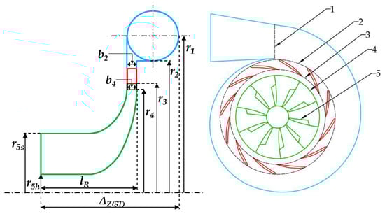
Figure 3.
Schematic representation of turbine geometry, the numbers refer to the following main flow sections: (1) volute inlet; (2) nozzle inlet; (3) nozzle outlet; (4) rotor inlet; (5) rotor exit.
In order to realistically assess the turbine efficiency, it was necessary to take into account the actual operating conditions; most of the time, in effect, the turbine does not operate at the design condition, since the pressure ratio and/or the rotational speed may be substantially different from the design values. For a given turbine geometry, the off-design operation will cause different mass flow rates and velocity triangles with respect to the design condition, and as a consequence, the turbine will exhibit a different overall performance, i.e., different output power and efficiency with respect to the design point. With the aim to calculate the performance of the turbine for any possible operating condition, it was necessary to evaluate the energy losses connected to the flow inside the machine by identifying the entropy generation mechanisms and quantifying their contribution in every phase of the fluid flow through the machine. The major contributions to the entropy generation [19,21] are caused by incidence losses, passage losses (due to friction, secondary flow and flow separation), tip leakage flow, and trailing edge losses, which occur in the internal blade passages in each of the elements of the turbomachine (volute, nozzle and rotor). All of these losses are conveniently quantified in terms of differences between the actual static enthalpy at the exit of a stage and that of the equivalent ideal isentropic process.
2.1. Analysis of the Volute
The purpose of the volute is to distribute the flow around the periphery of the turbine providing uniform mass flow rate and uniform static pressure at the volute exit, thus ensuring the proper exploitation of each rotor blade passage and avoiding unsteady radial loading of the rotating system.
The static temperature at volute inlet T1 can be calculated from the application of the first law of thermodynamics to a perfect gas:
where c1 is the absolute gas velocity at the volute inlet Section 1, and is the specific heat at constant pressure evaluated at the average temperature = (TT1 + T1)/2 through the use of the Shomate equation, and the coefficients available in the NIST Chemistry WebBook [22]. It is worth noting that Equation (1) implies an iterative calculation, since requires the value of T1, which is the output of the equation. As a starting value, was assumed. Analogous iterations have been carried out for similar evaluations performed in this paper.
Since for any given turbine pressure ratio βT = PT1/P5 and rotor speed n, the pressure levels in the Section 1, Section 2, Section 3 and Section 4 (i.e., P1, P2, P3, and P4) are not known a priori, all the absolute velocities in the same sections are initially unknown; for this reason, each calculation procedure was started assuming an initial first attempt value of 100 m/s for each of the unknown absolute velocities (c1, c2, c3, and c4); the values of these velocities were then updated by successive iterations performed with the aim to obtain the mass-flow convergence on all the turbine sections.
Assuming an isentropic expansion from the total condition upstream from the turbine (gas pressure PT1 and temperature TT1) to the static condition, it was possible to calculate the static pressure at the volute inlet as:
where is the mean isentropic coefficient evaluated at the average temperature :
where, according to Meyer’s relation, the specific gas constant R′ is the difference between the constant pressure and the constant volume specific heats cp and cv. It is worth pointing out that, in the case of the isentropic transformation, the average temperature = (TT1 + T1,is)/2 should be considered; however, since the difference between T1 and T1,is not relevant, it results that the difference between and is negligible (less than 0.01%), as is the difference between and ; the same conclusion is obtained considering the turbine nozzle and the rotor, where the enthalpy drops are higher; according to this observation the authors adopted the approximation to use the average temperature of the actual evolution in place of the average temperature of the isentropic evolution when calculating the thermochemical properties of the gas, i.e., the specific heat at constant pressure and the isentropic coefficient.
The static density of the gas at the volute inlet ρ1 was then calculated by means of the ideal gas law as function of P1 and T1 as:
Additionally, the mass-flow rate at the volute inlet G1 is:
where A1 is the inlet volute area. The absolute gas velocity c1 was then corrected with the aim to reduce the difference between the mass flow at the volute inlet G1 and outlet G2 (whose calculation is shown below), which is considered a mass-flow error:
where fC is the factor adopted for the absolute velocity iterative corrections; the same approach was followed for the correction of all the other absolute velocities, each one correlated to a proper mass-flow error; once all the mass-flow errors reach a negligible value (i.e., less than 0.1% of the mass-flow), the solution is considered the final and the calculation procedure is stopped. The convergence on the mass flow was reached acting on the absolute velocities (c1, c2, c3, and c4) rather than on the static pressure levels (P1, P2, P3, and P4) since the iterative correction performed on the static pressure values revealed some calculation instabilities.
Concerning the flow within the turbine volute, the most common assumption usually made is to consider a free vortex evolution; various extensions to the free vortex model, however, have been proposed in the scientific literature to reproduce the actual flow conditions, which are affected by friction, secondary flows, and mixing of the mainstream flow with outer fluid in the proximity of the outlet section. Loss correlations and coefficients may be used to account for deviations from the ideal evolution. Kastner and Bhinder [23] represented the volute loss as a friction loss using conventional pipe-flow correlations. As proposed by Baines [21], this loss item can be considered as the difference between the actual static enthalpy at exit from the volute and that of the equivalent isentropic process:
where is the mean passage velocity (average value between inlet and outlet velocity), Lhyd,vol and Dhyd,vol are the hydraulic length and diameter of the volute respectively, while the coefficient of friction Cf is defined as:
where is the mean kinematic viscosity of the fluid between the inlet and outlet of the volute. The free vortex evolution can be hence modified to include the effects of shear stresses due to friction by means of the following relation:
which gives the tangential component of the absolute velocity at the volute outlet c2u. This correlation is based on an analysis performed by Stanitz [24] on the flow in the vaneless diffuser of a compressor, but being an analysis based on fundamental control volume, it could be adapted to the flows in the turbine volutes. Obviously, the volute loss produces a reduction in the actual fluid velocity at the volute outlet with respect to the ideal evolution, as shown by the simple application of the first law of thermodynamics between volute inlet and outlet sections:
where ΔHis(vol) and ΔHre(vol) are the isentropic and the actual enthalpy drop in the volute, respectively. As already mentioned, however, the pressure level at the volute outlet P2 is initially unknown, which means that the isentropic enthalpy drop is also unknown and therefore the absolute velocity c2 as well, which, in turn, is required for the calculation of the volute loss. The calculation procedure is hence based on successive iterative approximation; the initial value of 100 m/s was assumed for the absolute velocity at nozzle inlet c2, which, in turn, allowed for evaluating the gas temperature at the volute outlet T2 by the application of the first law of thermodynamics:
and the consequent actual enthalpy drop in the volute ΔHre(vol):
Considering the isentropic transformation, the static pressure at nozzle outlet was evaluated as:
where the isentropic enthalpy drop is obtained as the sum of the actual enthalpy drop (Equation (12)) and the volute loss (Equation (7)):
As already discussed, the mean constant pressure specific heat and the mean isentropic coefficient were both evaluated at the average temperature = (T1 + T2)/2. As done for the volute inlet (see Equation (4)), the fluid density at the volute outlet section ρ2 was evaluated though the application of the ideal gas law as a function of the pressure P2 and the temperature T2. The mass flow through the volute outlet section G2 could be hence calculated as:
where the meridional component of absolute velocity at volute outlet c2m was evaluated as a function of the tangential component of the absolute velocity c2u obtained by Equation (9):
Again, the absolute velocity at the volute outlet c2 was corrected with the aim to reduce the mass-flow error between the volute outlet and nozzle outlet, i.e., (G2 − G3):
Once the value of the absolute velocity at volute outlet c2 is updated, then the entire calculation procedure from Equation (7) to Equation (17) is repeated until the mass-flow error (G2 − G3) becomes negligible (i.e., less than 0.1% of G2).
2.2. Analysis of the Nozzle
The nozzle consists of an annular ring of vanes that set the angle of approach of the working fluid to the rotor and it works in conjunction with the volute to accelerate the fluid. As in the case of the volute, nozzle losses ultimately lead to a reduction in outlet velocity compared to the ideal evolution. It is possible to distinguish nozzle passage losses and nozzle incidence losses. The nozzle passage loss is mainly caused by the action of friction forces between the flow and the nozzle blade’s solid surface [25], which was determined by the following equation:
where Lhyd,nozzle and Dhyd,nozzle are the hydraulic length and diameter of the nozzle, respectively, is the mean passage velocity (average value between nozzle inlet and outlet), and f is the friction factor, evaluated as:
where is the average Reynolds number between the nozzle inlet and outlet, while RR represents the wall relative roughness, for which the value of 0.0002 m is suggested by Suhrmann et al. [26].
The nozzle incidence loss, on the other hand, arises whenever there is a difference between the fluid-dynamic nozzle inlet angle α2,f and the nozzle geometric inlet angle α2,g; a simple yet effective correlation for the calculation of the nozzle incidence loss is:
As already observed in the case of the volute, the absolute velocity at nozzle outlet c3 is related to the isentropic enthalpy drop in the nozzle ΔHis(nozzle), to the actual enthalpy drop ΔHre(nozzle) and to the losses Δhp(nozzle) and Δhi(nozzle) by the first law of thermodynamics applied between the inlet and outlet sections of the nozzle (i.e., Section 2 and Section 3 of Figure 3):
Additionally, in this case, because the static pressure at the nozzle exit P3 and the isentropic enthalpy drop are initially unknown, the absolute velocity at the nozzle outlet c3 could not be evaluated through Equation (21); the calculation procedure was also based on a successive iterative approximation in this case, adopting a first attempt value of 100 m/s also for the absolute velocity c3. The static temperature at nozzle outlet T3 was hence calculated as:
and the related actual enthalpy drop in the nozzle:
The static pressure P3 at nozzle outlet was obtained through the isentropic transformation:
where the isentropic enthalpy drop ΔHis(nozzle) was obtained from the actual enthalpy drop and the losses in the nozzle:
The static density of the fluid at nozzle outlet ρ3 was evaluated by applying the ideal gas law (see Equation (4)) as a function of the temperature T3 and pressure P3, thus allowing evaluation of the mass flow at the nozzle exit G3:
where c3m is the meridional component of the gas velocity in the nozzle outlet section:
and A3 the flow section normal to c3m. As already carried out for the volute, the absolute velocity c3 was corrected on the basis of the mass-flow error:
and hence the calculation procedure from Equation (18) to Equation (28) was repeated until the mass-flow convergence was reached.
2.3. Analysis of the Nozzle–Rotor Interspace
In a variable nozzle turbine, the swallowing capacity is controlled though the variation in the nozzle passage section, which is obtained by the rotation of the nozzle blades; the lower mass flows can be obtained adopting small opening angles; increasing the opening angles allows the turbine to swallow higher mass flows. For this reason, a radial gap Δr between the nozzle exit radius r3 and the rotor inlet radius r4 is necessary (see Figure 4) to allow the nozzle blades to rotate without causing any impact on the rotor.
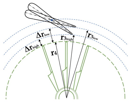
Figure 4.
Radial gap between nozzle outlet section (radius r3) and rotor inlet section (radius r4).
As can also be observed in Figure 4, the radial gap increases when the nozzle blades reduce the opening angle, i.e., when the mass flow is reduced. This radial gap generates a limited interspace between the nozzle outlet (Section 3) and rotor inlet (Section 4), where it is plausible to assume an ideal free vortex evolution, according to which:
where the absolute velocity of the fluid at the rotor inlet c4 is related to the isentropic enthalpy drop in the radial gap ΔHis(gap):
As in the previous cases, being initially unknown, the static pressure at the rotor inlet P4, and hence the isentropic enthalpy drop in the radial gap, the absolute velocity c4 could not be evaluated through Equation (30); an iterative calculation procedure was employed in this case, also adopting a first attempt value of 100 m/s for the absolute velocity c4. The static temperature at the rotor inlet T4 was then calculated as:
The static pressure P4 could be instead obtained through the isentropic evolution from the nozzle exit (condition 3) to rotor inlet (condition 4):
The density of the fluid at the rotor inlet could be hence calculated by the application of the ideal gas law:
which, in turn, allowed calculation of the mass flow at the rotor inlet G4:
where A4 is the flow passage section at the rotor inlet, while the meridional component of the absolute velocity c4m was obtained as:
The absolute velocity c4 at rotor inlet was hence corrected on the basis of the mass-flow error (G4 − G5):
where G5 is the mass flow through the outlet section from the rotor. The calculation procedure from Equation (29) to Equation (36) was repeated until the mass-flow convergence was obtained.
2.4. Analysis of the Rotor
The rotor is composed of a set of rotating blades that constitute a rotating ring of vanes, conceived to transform part of the fluid enthalpy and kinetic energy into mechanical work, which, in turn, is transferred to the rotating shaft. In a moving stage, multiple entropy generation mechanisms contribute to losses; the loss models mainly adopted in the scientific literature when managing the rotor of a radial turbine are: rotor incidence loss, passage loss, clearance loss, disc windage loss, and trailing edge loss [18,19,20].
The rotor incidence loss is related to the incidence of the fluid flows approaching the rotor passage; according to the mostly employed model, described by NASA [27], the enthalpy variation Δhin associated with the rotor incidence loss depends on the difference between the actual fluid-dynamic angle β4,f and the optimum incidence angle β4,opt:
where w4 represents the relative velocity of the fluid at the rotor inlet; it is worth mentioning that the optimum angle β4,opt is different from the geometric angle β4,g due to the motion that the rotor induces in the flow approaching the blades. The optimum angle β4,opt can be evaluated on the basis of the optimal tangential component of relative velocity w4u,opt:
where
The optimal tangential component of the absolute velocity c4u,opt in turn can be evaluated as a function of the peripheral linear velocity at the rotor inlet u4 by means of an empirical equation proposed by Stanitz [28]:
Hence, it results that the optimum angle β4,opt can be evaluated as:
The rotor passage loss is a generic term aimed to quantify the losses due to friction and secondary flow processes that occur in the passage through the rotor vanes; the two contributions are usually incorporated into a single enthalpy variation Δhp since there is currently no way to isolate and measure their effects separately. In [21], the rotor passage losses are quantified through:
where Lhyd,R and Dhyd,R are the hydraulic length and diameter of the rotor, respectively, β5 and b5 are the geometric angle and the blade height at rotor outlet, respectively, and chrot is the rotor blade chord, which, according to [21] can be approximated as:
where Kp is a coefficient which, as suggested in [21], should be set to 0.11 on the basis of some experimental data.
The clearance loss is the loss related to the fluid leakage from the rotor blade through the clearance gap between the rotor and its shroud. This loss seems to be affected to a greater extent by the radial clearance εr than by the axial clearance εx, and there appears to be a cross-coupling effect between the two parameters. The authors evaluated the enthalpy variation Δhcl due to the rotor clearance loss as reported in [21]:
where NR is the number of blades in the rotor, Cx and Cr are geometrical parameters, and the three coefficients Kx, Kr, and Kxr should be set to 0.4, 0.75, and −0.3, respectively, as indicated in [21], in agreement with the previously described influences of εr and εx on rotor clearance loss.
The rotor disc windage loss is an external loss that expresses the power loss due to friction between the back face of the turbine disc and the fluid entrapped in the interspace between the rotor and its housing. According to [29], the enthalpy variation connected to the rotor windage loss Δhw can be modelled as:
where is the average fluid density between inlet and outlet section of the rotor, G5 is the turbine mass flow, and the coefficient Kf, as described in [30], depends on the Reynolds number evaluated at the rotor inlet (Section 4 in Figure 3) and on the turbine geometry:
where εb is the clearance between the back face of the turbine disc and its housing, and b4 represents the blade height at rotor inlet.
Lastly, the trailing-edge loss [31] is related to the sudden expansion of the fluid when it passes the trailing edge of the rotor. The expansion is due to the rapid flow section increment caused by the end of the rotor blades. It is worth pointing out that this loss becomes numerically relevant if the fluid velocity is high, i.e., if the relative Mach number M5,rel (evaluated on the basis of the relative velocity at the rotor exit w5) approaches 1. The model here adopted by the authors calculates the enthalpy variation Δht related to the trailing-edge loss as:
where P5 and T5 are the static pressure and temperature at the rotor exit (Section 5), M5,rel is the previously mentioned relative Mach number in Section 5, k and Cp are the isentropic coefficient and the specific heat, respectively (both evaluated at the temperature T5), and ΔPrel is the pressure drop caused by the sudden expansion, which, according to the model adopted [31], is assumed to be proportional to the relative kinetic energy at the rotor exit:
where r5s and r5h are the shroud and hub radii at rotor exit, respectively (see Figure 3), NR the number of blades in the rotor, and t the blade thickness. In the calculation performed on the rotor, the outlet static pressure P5 is known, being part of the boundary conditions adopted (as resumed in Part 2 [12]); the isentropic enthalpy drop in the rotor can be hence calculated as:
Thus, the actual enthalpy drop in the rotor ΔHre(rot) can be obtained:
where Δhrot is the sum of all the losses in the rotor (=Δhin + Δhp + Δhcl + Δhw + Δht) discussed from Equation (37) to Equation (49). The static gas temperature T5 at the rotor outlet is hence:
and the consequent fluid density ρ5 obtained from the ideal gas law:
The actual enthalpy drop in the rotor also allows for calculation of the relative velocity at rotor outlet w5 through the application of the first law of thermodynamics between Section 4 and Section 5, in the relative reference system of the rotor:
where w4 is the relative velocity at the rotor inlet, u4 and u5 are the peripheral linear velocities at the rotor inlet and outlet, respectively. Once calculated, the value of w5 is updated in Equations (48) and (49), thus allowing an iterative solution. The meridional component of the velocity w5 is:
where β5,g is the geometric blade angle at rotor outlet (see Figure 5). The mass-flow rate can be hence calculated:
which, as already mentioned, is employed in Equation (36) for the iterative correction of the absolute velocity at the rotor inlet c4. Since all the losses were expressed in terms of enthalpy variations, it is possible to evaluate the total-to-static isentropic efficiency of the stage as follows:
where the ideal enthalpy drop ΔHid is calculated considering an isentropic expansion from the inlet conditions (PT1, TT1) to the rotor exit static pressure P5:
where
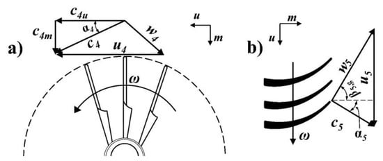
Figure 5.
Velocity triangles (a) rotor inlet; (b) rotor outlet.
2.5. Mechanical Friction Losses
A radial inflow turbine needs at least a journal bearing for shaft rotation and an axial thrust bearing that transfers the axial load of the turbine rotor to the machine frame [32]. The power dissipation in the journal bearing is primarily dependent on bearing geometry, oil viscosity, rotational speed, and oil film thickness. Generally, the frictional power loss in journal bearings can be estimated through Petroff’s equation [33] as:
where µ is the dynamic viscosity of the oil, ω is the rotational speed, L is the bearing length, D is the bearing diameter, and h is the oil film thickness. The bearing diameter D was obtained by designing the shaft for infinite life according to the procedure described in [33], applying the Goodman criterion with a safety factor of 8. The material used for the shaft is 40 NiCrMo 4430 steel, tempered at 540 °C, characterized by yield strength 1080 MPa, and an ultimate tensile strength of 1170 MPa. The oil chosen for this application is Castrol 5W40 and its properties are evaluated at the working temperature of 90 °C. Finally, bearing length L was determined referring to available data for the L/D ratios applied in similar applications.
According to Petroff’s equation, the bearing diameter is the largest influencing factor on power dissipation, followed by the rotational speed. However, decreasing the shaft diameter is not advisable because of the rotor dynamic issues.
The frictional power loss thrust bearings can be described by a modified Petroff’s equation as follows:
where rin,t denotes the inner radius, determined by shaft diameter D; rext,t is the outer radius calculated by making reference to the rext,t/ rin,t ratios used in similar cases; and εth is the axial clearance, for which a value of 0.095 mm was assigned according to [32]. Petroff’s equation reveals that the power dissipation is highly dependent on geometry, as for the journal bearing. Larger bearing contact surfaces result in higher power losses.
3. Design of the Radial Inflow Turbine
In this chapter, the authors describe the procedure adopted to estimate the geometry and flow parameters of the turbomachine for the design condition. The design process is accomplished on the basis of predefined boundary conditions and operating parameters such as total inlet pressure PT1, outlet static pressure P5, total inlet temperature TT1, mass-flow rate G, and rotational speed of the turbine rotor n.
3.1. Rotor Design
Once the turbine design parameters and its boundary conditions have been defined, the first calculation regards the discharge spouting velocity, i.e., the velocity associated with the isentropic enthalpy drop from total inlet pressure PT1 to the final exhaust pressure P5:
where the average temperature is evaluated according to Equations (59) and (60).
Another important parameter is the velocity ratio νs:
Since the value of νs is initially unknown, in the design procedure the first attempt value of 0.5 was assumed, which allows for determining u4 and, in turn, the radius of the rotor inlet section.
In the nominal design condition, the outlet flow should be characterized by a zero swirl at the mean-line analysis, i.e., c5u = 0. As a result, the tangential component c4u of the absolute velocity at rotor inlet could be computed by the application of the Euler equation, once the stage total-to-static efficiency ηt,s is known:
It is obvious that, in the starting phase of the turbine design, the stage total-to-static efficiency ηt,s is unknown (Equation (57)); for this reason, in the design procedure, a first attempt value was obtained by the empirical formula proposed by Aungier [19]:
where the specific speed ns is:
where the volume flow at rotor exit Q5 is the ratio between the mass flow G and the rotor exit density ρ5:
The fluid density at rotor outlet is calculated by means of the ideal gas law on the basis of the static pressure P5 and of the rotor outlet temperature T5, the latter being computed through the application of the first law of thermodynamics from Section 1 to Section 5 on the basis of the actual enthalpy drop ΔHr:
As is usually adopted for radial inward turbines, the inlet blade angle β4g was considered to be 90° in this application. Concerning instead the inlet absolute flow angle α4, in the best efficiency condition, it is substantially a function of the specific speed ns, as shown in [34]. The data reported in [34] have been employed to obtain a numerical correlation [19] used to obtain a first attempt value of the inlet absolute flow angle α4, which is successively updated on the basis of the results:
Equations (66) and (71) allow for determining the meridional component of the fluid velocity at rotor inlet:
The tangential component of relative velocity at the rotor inlet is hence:
which allows for the determination of the fluid-dynamic relative flow angle:
Once the absolute velocity at the rotor inlet is calculated (), it is possible to obtain an approximate evaluation of the thermodynamic state of the fluid at the rotor inlet, as proposed in [19]. Assuming the losses upstream from the rotor to account for about 25% of the total losses and considering a constant density flow, the total pressure at rotor inlet PT4 can be estimated as:
and the static pressure at rotor inlet P4 is hence:
The static enthalpy H4 and the temperature T4 at the rotor inlet may be evaluated as:
The rotor inlet density ρ4 can be then calculated through the application of the ideal gas law, employing the pressure and temperature evaluated in Equations (76) and (78), respectively; the rotor inlet blade height can be hence obtained by the mass-flow rate equation:
and the hub radius at rotor outlet can be obtained as:
where the proportionality constant 0.3 is based on results from the optimization process, as also confirmed in [35]. Following a correlation proposed in [19], the meridional component of the absolute velocity at rotor outlet can be estimated as:
As already mentioned, the zero swirl flow is assumed at the turbine exit (i.e., c5u = 0) in the nominal design condition, thus minimizing the exit kinetic energy losses at the rotor outlet; as a consequence, the absolute velocity at rotor outlet is equal to the meridional component, i.e., c5= c5m. The section area at the rotor outlet is then evaluated:
where the static density at rotor outlet, as noted previously, is calculated by means of the ideal gas law, employing the static pressure P5 (imposed as boundary condition) and the temperature calculated in Equation (70). The exit shroud radius rs5 is therefore:
Then, the rotor outlet mean radius is:
The blade speed at the rotor outlet mean radius is:
According to the zero swirl flow at the rotor outlet, the meridional component of relative velocity coincides with the absolute velocity:
and the tangential component of the relative velocity results:
As a last step, the relative blade angle β5g at the rotor outlet (which in the design condition is equal to the flow angle β5f) is determined:
To complete the geometric design, the rotor axial length is defined through a further empirical correlation provided by [19]:
Glassman [36] introduced an empirical equation for the optimum number of radial inflow turbine rotor blades NR:
whose result, obviously, must be rounded to an integer value.
After the first iteration, Equations (63) to (90) have been updated employing the stage total-to-static efficiency ηt,s obtained from the turbine performance calculation model described in Equation (57) from the previous section. As already mentioned above, the value of νs of the first iteration was imposed equal to 0.5, but successively optimized to obtain the maximum efficiency of the stage.
3.2. Nozzle Design
The nozzle row sizing strategy requires that the nozzle passage width is constant and is identical to the rotor inlet passage width determined from the rotor sizing procedure:
The tangential velocity at the nozzle exit can be calculated by means of the conservation of angular momentum between Section 3 and Section 4:
where the r3 represents the radius at the nozzle exit. As already mentioned and shown in Figure 4, this radius depends on the position of the distributor blades, i.e., on the angle α3: when the distributor blades are closed (i.e., for the minimum mass flow rates), the nozzle outlet flow angle α3 is at its minimum value and hence the radial gap Δr reaches the maximum amplitude. When the mass-flow rates are high, instead, the distributor blades are in a “fully open” position, i.e., with the maximum angle α3, to which corresponds the minimum radial gap Δr. Since in this section the authors are giving the guidelines to define the turbine geometry for a particular design operating condition, the radius at the nozzle exit r3 is given by:
where ΔrD denotes the radial gap value at the design operating condition, which can be roughly obtained as:
It is worth pointing out that once the turbine geometry is defined, the maximum swallowing capacity of the turbine must be verified according to the maximum allowed distributor blade angle α3, which corresponds to a null radial gap; if it results that in this condition the turbine is unable to swallow the required maximum mass-flow rates, then the design must be corrected with a higher value for ΔrD.
For the turbine design procedure, the absolute velocity at nozzle outlet c3 was evaluated assuming the absolute flow angle at nozzle outlet α3 equal to the rotor inlet absolute flow angle α4 (i.e., considering a null radial gap):
The meridional component of absolute velocity is then:
The static enthalpy H3 and the temperature of the gas T3 at the nozzle outlet are computed as:
Since the flow conditions at nozzle inlet are initially unknown, and aiming to induce minimal incidence losses, at the design condition the inlet flow angle is assumed to be equal to the inlet blade angle (i.e., α2f = α2g); moreover, a constant density flow between Section 2 and Section 3 is also assumed, which allows for calculating the meridional component of the absolute velocity at the distributor inlet:
Aungier [19] suggested that the ratio of nozzle inlet to outlet radius r2/r3 lies between 1.1 and 1.7. In this work, the authors adopted a value of 1.3 to obtain a good compromise between performance and overall size of the nozzle. Assuming the symmetrical nozzle blade profile of Figure 6, simple geometric considerations based on the triangle generated by the nozzle geometry (shown in Figure 7), allowed for calculating the nozzle inlet blade angle α2,g as a function of the exit blade angle α3,g:
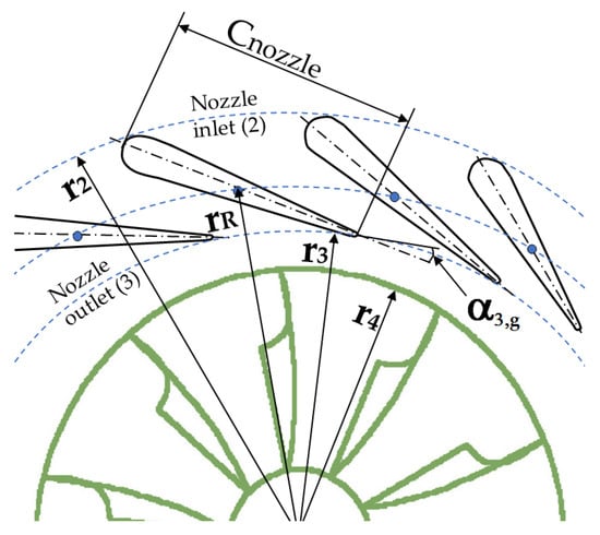
Figure 6.
Geometric representation of the nozzle.
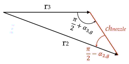
Figure 7.
Schematic representation of nozzle geometry.
Application of Carnot’s theorem for the triangle shown in Figure 7 also allowed for evaluating the length of the nozzle blade chord chnozzle:
Once determined, the distributor inlet flow angle α2, the tangential component of absolute velocity at the nozzle inlet, can be calculated as:
The absolute velocity at nozzle inlet is hence consequently calculated as Since the velocity triangle at the nozzle inlet just calculated is based on the approximate value of c2m obtained from Equation (99), an iterative correction process based on the conservation of mass-flow rate (G2 = G3) is necessary to obtain a more accurate value for c2m. For this purpose, the static temperature and pressure at nozzle inlet are evaluated as:
where, as made previously, both the isentropic coefficient and the specific heat are evaluated at the average temperature of the reference thermodynamic transformation (in this case ). The static density ρ2 of the working fluid at the nozzle inlet can hence be obtained from the ideal gas law as a function of the temperature T2 and pressure P2. At this point the meridional component of the absolute velocity at the distributor inlet is given by:
Equation (106) represents an updated value of the meridional component of absolute velocity at the nozzle inlet, evaluated on the basis of the mass-flow rate swallowing capacity of the section. This value is replaced by the approximate value obtained from Equation (99), thus iteratively recalculating the loop from Equation (100) to Equation (106), until final convergence is achieved.
3.3. Volute Design
The purpose of this section is to describe the analytical procedure adopted by the authors for the design of the main geometric dimensions of the volute, as made in the previous sections; also, in this case, an iterative procedure was repeated until final value convergence was obtained. The volute inlet velocity (Section 1 of Figure 3) is calculated by the conservation of the angular momentum:
Since the value of the radial distance r1 of the volute inlet section from the turbine axis is unknown in the initial phase of the design process, at first attempt it is assumed equal to r2. This assumption allows for evaluation of the static temperature at the volute inlet:
Assuming an isentropic expansion from the total condition to the static condition, it is also possible to calculate the static pressure:
The density of the working fluid is then obtained through the application of the ideal gas law as a function of P1 and T1. The area of the volute inlet section can hence be estimated:
As a general rule, the volute may have an elliptical section, as reported in Figure 8; the axial semi-axis Ax is then:
while the radial distance r1 is:
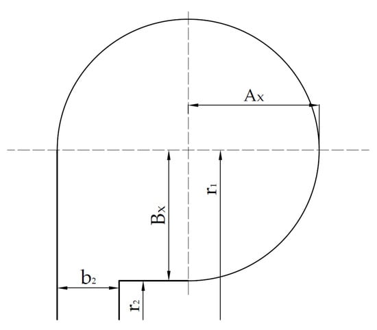
Figure 8.
Inlet volute area geometry.
The radial semi-axis Bx is calculated on the basis of the volute aspect ratio AR:
In this work, the authors adopted an aspect ratio AR = 1, in accordance with the values of 0.75 ≤ AR ≤ 1.5 recommended in [19]. Once the volute section aspect ratio is established, then the calculation loop from Equation (107) to Equation (113) is iteratively repeated until the value of the radius r1 reaches convergence. Therefore, after the volute design is completed, it is possible to estimate the total axial length of the stage as:
3.4. Design Calculation Procedure
With the aim to explain the whole calculation procedure adopted for the radial turbine design, Figure 9 shows a flowchart summarizing the main steps followed by the authors for the definition of the turbine geometry, which are listed below:
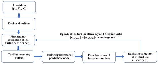
Figure 9.
Flowchart of the design procedure adopted.
The input data (total pressure and temperature at turbine inlet, mass flow) are fed to the algorithm design block.
The algorithm design block estimates a first attempt value for the total-to-static efficiency of the turbine.
The total-to-static efficiency of the turbine is employed by the algorithm design block to define the turbine geometry.
The turbine geometry is fed to the performance prediction model for the realistic evaluation of all the energy losses, giving as a final result the realistic total-to-static efficiency.
The realistic total-to-static efficiency of the turbine is compared with the input efficiency employed in step (3):
If their difference is greater than the convergence value, then the calculation restarts from step (3) by employing the new total-to-static efficiency for the new geometry evaluation.
If their difference is less than or equal to the convergence value, the calculation is stopped and the last turbine geometry is adopted as the final result.
4. Conclusions
The aim of this two-part work is a reliable evaluation of the realistic advantages connected to the implementation of a properly designed turbogenerator for exhaust energy recovery in a hybrid propulsion system. In this Part 1, the authors focused on the design approach to determine the turbine geometry and on the definition of a proper thermomechanical model for the turbine performance estimation. A radial inflow turbine with variable nozzle geometry was adopted in consideration of its capability to allow an adequate control on both mass flow and turbine speed of rotation. The performance evaluation model was based on the simple mean-line approach, with the aim to obtain fast but reliable predictions. With the aim to accurately estimate both the thermodynamic and the mechanical efficiencies, it comprises the most widely recognized energy loss submodels. The design algorithm shares the same structure, but is characterized by a number of assumptions and simplifications that allow a rapid definition of the turbine geometry suitable for the task considered. Both the algorithm and the performance prediction model have been employed in Part 2 [12] to define the turbine geometry according to boundary conditions obtained on a previously studied hybrid propulsion system, and to trace the efficiency map of the turbine. The realistic energetic advantages of the turbocompound engine were hence evaluated [12] on the basis of the realistic turbine efficiencies predicted by the model, and revealed to range between 3.1% and 17.9% depending on the output power level, with a 10.9% average efficiency increment of the realistic turbocompound engine on its best efficiency curve.
Author Contributions
Conceptualization, E.P. and S.C.; methodology, E.P.; software, S.C.; validation, S.C., A.S. and M.C.; formal analysis, M.C.; investigation, A.S.; data curation, S.C.; writing-original draft preparation, S.C.; writing-review and editing, E.P.; visualization, M.C.; supervision, E.P.; funding acquisition, E.P. All authors have read and agreed to the published version of the manuscript.
Funding
Department of Engineering—University of Palermo: FFR_D26_PREMIO_GRUPPO_RICERCA_2020_PIPITONE.
Institutional Review Board Statement
Not applicable.
Informed Consent Statement
Not applicable.
Data Availability Statement
Not applicable.
Conflicts of Interest
The authors declare no conflict of interest.
Symbols and Abbreviations
Symbols
| A | Area | m2 |
| AR | Aspect ratio | - |
| Ax | Axial semi-axis | m |
| b | Blade width | m |
| Bx | Radial semi-axis | m |
| c | Absolute velocity | m/s |
| c0s | Spouting velocity | m/s |
| ch | Chord | m |
| cp | Constant pressure specific heat | |
| cv | Constant volume specific heats | |
| Dhyd | Hydraulic diameter | m |
| EVO | Exhaust valve open | |
| G | Mass flow rate | kg/s |
| H | Specific enthalpy | J/kg |
| IMEP | Indicated mean effective pressure | bar |
| IVC | Inlet valve closure | |
| k | Specific heat ratio | - |
| Lhyd | Hydraulic length | m |
| lr | Rotor axial length | m |
| M | Mach number | - |
| MFP | Mass flow parameter | - |
| n | Rotational speed | rpm |
| NR | Number of rotor blades | - |
| P | Pressure | Pa |
| POW | Power | W |
| r | Radius | M |
| Re | Reynolds number | - |
| RR | Wall relative roughness | M |
| t | Trailing edge blade thickness | M |
| T | Temperature | K |
| u | Peripheral velocity | m/s |
| w | Relative velocity | m/s |
Greek letters
| α | Absolute flow angle | - |
| β | Relative flow angle | - |
| βT | Pressure ratio | - |
| η | Efficiency | - |
| ρ | Density | kg/m3 |
| ω | Rotational speed | rad/s |
| Δh | Enthalpy losses | J/kg |
| ΔH | Enthalpy drop | J/kg |
| ε | Clearance gap | m |
| ν | Kinematic viscosity | m2/s |
| νs | Velocity ratio | - |
Subscripts
| 1 | Total |
| 2 | Nozzle inlet |
| 3 | Nozzle exit |
| 4 | Rotor inlet |
| 5 | Rotor exit |
| a | Axial |
| b | Blade |
| cl | Clearance |
| f | Fluid-dynamic |
| h | Hub |
| id | Ideal |
| in | Incidence |
| is | Isentropic |
| J,B | Journal bearing |
| m | Meridional |
| nozzle | Nozzle |
| p | Passage |
| r | Radial |
| re | Real |
| rel | Relative |
| rot | Rotor |
| s | Shroud |
| t | Trailing edge |
| T | Total |
| tm | Thermomechanical |
| T,B | Thrust bearings |
| t,s | Total-to-static |
| t,t | Total-to-total |
| u | Peripheral |
| vol | Volute |
| w | Windage |
References
- Eurostat, Energy, Transport and Environment Statistics-2020 Edition. Available online: https://ec.europa.eu/eurostat/web/products-statistical-books/-/ks-dk-20-001 (accessed on 14 November 2022). [CrossRef]
- Monitoring CO2 Emissions from Passenger Cars and Vans in 2018; European Environment Agency: Copenhagen, Denmark, 2020. [CrossRef]
- European Commission, Climate Action, EU Action, Transport Emissions, Road Transport: Reducing CO2 Emissions from vehicles, CO2 Emission Performance Standards for Cars and Vans. Available online: https://ec.europa.eu/clima/eu-action/transport-emissions/road-transport-reducing-co2-emissions-vehicles/co2-emission-performance-standards-cars-and-vans_en (accessed on 14 November 2022).
- Pasini, G.; Lutzemberger, G.; Frigo, S.; Marelli, S.; Ceraolo, M.; Gentili, R.; Capobianco, M. Evaluation of an electric turbo compound system for SI engines: A numerical approach. Appl. Energy 2016, 162, 527–540. [Google Scholar] [CrossRef]
- Arsie, I.; Cricchio, A.; Pianese, C.; Ricciardi, V.; De Cesare, M. Evaluation of CO2 reduction in SI engines with Electric Tur-bo-Compound by dynamic powertrain modelling. IFAC-PapersOnLine 2015, 28, 93–100. [Google Scholar] [CrossRef]
- Millo, F.; Mallamo, F.; Pautasso, E.; Ganio Mego, G. The Potential of Electric Exhaust Gas Turbocharging for HD Diesel Engines; SAE Technical Papers; SAE International: Warrendale, PA, USA, 2006. [Google Scholar] [CrossRef]
- Hopmann, U.; Algrain, M. Diesel Engine Electric Turbo Compound Technology; SAE Technical Paper; SAE International: Warrendale, PA, USA, 2003. [Google Scholar] [CrossRef]
- Mohd Noor, A.; Che Puteh, R.; Rajoo, S.; Basheer, U.M.; Md Sah, M.H.; Shaikh Salleh, S.H. Simulation Study on Electric Turbo-Compound (ETC) for Thermal Energy Recovery in Turbocharged Internal Combustion Engine. Appl. Me-Chanics Mater. 2015, 799–800, 895–901. [Google Scholar] [CrossRef]
- Kant, M.; Romagnoli, A.; Mamat, A.M.; Martinez-Botas, R.F. Heavy-duty engine electric turbocompounding. Proc. Inst. Mech. Eng. Part D J. Automob. Eng. 2015, 229, 457–472. [Google Scholar] [CrossRef]
- Cipollone, R.; Di Battista, D.; Gualtieri, A. Turbo compound systems to recover energy in ICE. Int. J. Engi-Neering Innov. Technol. (IJEIT) 2013, 3, 249–257. Available online: https://www.ijeit.com (accessed on 14 November 2022).
- Zhuge, W.; Huang, L.; Wei, W.; Zhang, Y.; He, Y. Optimization of an Electric Turbo Compounding System for Gasoline Engine Exhaust Energy Recovery; SAE Technical Paper; SAE International: Warrendale, PA, USA, 2011. [Google Scholar] [CrossRef]
- Pipitone, E.; Caltabellotta, S.; Sferlazza, A.; Cirrincione, M. Hybrid propulsion efficiency increment through exhaust energy recovery—Part 2: Numerical simulation results. (under review).
- Pipitone, E.; Caltabellotta, S. Efficiency Advantages of the Separated Electric Compound Propulsion System for CNG Hybrid Vehicles. Energies 2021, 14, 8481. [Google Scholar] [CrossRef]
- Pipitone, E.; Caltabellotta, S. The Potential of a Separated Electric Compound Spark-Ignition Engine for Hybrid Vehicle Application. J. Eng. Gas Turbines Power 2022, 144, 041016. [Google Scholar] [CrossRef]
- Michon, M.; Calverley, S.; Clark, R.; Howe, D.; Chambers, J.; Sykes, P.; Dickinson, P.; Clelland, M.; Johnstone, G.; Quinn, R.; et al. Modelling and Testing of a Turbo-generator System for Exhaust Gas Energy Recovery. In Proceedings of the 2007 IEEE Vehicle Power and Propulsion Conference, Arlington, TX, USA, 9–12 September 2007; pp. 544–550. [Google Scholar] [CrossRef]
- Nonthakarn, P.; Ekpanyapong, M.; Nontakaew, U.; Bohez, E. Design and Optimization of an Integrated Turbo-Generator and Thermoelectric Generator for Vehicle Exhaust Electrical Energy Recovery. Energies 2019, 12, 3134. [Google Scholar] [CrossRef]
- Haughton, A.; Dickinson, A. Development of an Exhaust Driven Turbine-Generator Integrated Gas Energy Recovery System (TIGERS®); SAE Technical Paper; SAE International: Warrendale, PA, USA, 2014. [Google Scholar] [CrossRef]
- Rahbar, K. Development and Optimization of Small-Scale Radial Inflow Turbine for Waste Heat Recovery with Organic Rankine Cycle. Ph.D. Thesis, School of Mechanical Engineering, University of Birmingham, Birmingham, UK, 2016. [Google Scholar]
- Aungier, R.H. Turbine Aerodynamics: Axial-Flow and Radial-Inflow Turbine Design and Analysis; ASME Press: New York, NY, USA, 2005; ISBN 0791802418. [Google Scholar]
- Wei, Z. Meanline Analysis of Radial Inflow Turbines at Design and Off-Design Conditions. Master’s Thesis, Carleton University, Ottawa, ON, Canada, 2014. [Google Scholar]
- Moustapha, H.; Zelesky, M.F.; Baines, N.C.; Japikse, D. Chapter 8. In Axial and Radial Turbines; Concepts ETI, Inc.: Plano, TX, USA, 2003; ISBN 0933283121. [Google Scholar]
- NIST Chemistry WebBook. Available online: https://webbook.nist.gov/chemistry/ (accessed on 16 July 2022).
- Kastner, L.J.; Bhinder, F.S. A Method for Predicting the Performance of a Centripetal Gas Turbine Fitted with a Nozzle-Less Volute Casing; ASME, United Engineering Center: New York, NY, USA, 1975. [Google Scholar]
- Stanitz, J.D. One-Dimensional Compressible Flow in Vaneless Diffusers of Radial- and Mixed-Flow Centrifugal Compressors. Including Effects of Friction, Heat Transfer and Area Change; National Advisory Committee for Aeronautics; Lewis Flight Propulsion Laboratory: Cleveland, OH, USA, 1952. [Google Scholar]
- Whitfield, A.; Baines, N.C. Design of Radial Turbomachines; Longman Scientific & Technical: Harlow, UK; Wiley: New York, NY, USA, 1990; ISBN 0582495016. [Google Scholar]
- Suhrmann; Peitsch, D.; Gugau, M.; Heuer, T.; Tomm, U. Validation and development of loss models for small size radial turbines. In Proceedings of the ASME Turbo Expo: Power for Land, Sea and Air GT2010, Glasgow, UK, 14–18 June 2010; 2010. [Google Scholar] [CrossRef]
- Wasserbauer, C.A.; Glassman, A.J. Fortran Program for Predicting Off-Design Performance of Radial-Inflow Turbines; Lewis Research Center, National Aeronautics and Space Administration: Washington, DC, USA, 1975. [Google Scholar]
- Stanitz, D. Some Theoretical Aerodynamic Investigations of Impellers in Radial and Mixed-Flow Centrifugal Compressors; ASME Paper; United Engineering Center: New York, NY, USA, 1952; Volume 74, pp. 473–497. [Google Scholar]
- Meroni, A.; Robertson, M.; Martinez-Botas, R.; Haglind, F. A methodology for the preliminary design and performance prediction of high-pressure ratio radial-inflow turbines. Energy 2018, 164, 1062–1078. [Google Scholar] [CrossRef]
- Daily, J.W.; Nece, R.E. Chamber Dimension Effects on Induced Flow and Frictional Resistance of Enclosed Rotating Disks. ASME. J. Basic Eng. 1960, 82, 217–230. [Google Scholar] [CrossRef]
- Ghosh, S.K.; Sahoo, R.K.; Sarangi, S.K. Mathematical Analysis for Off-Design Performance of Cryogenic Turboexpander. ASME J. Fluids Eng. 2011, 133, 031001. [Google Scholar] [CrossRef]
- Sjöberg, E. Friction Characterization of Turbocharger Bearings. Master’s Thesis, KTH Industrial Engineering and Management, Stockholm, Sweden, 2013. MMK 2013:06 MFM 149. [Google Scholar]
- Shigley’s Mechanical Engineering Design, Tenth Edition in SI Units; McGraw-Hill: New York, NY, USA, 2015; ISBN 9780073398204.
- Rohlik, H.E. Analytical Determination of Radial Inflow Turbine Design Geometry for Maximum Efficiency, Technical Note TN D-4384; NASA: Washington, DC, USA, 1968. [Google Scholar]
- Ventura, C.; Peter, J.; Rowlands, A.; Petrie-Repar, P.; Sauret, E. Preliminary Design and Performance Estimation of Radial Inflow Turbines: An Automated Approach. J. Fluids Eng. Trans. ASME 2012, 134, 031102. [Google Scholar] [CrossRef]
- Glassman, A.J. Computer Program for Design Analysis of Radial-Inflow Turbines; Lewis Research Center: Cleveland, OH, USA, 1976. [Google Scholar]
Disclaimer/Publisher’s Note: The statements, opinions and data contained in all publications are solely those of the individual author(s) and contributor(s) and not of MDPI and/or the editor(s). MDPI and/or the editor(s) disclaim responsibility for any injury to people or property resulting from any ideas, methods, instructions or products referred to in the content. |
© 2023 by the authors. Licensee MDPI, Basel, Switzerland. This article is an open access article distributed under the terms and conditions of the Creative Commons Attribution (CC BY) license (https://creativecommons.org/licenses/by/4.0/).