Analysis of Reactive Power in Electrical Networks Supplying Nonlinear Fast-Varying Loads

Abstract

This study concerns problems related to the assessment of reactive power in power networks with nonlinear fast-varying loads, such as electric arc furnaces, rolling mill drives, etc. The operation of this type of load is characterized by the introduction of interharmonic currents (including higher harmonics) into the power supply network and a relatively low power factor. Rapid changes in the RMS value of the current also cause voltage fluctuations and the related phenomenon of light-flickering. Therefore, there is a need to evaluate the power selection of compensating devices, taking into account the random nature of load changes and the distortion of current and voltage waveforms, in particular, interharmonic components, the impact of which has not been fully investigated so far. To analyze the random nature of load changes, autocorrelation functions were used, which allowed for the estimation of the expected values of the arc furnace current distortion coefficient (based on the recorded waveforms). In order to determine the parameters of reactive power compensating devices, and in particular capacitor banks, an autocorrelation function in the exponential-cosine-sine form was used, which meets the conditions of differentiation. This study contains comparative results of the reactive power of capacitor banks determined using different methods. The criterion for selecting capacitor bank parameters was the minimization of energy losses in the power supply network. The calculations presented in this study show that by taking into account higher harmonics and interharmonics in the voltage and currents of fast-varying loads, the installed power of the capacitor bank can be reduced by approximately 7%, and energy losses in the power grid can be reduced by 3–5%.

1. Introduction

In power networks with different voltage levels, there is a continuous increase in the use of nonlinear loads. Nonlinear loads cause distortions in the waveforms of current and voltage curves and are at the same time reactive power consumers.

With distorted current and voltage waveforms, deformed reactive power appears, which does not allow for the classic approach to reactive power compensation used in networks with sinusoidal waveforms. Therefore, in power networks with nonlinear loads, the problem of reactive power control, and especially its compensation, arises.

Many published works [1,2,3,4,5,6,7,8,9,10] have been devoted to the problem of determining reactive power in conditions of distortion and asymmetry of supply voltage, but most often they concern the analysis of network operation with a constant nature of the load.

Connecting nonlinear fast-varying loads (e.g., arc furnaces) to power networks may cause further problems. It should be emphasized here that the phenomena caused by nonlinear fast-varying loads are most often random. Therefore, when calculating the reactive power of such receivers, the random nature of changes in the RMS value of the load current should be taken into account.

Rapid changes the RMS current value cause the appearance of interharmonic components in the frequency spectra of these currents. Fast-varying loads are therefore sources of interharmonic currents. Of particular importance are the interharmonic components associated with the fundamental harmonic. These components, especially subharmonics (components with a frequency lower than the fundamental), may consequently cause voltage fluctuations and the related phenomenon of light-flickering [11]. The method of assessing the frequency spectrum of current waveforms containing harmonics and interharmonics is given in the EN 61000-4-7 standard [12]. According to this standard, the total distortion ratio of current waveform (incl. harmonics and interharmonics) can be derived from the expression

$$TD{R}_I=\frac{\sqrt{I^2-I_1^2}}{I_1}=\sqrt{TH{D}_I^2+TI{D}_I^2}$$

(1)

where I is the current RMS value aggregated in the time interval of load fluctuation, I₁ is the current fundamental RMS value aggregated in the time interval of load fluctuation, THD_I is the total harmonic distortion factor of current, and TID_I is the total interharmonic distortion factor of current.

In [11], it was shown that the share of interharmonics in the stationary amplitude-modulated current of a nonlinear receiver increases with the increase in the modulation depth of the waveform.

The characteristics of selected receivers with quickly changing loads are given in [13].

Research related to the analysis of reactive power in power networks supplying nonlinear fast-varying loads is a new issue. The latest research publications related to time-varying loads [14,15,16,17,18] concern load variability during the day, taking into account the impact of renewable energy sources. The load changes analyzed in these works do not cause the generation of interharmonics.

Previous research on the problem of determining, calculating, and compensating the reactive power of nonlinear receivers takes into account the influence of higher harmonic sources. So far, there have been no methods developed for calculating and compensating reactive power in the presence of interharmonics. Therefore, the presented work fills a gap in this research topic.

Solving the problem of reactive power compensation in electrical networks with interharmonic sources is the main goal of this study. Therefore, when analyzing the reactive power consumption and compensation of these loads, the random nature of load changes should be taken into consideration.

2. Determination of Reactive Power in Nonlinear Electrical Circuits

Harmonic analysis is often used in the calculation of nonlinear electrical circuits. Based on the expansion of current and voltage waveforms into a Fourier series, many methods of determining reactive power have been developed.

In [19] it is proposed to define reactive power in the form of the Reimann integral:

$$Q=\frac{1}{2\pi }{\displaystyle \underset{0}{\overset{T}{\int }}u(t)\frac{di(t)}{dt}}dt$$

(2)

Based on expression (2), one can obtain an equation determining the reactive power with distorted voltage and current waveforms, which generally can be presented in the form of the following relationships:

$$u(t)={\displaystyle \sum _{h=1}^{\infty }{U}_{mh}\sin \left(h\omega t+{\alpha }_h\right)},$$

(3)

$$i(t)={\displaystyle \sum _{h=1}^{\infty }{I}_{mh}\sin \left(h\omega t+{\beta }_h\right)},$$

(4)

where h is the harmonic number, and U_mh, I_mh, α_h, β_h are the amplitudes and initial phases of harmonic components of the order h of voltage and current, respectively, ω is the fundamental angular frequency.

Substituting these expressions into Equation (2) we obtain, provided that Parseval’s theorem [20] is satisfied, the following relationship:

$$\begin{array}{c}Q=\frac{1}{2\pi }{\displaystyle \underset{0}{\overset{T}{\int }}{\displaystyle \sum _{h=1}^{\infty }{U}_{mh}\sin \left(h\omega t+{\alpha }_h\right)}{\displaystyle \sum _{h=1}^{\infty }h{I}_{mh}\cos \left(h\omega t+{\beta }_h\right)}}dt\\ ={\displaystyle \sum _{h=1}^{\infty }h{U}_h{I}_h\sin {\phi }_h}\end{array},$$

(5)

where U_h, I_h are the RMS values of the h-th harmonics of voltage and current and φ_h = α_h − β_h is the phase shift angle between the waveforms of the h-th harmonics of voltage and current.

3. Reactive Power Compensation of Nonlinear Loads

In linear circuits (with sinusoidal voltage and current waveforms), the power of the compensation device Q_k should be equal to the reactive power of the load Q_o with the opposite sign:

$$Q_k=-Q_o=-UI\mathrm{s}\mathrm{i}\mathrm{n}\phi ,$$

(6)

where U is the RMS value of voltage, I is the RMS value of load current, φ is the phase shift angle between voltage and current waveforms.

Under conditions of distortion of voltage and current waveforms, i.e., when the network operates with a nonlinear load, determining the reactive power of compensation devices in accordance with Equation (6) is incorrect (inaccurate) [21,22,23,24,25]. To analyze electromagnetic processes related to the exchange of energy between the source and the load in nonlinear systems, the concept of instantaneous reactive power should be used, just as instantaneous voltage and current waveforms (or their frequency spectra) are used, instead of their RMS values [19,26].

When supplying nonlinear loads (e.g., power electronic converters), in addition to the reactive power resulting from the presence of reactance elements (capacitance and inductance), there may be distortion power, i.e., a reactive power component associated with the phase shift of the current in relation to the voltage forced by the converter control systems, or associated with the distortion of current and voltage waveforms [20].

However, when solving compensation problems, there is no need to separate the reactive power into these two components. This is due to the fact that the effects of reactive power are the same, despite the significantly different physical nature of the origin of the two components. The reactive power of the distortion can be compensated by LC elements (passive filters for higher harmonics) and the reactive power resulting from the reactance of the loads by means of power electronics (APF active filters, STATCOM static compensators). In addition, classic solutions such as capacitor banks or synchronous compensators can be used for reactive power compensation. The considerations included in this study apply to any type of compensator, with particular emphasis on the practical application of capacitor banks.

The problem of selecting the parameters of compensation devices, from the point of view of minimizing energy losses in the power supply network, can basically be reduced to determining the minimum RMS value of the network current, which is determined by the sum of the instantaneous currents of the load i_o(t) and the compensation device i_k(t). Therefore, the following condition should be met:

$${\displaystyle \underset{0}{\overset{T}{\int }}{\left(i_o(t)+i_k(t)\right)}^{2}dt\to \min }.$$

(7)

The minimum square of the effective value of the current in the supply network can be determined by equating the partial derivatives with respect to the parameters of the compensation devices (expression (7)) to zero. If a capacitor bank is used as a compensation device, then its capacitance C can be determined from the following equation:

$$\frac{d}{dC}\left[\frac{1}{T}{\displaystyle \underset{0}{\overset{T}{\int }}{\left(i_o(t)+C\frac{du(t)}{dt}\right)}^{2}dt}\right]=0,$$

(8)

the solution of which has the form:

$$C=-\frac{\frac{1}{T}{\displaystyle \underset{0}{\overset{T}{\int }}u\prime (t)i(t)dt}}{\frac{1}{T}{\displaystyle \underset{0}{\overset{T}{\int }}{\left(u\prime (t)\right)}^{2}dt}},$$

(9)

where

$$u\prime (t)=\frac{du(t)}{dt}.$$

(10)

Then the power of the capacitor bank, determined at its rated voltage U_N, is

$$Q_k=U_N^2\omega C=-\frac{U_N^2\omega \frac{1}{T}{\displaystyle \underset{0}{\overset{T}{\int }}u\prime (t)i(t)dt}}{\frac{1}{T}{\displaystyle \underset{0}{\overset{T}{\int }}{\left(u\prime (t)\right)}^{2}dt}}.$$

(11)

If the voltage u(t) and the load current i_o(t) are determined by expressions (3) and (4), then the relationship (11) takes the form

$$Q_k=U_N^2\frac{{\displaystyle \sum _{h=1}^{\infty }h{U}_h{I}_h\sin {\phi }_h}}{{\displaystyle \sum _{h=1}^{\infty }{h}^2{U}_h^2}}.$$

(12)

4. Reactive Power Compensation in Networks with Fast-Varying Nonlinear Loads

The analysis of reactive power compensation in a network with interharmonics was carried out for the equivalent network model shown in Figure 1. In this system, a nonlinear fast-changing load is a source of higher harmonics and interharmonic currents.

An example of a load that generates both harmonics and interharmonics is a nonlinear fast-variable load with an amplitude-modulated current waveform, in which the amplitude and initial phase change randomly [27,28,29,30,31,32,33].

$$i_o(t)=\left(\xi (t)+1\right){\displaystyle \sum _{h=1}^{\infty }{I}_{mh}\sin \left(h\omega t+{\phi }_h\right)}=\left(\xi (t)+1\right)i(t),$$

(13)

where ξ(t) is the centered stationary random process with zero expected value and a given correlation function, I_mh are the constant amplitudes of the harmonic current components, φ_h are the mutually independent random variables of the initial phase of the harmonic components, evenly distributed in the interval (−π, π), $i(t)={\displaystyle \sum _{h=1}^{\infty }{I}_{mh}\sin \left(h\omega t+{\phi }_h\right)}$ load current containing fundamental and higher harmonics.

The autocorrelation function of the random nonlinear load current process has the following form:

$$K_{i_o}(\tau )=\left(K_{\xi }(\tau )+1\right){\displaystyle \sum _{h=1}^{\infty }{D}_h\cos \left(h\omega \tau \right)},$$

(14)

where K_ξ(τ) is the given autocorrelation function of the modulating random process ξ(t); D_h is the variance of the h-th harmonic is equal to $D_h=I_{mh}^2/2$.

The modulating random process can in most cases be characterized by one of three types of autocorrelation functions:

• exponential

  $$K_{\xi }(\tau )=D_{\xi }{e}^{-\alpha \left|\tau \right|},$$

  (15)
• exponential-cosine

  $$K_{\xi }(\tau )=D_{\xi }{e}^{-\alpha \left|\tau \right|}\cos {\omega }_0\tau ,$$

  (16)
• exponential-cosine-sine

  $$K_{\xi }(\tau )=D_{\xi }{e}^{-\alpha \left|\tau \right|}\left(\cos {\omega }_0\tau +\frac{\alpha }{{\omega }_0}\sin {\omega }_0\left|\tau \right|\right),$$

  (17)

  where D_ξ is the variance of current oscillations; α is the damping factor of the autocorrelation function; ω₀ is the angular frequency of the autocorrelation function.

The choice of a specific type of autocorrelation function depends on the problem being solved. Thus, when solving several problems related to the phenomenon of heating of wires and current-carrying parts of electrical devices when a non-sinusoidal current flows, the autocorrelation function in most cases can be represented using any of the three types (15)–(17). In such a case, a probabilistic assessment of the heating processes of current-carrying parts can be performed on the basis of the spectral current density, determined as the Fourier transform of the autocorrelation function. When modeling random processes to study heating phenomena, it is possible to replace one type of autocorrelation function with another, because the determining factor in this case is the energy of the random process, which is related to the area under the autocorrelation function curve. For example, when replacing an exponential-cosine autocorrelation function of the form (16) with an exponential one of the form (15), its damping coefficient will be determined by the expression found in the equality of the areas under the curves of autocorrelation functions (15) and (16) [26].

$${\alpha }_e=\alpha +\frac{{\omega }_0^2}{\alpha },$$

(18)

where α and ω₀ are the parameters of the original exponential-cosine autocorrelation function.

When solving problems directly related to the assessment of electromagnetic compatibility parameters during the operation of fast-changing, nonlinear loads, it is also possible to use any of the three autocorrelation functions (15)–(17) to simulate the random process of changing the load current.

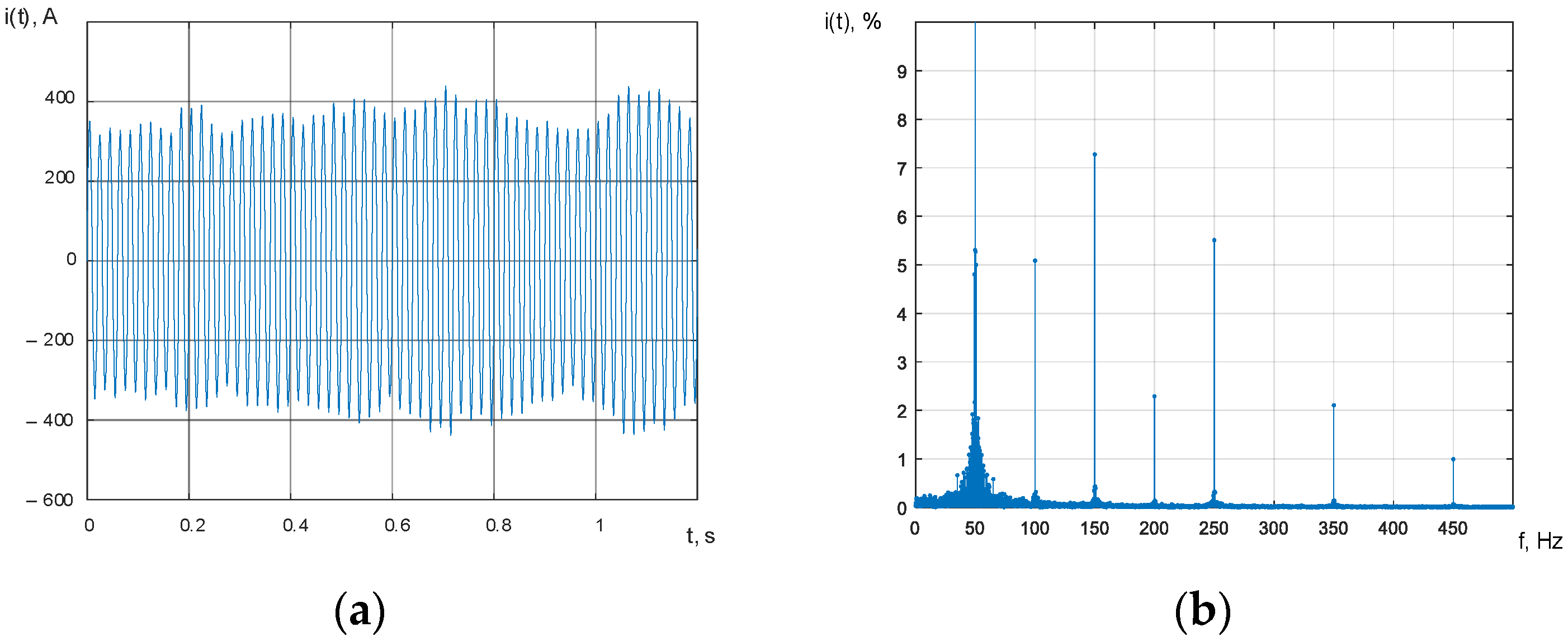
As an example, Figure 2a shows one of the implementations of the current curve of phase A of the arc furnace for melting EAF-100 steel, which is an amplitude-modulated oscillation in accordance with the expression (13). The modulating random process $\xi (t)$ is given by an exponential autocorrelation function (15), where the variance of the current oscillations is $D_{\xi }=9331.2 {\mathrm{A}}^2$. Figure 2b shows the corresponding frequency spectrum of the phase A network current curve of the EAF-100 furnace, obtained using a fast Fourier transform directly from the simulated current curve. Figure 3a shows one of the implementations of the current curve of phase A of the EAF-100 furnace, which is an amplitude-modulated oscillation, where the random modulation process $\xi (t)$ is determined by an exponential-cosine autocorrelation function of the form (16) with the parameters: $D_{\xi }=9331.2 {\mathrm{A}}^2$, $\alpha =1.47 {\mathrm{s}}^{-1}$, and ${\omega }_0=2.69 {\mathrm{s}}^{-1}$. Figure 3b shows the corresponding amplitude spectrum. Figure 4a shows the implementation of the phase A current curve of the EAF-100 furnace, which is an amplitude-modulated oscillation, where the random modulation process $\xi (t)$ is determined by the exponential-cosine-sine autocorrelation function of the form (17), with the same parameters as in the case of the exponential-cosine autocorrelation function. Figure 4b shows the corresponding amplitude spectrum.

As a result of numerous studies, it was found that for the given parameters of the random process, the expected value of the current curve distortion coefficient $E\left[K_I\right]$ is

• $E\left[K_I\right]=15.7\%$, when using the exponential autocorrelation function;
• $E\left[K_I\right]=17.3\%$, when using the exponential-cosine autocorrelation function;
• $E\left[K_I\right]=15.6\%$, when using the exponential-cosine-sine autocorrelation function.

Therefore, the error in estimating the current curve distortion factor when using different types of autocorrelation functions to simulate the same random process of changing the arc furnace load current did not exceed 10%. This result allows us to conclude that when conducting various tests simulating the random process of changing the load current of an arc furnace, it is possible to use any type of autocorrelation function (15)–(17), depending on the scope of the problems being solved.

When examining the problem of electromagnetic compatibility during the operation of arc furnaces for steel melting by modeling random processes of changes in load currents, one type of autocorrelation function was replaced by another based on the equality of areas under the autocorrelation function curves.

In general, such an approach is in principle unacceptable. This is due to the fact that the factor determining the value of the distortion coefficient of the current waveform is not the energy of the random process of changing load current, but its speed of change, which is characterized by the parameters of the autocorrelation function. The test results have shown that as the damping coefficient α of the angular frequency of the autocorrelation function ω₀ increases, the distortion coefficient of the current curve also increases. In such a case, replacing the exponential-cosine autocorrelation function in the form (15) with an exponential function in the form (14) and determining the equivalent damping coefficient α_e using the expression (18) may lead to an overestimation of the value of the distortion coefficient of the current curve.

5. Calculation of Compensating Device Parameters for the Random Nature of Electrical Loads

Let us consider the electrical system shown in Figure 1 for the case without reactive power compensation. The RMS value of the voltage at the point of connection of the variable load is defined as the difference between the network voltage and the voltage drop across the network impedance:

$$U_o=U_s-I_s{X}_s\mathrm{s}\mathrm{i}\mathrm{n}\phi ,$$

(19)

where φ is the load phase shift angle, and I_s is the RMS value of the network current, which in the absence of compensation is equal to the load current determined similarly to the instantaneous waveform (13):

$$I_s=I_o=\left(\xi (t)+1\right)I,$$

(20)

Then, the RMS value of the voltage on the load is

$$U_o=U_s-\left(\xi (t)+1\right)I{X}_s\sin \phi =U_s-I{X}_s\sin \phi -\xi (t)I{X}_s\sin \phi .$$

(21)

In expression (21), the difference between the first two components is the effective value of the voltage at the point of load connection, without taking into account the random process modulation of the current waveform, while the network reactance can be determined as

$$X_s=\frac{U^2}{S_k^{″}},$$

(22)

where $S_k^{″}$ is the short-circuit power of the network.

Then, taking into account relation (6), we obtain

$$U_o=U-\xi (t)I\frac{U^2}{S_k^{″}}\sin \phi =\left(1-\xi (t)\frac{Q_o}{S_k^{″}}\right)U,$$

(23)

where Q_o is the reactive power of the load.

Moving to instantaneous voltage values, an expression can be written for the voltage at the load connection point, taking into account the modulation ξ(t) of the load current curve:

$$u_o(t)=\left(1-\xi (t)\frac{Q_o}{S_k^{″}}\right)u(t)=\left(1-a\xi (t)\right)u(t),$$

(24)

where $a=Q_o/S_k^{″}$.

Let us consider the issue of reactive power compensation for the case when a compensating device in the form of a capacitor bank is connected in parallel with a nonlinear fast-changing load (Figure 1).

As in the case of reactive power compensation in a network with higher harmonics, it is necessary to meet condition (7), in which the network current is equal to

$$i_s(t)=i_o(t)+i_k(t),$$

(25)

where i_k(t) is the current flowing through a capacitor bank with capacity C,

$$i_k(t)=C\frac{du(t)}{dt}=C\frac{d\left(1-a\xi (t)\right)u(t)}{dt}=C\left[\left(1-a\xi (t)\right)u\prime (t)-a\xi \prime (t)u(t)\right],$$

(26)

wherein

$$\xi \prime (t)=\frac{d\xi (t)}{dt}.$$

(27)

Taking into account expressions (13), (25) and (26) we obtain

$$i_s(t)=\left(\xi (t)+1\right)i(t)+C\left[\left(1-a\xi (t)\right)u\prime (t)-a\xi \prime (t)u(t)\right]$$

(28)

The square of the RMS value of the current in the supply network is

$$I_s^2=\frac{1}{T}{\displaystyle \underset{0}{\overset{T}{\int }}{\left[\xi (t)+1\right]}^2}{\left[i(t)\right]}^{2}dt+\frac{1}{T}{\displaystyle \underset{0}{\overset{T}{\int }}2C \left[\xi (t)+1\right]} i(t)\left\{\left[1-a\xi (t)\right] u\prime (t)-a\xi \prime (t)u(t)\right\}dt+\frac{1}{T}{\displaystyle \underset{0}{\overset{T}{\int }}{C}^2}{\left\{\left[1-a\xi (t)\right] u\prime (t)-a\xi \prime (t)u(t)\right\}}^{2}dt$$

(29)

and the derivative of the square of the current with respect to the capacitance C takes the following form:

$$\frac{d{I}_s^2}{dC}=\frac{2}{T}{\displaystyle \underset{0}{\overset{T}{\int }}\left[\xi (t)+1\right]} i(t)\left\{\left[1-a\xi (t)\right] u\prime (t)-a\xi \prime (t)u(t)\right\}dt+\frac{2C}{T}{\displaystyle \underset{0}{\overset{T}{\int }}{\left\{\left[1-a\xi (t)\right] u\prime (t)-a\xi \prime (t)u(t)\right\}}^{2}dt} .$$

(30)

By equating the derivative $\frac{d{I}_s^2}{dC}$ to zero, we can determine the capacity C and then the power of the capacitor bank:

$$Q_k=U_N^2\omega C=U_N^2\omega \frac{{\displaystyle \underset{0}{\overset{T}{\int }}\left(\xi \left(t\right)+1\right)}\left(i\left(t\right)\right)\left[\left(1-a\xi \left(t\right)\right)u\prime \left(t\right)-a\xi \prime \left(t\right)u\left(t\right)\right]dt}{{\displaystyle \underset{0}{\overset{T}{\int }}{\left[\left(1-a\xi \left(t\right)\right)u\prime \left(t\right)-a\xi \prime \left(t\right)u\left(t\right)\right]}^2}dt},$$

(31)

where U_N is the rated voltage of the capacitor bank.

The expected value of the capacitor bank power can be determined using the random process linearization method:

$$E{Q}_k=U_N^2\omega \frac{{\displaystyle \underset{0}{\overset{T}{\int }}E\left[\left(\xi \left(t\right)+1\right)\left(u\prime \left(t\right)-a\xi \left(t\right)u\prime \left(t\right)-a\xi \prime \left(t\right)u\left(t\right)\right)\right]i\left(t\right)}dt}{{\displaystyle \underset{0}{\overset{T}{\int }}E{\left[\left(u\prime \left(t\right)-a\xi \left(t\right)u\prime \left(t\right)-a\xi \prime \left(t\right)u\left(t\right)\right)\right]}^2}dt}.$$

(32)

Taking into consideration that the expected values of the random processes ξ(t) and ξ′(t) are equal to zero (E[ξ(t)] = 0 and E[ξ′(t)] = 0) and that the coefficient of their mutual autocorrelation $K_{\xi {\xi }^{\prime }}=0$, we get

$$E{Q}_k=\frac{U_N^2\omega \left(1-a{D}_{\xi }\right){\displaystyle \underset{0}{\overset{T}{\int }}i\left(t\right)u\prime \left(t\right)}dt}{\left(1+a^2{D}_{\xi }\right){\displaystyle \underset{0}{\overset{T}{\int }}{u\prime \left(t\right)}^2}dt+\frac{a^2{D}_{\xi \prime }}{{\omega }^2}{\displaystyle \underset{0}{\overset{T}{\int }}{u\left(t\right)}^2}dt},$$

(33)

where D_ξ is the variance of the centered stationary random process ξ(t), and D_ξ′ is the variance of the derivative of this process.

Substituting into this expression the expansion of current and voltage into the Fourier series (3) and (4), we obtain:

$$E{Q}_k=\frac{U_N^2\left(1-a{D}_{\xi }\right){\displaystyle \sum _{h=1}^{\infty }h{U}_h{I}_h\sin {\phi }_h}}{\left(1+a^2{D}_{\xi }\right){\displaystyle \sum _{h=1}^{\infty }{h}^2{U}_h^2}+\frac{a^2{D}_{\xi \prime }}{{\omega }^2}{\displaystyle \sum _{h=1}^{\infty }{U}_h^2}}.$$

(34)

The requirement for the differentiation of the random process ξ(t) is the continuity of the derivative of its autocorrelation function around the point τ = 0. This requirement is met by the exponential-cosine-sine autocorrelation function in the following form:

$$K_{\xi }\left(\tau \right)=D_{\xi }{e}^{-\alpha \left|\tau \right|}\left(\cos {\omega }_0\tau +\frac{\alpha }{{\omega }_0}\sin {\omega }_0\left|\tau \right|\right),$$

(35)

and hence the variance of the derivative of the process ξ(t):

$$D_{\xi \prime }={\left.-\frac{d^2{K}_{\xi }\left(\tau \right)}{d{\tau }^2}\right|}_{\tau =0}={\left.D_{\xi }\left({\alpha }^2+{\omega }_0^2\right)e^{-\alpha \left|\tau \right|}\left(\cos {\omega }_0\tau +\frac{\alpha }{{\omega }_0}\sin {\omega }_0\left|\tau \right|\right)\right|}_{\tau =0}=D_{\xi }\left({\alpha }^2+{\omega }_0^2\right)$$

(36)

Substituting expression (36) into Equation (34), we obtain

$$E{Q}_k=\frac{U_N^2\left(1-a{D}_{\xi }\right){\displaystyle \sum _{h=1}^{\infty }h{U}_h{I}_h\sin {\phi }_h}}{\left(1+a^2{D}_{\xi }\right){\displaystyle \sum _{h=1}^{\infty }{h}^2{U}_h^2}+\frac{a^2{D}_{\xi }({\alpha }^2+{\omega }_0^2)}{{\omega }^2}{\displaystyle \sum _{h=1}^{\infty }{U}_h^2}}.$$

(37)

6. Calculation Results

Let us consider an example of calculating the power of the capacitor bank needed to compensate for reactive power during the operation of a steel arc furnace EAF-100 with the following parameters: rated power of the transformer S_NT = 45 MV·A, rated voltage of the primary winding of the transformer U_N = 35 kV, rated current of the furnace I_N = 400 A. Let us consider three cases.

6.1. Calculation of Capacitor Bank Power Based on the Fundamental Harmonic of Current and Voltage

In this case, we use the furnace ratings as the RMS values of the fundamental harmonics of current and voltage. The value of the phase angle was determined experimentally and was φ₁ = 26°. Then, the capacity of the capacitor bank can be defined as

$$Q_k=U_1{I}_1\sin {\phi }_1=35\cdot 0.4\cdot \sin {26}^{\circ }=6.137 \mathrm{Mvar}.$$

(38)

6.2. Calculation of the Power of Capacitor Banks Taking into Account Higher Harmonics

Table 1. Parameters of higher harmonics of current and voltage measured during the operation of the arc furnace EAF-100.

Parameter	Harmonic Number of Order h
	2	3	4	5	6	7	8	9
Ih/I1, %	5.1	7.2	2.3	5.5	0	2.1	0	1.0
Uh/U1, %	2.5	3.6	1.2	3.0	0	1.0	0	0.5
φh, °	87	−89	52	−55	0	98	0	−90

contains the relative values of higher harmonics of current and voltage and the corresponding phase angles obtained experimentally on the basis of the measurements made during the operation of the EAF-100 arc furnace in question at one of the metallurgical enterprises (Mariupol, Ukraine). The measurements were performed using the Power Quality analyzer Fluke 435.

To calculate the power of the compensating device, taking into account higher harmonics, the source of which is the EAF-100 arc furnace, we use the expression (12). As a result of the calculations, we get

Q_k = 5.734 Mvar.

(39)

6.3. Calculation of the Power of Capacitor Banks Taking into Account Higher Harmonics and Interharmonics

In this case, it is necessary to estimate the expected value of the capacitor bank capacity according to Equation (35). Let us assume that in order to take into account interharmonics, the EAF-100 current curve is modulated by a random process with an exponential-cosine autocorrelation function with the following parameters: oscillation current variance D_ξ = 9331.2 A², damping factor of the autocorrelation function α = 1.47 s⁻¹, angular frequency ω₀ s⁻¹. The parameters of the autocorrelation function of the modulating random process were obtained experimentally using measurement data for the melting phase of the EAF-100 arc furnace.

Then, as a result of calculations according to relation (31), we obtain

EQ_k = 5.71 Mvar.

(40)

For most practical cases $0<a<0.2$; $0<D_{\xi }<{(0.5)}^2=0.25$; $\alpha <<\omega , {\omega }_0<<\omega$, so expression (38) can be simplified to

$$E{Q}_k=\left(1-a{D}_{\xi }\right)U_N^2\frac{{\displaystyle \sum _{h=1}^{\infty }h{U}_h{I}_h\sin {\phi }_h}}{{\displaystyle \sum _{h=1}^{\infty }{h}^2{U}_h^2}}.$$

(41)

The comparison of Equations (12), (38) and (41) shows directly that in order to minimize energy losses in the power supply network, the load variability should be taken into account in the process of selecting the power of reactive power compensation devices. In the case considered in this study, when the compensator is a capacitor bank, its power will be lower when taking into account the rapidly changing nature of the load.

7. Conclusions

The research conducted shows that in power networks supplying rapidly changing nonlinear loads causing an occurrence of interharmonics in current and voltage waveforms, a power correction of reactive power compensating devices is required.

When examining non-sinusoidal conditions in electrical networks with rapidly changing nonlinear loads, the non-sinusoidal current curve can be represented as an amplitude modulated waveform with randomly varying amplitude and initial phase.

The use of a centered stationary random process with a given autocorrelation function as a modulating signal allows us to obtain analytical expressions for calculating the probabilistic current characteristics of fast-varying loads and parameters of reactive power compensating devices.

When solving problems related to both the phenomenon of the heating of wires and parts of electrical devices carrying current during the flow of non-sinusoidal current, as well as the assessment of electromagnetic compatibility parameters during the operation of rapidly changing nonlinear loads, the autocorrelation function of a modulating random process can be represented by any of the three types according to expressions (15)–(17).

In the study of processes related to the heating of wires and current-carrying parts of electrical devices and energy losses, it is possible to replace one type of autocorrelation function modulating a random process with another; however, when examining the problem of electromagnetic compatibility, such an exchange turns out to be unacceptable. When solving problems related to reactive power compensation in electrical networks with rapidly changing nonlinear loads, the autocorrelation function of the modulating random process must have a continuous derivative around the point $\tau =0$ to ensure the condition of differentiability of the random process. This requirement corresponds to the autocorrelation function in expression (17).

If a capacitor bank is used as a compensation device, its power, determined by the condition of minimal energy losses in the power supply network, should be lower than without, taking into consideration the rapidly changing nature of the load and interharmonics.

In the calculation example presented herein, taking into account higher harmonics and interharmonics in the voltage and current waveforms of unsettled receivers, the power of the capacitor bank was reduced by approximately 7%, which allows for reduced investment costs. An additional effect is the reduction of energy losses in the power supply network, estimated at 3–5%.

This study is the first step in solving the problem of reactive power compensation in electrical networks containing interharmonics. The analysis concerns the use of capacitor banks as compensating devices for reactive power in rapidly changing loads, such as arc furnaces and welding equipment.

The authors plan further research in two directions: The first direction is the use of passive filter-compensating devices, active filters, and STATCOM compensators to compensate the reactive power of fast-varying loads and to improve power quality.

The second direction results from the fact that the sources of interharmonics are also various types of power electronic converters, especially frequency converters used in speed-controlled drive systems. The completely different nature of interharmonic generation in such loads requires a different approach to the methods for calculating and compensating reactive power.