A Stochastic Multi-Objective Model for China’s Provincial Generation-Mix Planning: Considering Variable Renewable and Transmission Capacity

Abstract

The uncertain output of variable renewables adds significant challenges to the generation of affordable, reliable, and sustainable power sources in a country or region. Therefore, we propose a new stochastic nonlinear multi-objective model to optimize the power generation structure in 31 provinces of China. Considering variable renewable integration, we use Monte Carlo simulation to describe the randomness and uncertainty of renewable power output. The learning curve in the exponential expression is used to describe the nonlinear relationship between generation cost and installed capacity. The optimized results show that China can substitute fossil power with clean power. Renewable power will account for more than 42% of total power in the optimal power generation structure in 2040. In particular, the annual average growth rate of non-hydro renewable generation is expected to be 12.06%, with solar photovoltaic (PV) power growing the most by 17.95%. The share of renewable power exceeds that of thermal power in 14 provinces, and PV power represents the highest proportion at 30.21%. Reducing transmission capacity can promote the development of advantageous power in each region, such as wind power in the Northwest region and PV power in the South region, with the share increasing by 36.33% and 132.59%, respectively.

1. Introduction

Ongoing socio-economic development ensures persistent growth in global power demand. In 2018, global power demand reached 23,000 TWh with annual growth of 4%, almost twice that of energy demand [1]. Increased power generation is critical to meet the dramatic growth in demand and ensure the security of the power supply. Various sources of power generation (thermal power, nuclear power, and renewable power) have different outputs per unit of installed capacity, costs, and impacts. This calls for an optimal power generation mix that is cost-effective and low-emission, with sufficient energy capacity [2]; that is, an optimized combination of various power generation sources. The influence of seasonal changes, diurnal variations, and geographical differences create intermittent and uncertain renewable energy generation hours and power output [3]. These uncertainties inevitably increase the amount of reserves and reduce the efficient operation of thermal power plants and the replacement of thermal electricity generation by Intermittent Renewable Energy Sources [4].

In addition, future changes in renewable unit power generation costs are a significant factor affecting power generation-mix planning. The unit generation cost of renewable energy is typically reflected in the learning rate of the cost curve, which is a nonlinear relationship with cumulative installed capacity [5]. The cost estimation error could be significant in a linear model with exogenous power generation costs. Such costs cannot be modified during model solving, which means that there is a development barrier to renewable power in the initial settings. On the contrary, the endogenous costs with a learning curve for technology changes in a nonlinear model are more realistic. Such a model can significantly reduce uncertainty and improve the robustness of the solution [6]. In addition, the learning effect is a key driving mechanism behind the cost reduction of wind and solar power [7]. The dynamic change of the cost in model solving can truly reflect the technological development level of renewable energy to realize the accurate estimation of the cost of renewable energy generation.

Power generation-mix planning aims to build a power generation portfolio plan that optimizes a specific target—power generation cost, for example—while satisfying certain constraints, such as power demand, resource potential, and environmental protection. Early studies on power generation-mix optimization focused on minimizing costs [8,9] or maximizing net present value [10]. Such single-objective models are effective for small power systems, but they are inefficient for complex systems that involve multiple targets, standards, and stakeholders [11]. On the contrary, a multi-objective model can consider the various interest concerns of different stakeholders, providing a wide range of alternatives through trade-offs for better support in generation-mix optimization. This optimization introduces multiple objectives that exacerbate the conflicts inherent in optimization [12]. Al Shidhani et al., proposed a multi-objective optimization model integrating four objective functions, including minimization of total discounted costs, carbon emissions, land use, and social opposition to determine Indonesia’s most suitable electricity generation mix [13]. By trade-offs between the system costs and the life cycle greenhouse gas emissions of power systems, Junne et al., determined the structure of the power plant portfolio in Europe and North Africa [14]. Similar multi-objective optimization models can be found in Makhloufi et al., for Algeria [15], Luz et al., for Brazil [16], and Atabaki and Aryanpur for Iran [12].

These studies focused on expressing the objectives and constraints in a linear formulation. However, with high levels of renewable energy power penetration, power supply uncertainty increases, making the relationship between factors such as generation cost, penetration of renewable power, and decision variables (e.g., power generation) far from a simple linear relationship. The existing deterministic linear optimization model [14,15,16] does not apply to the power generation-mix planning problem, which has uncertainty and nonlinearity due to the large-scale penetration of renewable power. Therefore, some studies have established nonlinear multi-objective optimization models by the nonlinear expression of installed capacity [17] or the nonlinear relationship between installed capacity and the levelized cost of electricity [18]. However, such models cannot deal with the uncertainty and intermittent renewable power caused by meteorological conditions. A random sampling method, Monte Carlo simulation (MCS), is widely used to describe this type of uncertainty. In [19], MCS was utilized to describe uncertainty at a random hour for each scenario. The detailed variability at the 5 min level in solar generation was expressed by MCS in [20]. These simulation studies described the uncertainty of variable renewable power output at intervals of hours or minutes, which cannot describe the output uncertainty in terms of the years involved in mid- to long-term planning. Therefore, for medium- and long-term generation-mix planning, describing the annual output uncertainty of renewable power is the first research gap that we address.

Second, the power supply and demand constraints are simplified to a balance of total generation and demand without considering interregional power transmission in existing power structure optimization. However, it is impossible to determine the composition of each region in the total amount without considering power transmission, especially for a country with a vast area such as China. This gap may lead to limited support for the optimization results in decision-making. Wang et al., study only considered the unchanged transmission capacity of ultra-high-voltage lines between regions every ten years, ignoring the transmission capacity of existing high and extra-high voltage lines [21]. A similar single-objective model proposed by Hui et al., has another drawback, as the transmission capacity remains unchanged during the whole planning period [22]. Chen et al., ignored future changes in transmission capacity [23]. In these cases, the optimization results were quite different from the actual future developments, implying limited decision-making support. Therefore, the second research gap is how to determine the impact of transmission capacity on the power generation structure of each province by combining the existing and planned transmission capacities.

Third, regarding the scope of optimization, the aforementioned models mainly focused on the country as a whole [12,15,17] or on one region [21,22,23]. The former approach cannot reasonably provide information on implementing the results in various regions and provinces. The actual feasibility of the results is difficult to guarantee. The latter approach ignores the connection with other regions and cannot include the impact of other regions on local power supply and demand, which can lead to an unreasonable generation mix. Especially in China, there are many differences between provinces regarding economic development levels, power demands, resource endowments, etc. Therefore, the third research gap is how to consider different Chinese provinces’ resource potentials, power demands, and environmental responsibilities to achieve the optimal power generation mix of each province.

Fourth, the existing multi-objective model often utilizes specific solution strategies to transform multi-objective models into single-objective models, and only a unique solution can be obtained [12,14,17]. The single-objective model must be solved repeatedly to generate Pareto optimal solutions, making the decision information fuzzy because the results are often inconsistent among the independent optimization processes [24]. On the contrary, multi-objective evolutionary algorithms, such as the elitist non-dominated sorting genetic algorithm (NSGA-II), the non-dominated sorting particle swarm optimization (NSPSO), and the strength Pareto evolutionary algorithm-II (SPEA-II), can deal with multi-objective problems more effectively by obtaining a set of independent non-dominated Pareto optimal solutions in a single run [25]. Thus, obtaining the optimal generation mix by compromising contradictory goals and providing a more comprehensive decision-making reference comprise the fourth gap we deal with.

Therefore, considering the high penetration level of renewable power, we propose a stochastic nonlinear multi-objective optimization (SNM) model to obtain China’s optimal power generation structure at the province level. The main contributions of this paper are as follows: (a) Nonlinear formulation is used to describe the variation of the levelized cost of electricity (LCOE) with technological progress, instead of a fixed cost as in existing studies [13,16], which ignored the dynamic cost that comes with technological progress. Monte Carlo simulation simulates the uncertainty of renewable energy output at yearly intervals instead of by the hour [19] or minute [20], providing robust results for medium- and long-term power generation planning; (b) Interregional power transmission capability is an important constraint in the model. It can avoid mismatching between planned power generation capability and transmission capability, leading to extensive power curtailment in China; (c) The intelligent algorithm NSPSO is used to obtain Pareto solutions by conducting a trade-off between contradicting objectives, instead of the objectives weighted sum method. Four representative solutions are selected from the optimal Pareto front according to decision makers’ objective preferences, providing comprehensive decision support under different preferences; (d) We obtain the complete 31 provinces’ cumulative installed capacity roadmap for six types of power generation sources (thermal, nuclear, hydro, wind, solar PV, and biomass) in China from 2017 to 2040, rather than that for the whole of China [17] or for a single region [23]. The detailed roadmap can provide a feasible plan and a valuable reference for the installation planning of both provinces and the country.

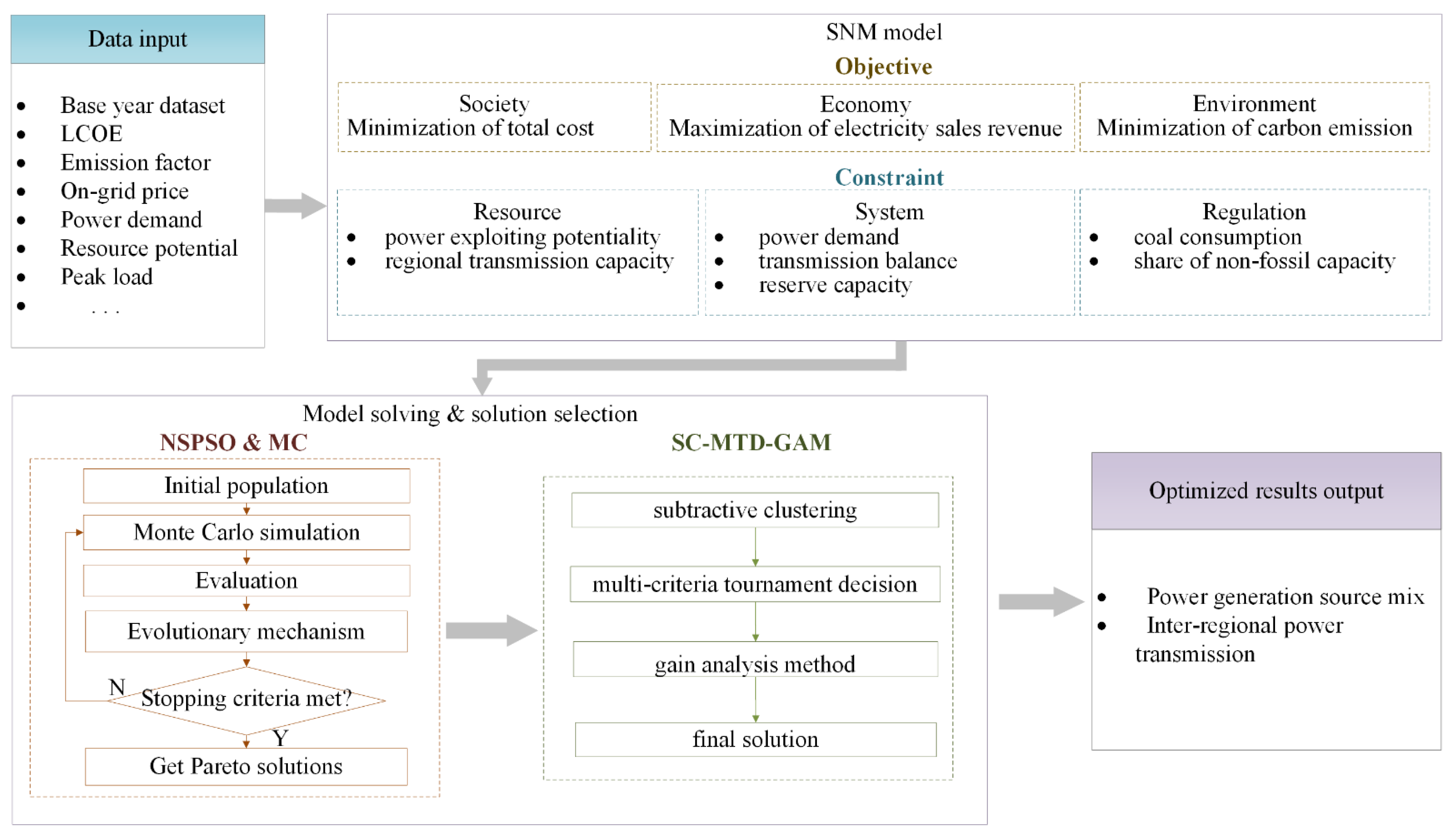
2. The Proposed Power Source Optimization Model

2.1. Assumptions

We propose the following assumptions for a stochastic nonlinear multi-objective model for optimizing province-level power generation structures in China.

(a)

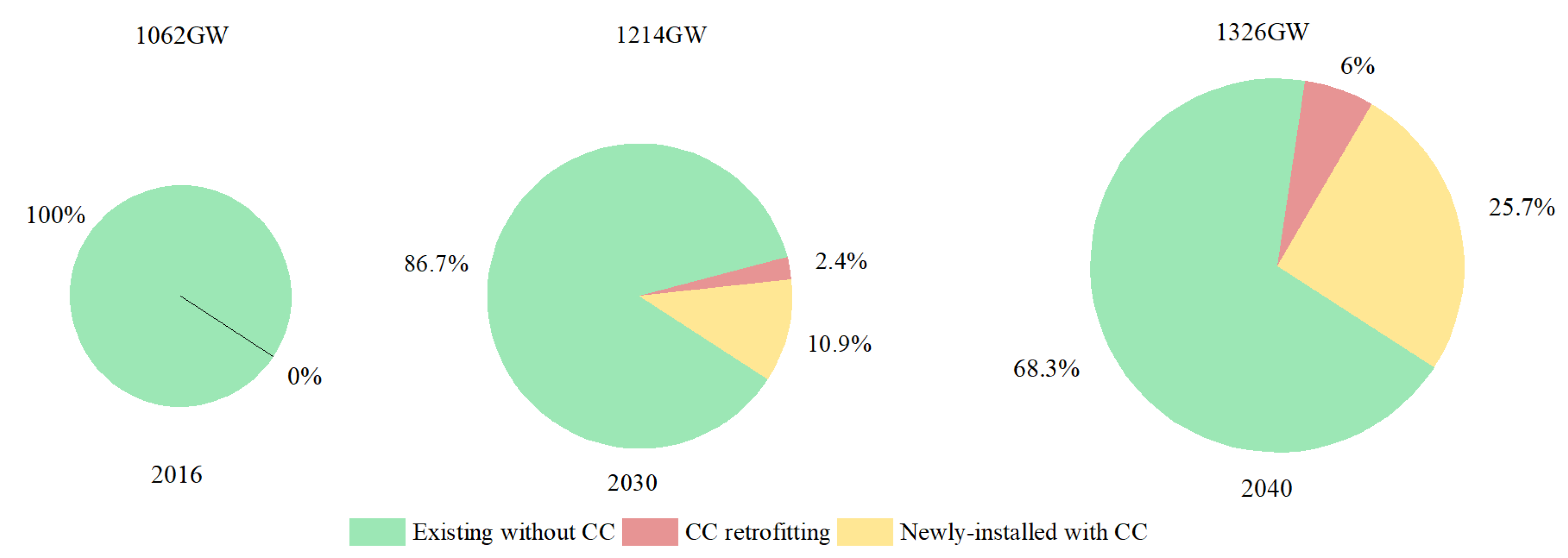
Existing thermal power units will start carbon capture (CC) retrofitting in 2025. At the same time, newly installed thermal power units must be equipped with carbon capture equipment. CC retrofitting only considers the additive carbon capture equipment, while the subsequent carbon storage equipment is not included.

(b)

We divide China’s transmission network into six regions, as listed in Appendix A,

Table A1. Regional division.

Power Grid	Provinces, Municipalities or Autonomous Regions
Northeast (NE)	Liaoning, Jilin, Heilongjiang, Inner Mongolia
North (N)	Beijing, Tianjin, Hebei, Shanxi, Shandong
East (E)	Shanghai, Jiangsu, Zhejiang, Anhui, Fujian
Central (C)	Henan, Hubei, Hunan, Jiangxi, Chongqing, Sichuan
South (S)	Yunnan, Guizhou, Guangxi, Guangdong, Hainan
Northwest (NW)	Shaanxi, Gansu, Qinghai, Ningxia, Tibet, Xinjiang

. The provinces’ power transmission in the regions is not considered, due to a lack of available data.

(c)

With a focus on the optimal power generation mix, renewable energy resources are assumed to be used only for electricity generation, so other usage patterns, such as heat storage, hydrogen, and underground energy storage, are not considered.

2.2. Objective Functions

(a)

Minimization of the Total Cost

Achieving the lowest cost is a primary goal of economic activities. To reflect the costs of different power sources more comprehensively, together with the power generation transmission costs, we include the environmental costs of power generation processes. The environmental costs include carbon emissions and non-carbon external costs, such as the external costs of the effect of electricity production on human health, crop yields, biodiversity, and material damage. The total cost is expressed by Equation (1).

$$\min F1={\displaystyle \sum _{t\in T}((E({\displaystyle \sum _{i\in I}{\displaystyle \sum _{j\in J}(Q_{i,j,t}{h}_{i,j,t}{c}_{j,t}+Q_{i,j,t}{h}_{i,j,t}{s}_{j,t}+Q_{i,j,t}{h}_{i,j,t}e{l}_j{o}_t)}})+{\displaystyle \sum _{i\in I}{\displaystyle \sum _{j\in J}{I}_{i,t}{u}_{i,t}}})/{(1+r)}^t)}$$

(1)

where for power generation source $j$ in province $i$ at year $t$, $Q_{i,j,t}{h}_{i,j,t}{c}_{j,t}$ is the generation costs, $Q_{i,j,t}{h}_{i,j,t}{s}_{j,t}$ is the non-carbon external costs, $Q_{i,j,t}{h}_{i,j,t}e{l}_j{o}_t$ represents the carbon emissions costs, and $I_{i,t}{u}_{i,t}$ represents the power transmission costs.

For the cost of CC retrofitting, we only consider the additive carbon capture equipment to reduce carbon emissions. In contrast, the costs in the subsequent carbon transportation and carbon storage processes are not included. Therefore, CC retrofitting is also considered as a power generation source in the proposed model, but it differs from existing thermal power units in the cost input and performance parameters. The details are incorporated into Equations (2) and (3).

$$Q_{i,1,t}=\{\begin{array}{l}{Q}_{i,1,t-1}{(1-{\eta }_{i,1,t-1})}^t+X_{i,1,t}i\in I;t\in \left\{1,2,...,9\right\}\\ Q_{i,1,t-1}{(1-{\eta }_{i,1,t-1})}^t-X_{i,2,t}i\in I;t\in \left\{9,10,...,\left|T\right|\right\}\end{array}$$

(2)

$$Q_{i,2,t}=\{\begin{array}{l}0i\in I;t\in \left\{1,2,...,9\right\}\\ Q_{i,2,t-1}+X_{i,1,t}+X_{i,2,t}i\in I;t\in \left\{9,10,...,\left|T\right|\right\}\end{array}$$

(3)

$$Q_{i,j,t}=Q_{i,j,t-1}+X_{i,j,t}-Q_{i,j,t-L{T}_j+1}j\in \left\{3,...,\left|J\right|\right\};i\in I;t\in T$$

(4)

where for province $i$ at year $t$, $Q_{i,1,t-1}{(1-{\eta }_{i,1,t-1})}^t$ is the cumulative installed service capacity of existing thermal power, $Q_{i,2,t-1}+X_{i,1,t}+X_{i,2,t}$ is the installed capacity of thermal power with CC equipment since 2025, including newly installed thermal power units with CC equipment and the retrofitting capacity of existing thermal power units, and $Q_{i,j,t-1}+X_{i,j,t}-Q_{i,j,t-L{T}_j+1}$ represents the cumulative installed service capacity of power generation source $j$ in year $t$, which equals the cumulative installed capacity in year $t-1$ plus the newly installed capacity in year $t$ minus the decommissioned capacity in year t under the technical lifetime ($L{T}_j$).

Existing studies showed that the process evaluation of the power generation technology follows the mechanism of the learning curve [26]. Thus, the related costs could gradually decrease as the technology matures. Therefore, the levelized cost of each power generation source is assumed to follow the learning curve as in Equation (5) to reflect the learning effect of technology development [27]. In addition, the evaluation process of CC technology conforms to the learning curve, and due to the small scale in the base year, its cost follows another learning curve as in Equation (7) [28].

$$c_{j,t}=c_{j,t_0}{({\displaystyle \sum _{i\in I}{Q}_{i,j,t}}/{\displaystyle \sum _{i\in I}{Q}_{i,j,t_0}})}^{-b_n{}^j}j\in J;t\in T$$

(5)

$$l{r}_j=1-2^{-b_n{}^j}$$

(6)

$$c_{2,t}=c_{2,t_0}{e}^{-\theta t}$$

(7)

The net generation output will inevitably shrink due to significant energy loss when the existing coal-fired units are retrofitted with CC. Therefore, the generation cost per unit with the CC device should be $G{C}_t={\displaystyle \sum _{i=1}^I\lambda Q_{i,2,t}{h}_{i,2,t}{c}_{j,t}}$ the capacity-shrinking coefficient representing the proportion of the reduced generation by the per unit installed capacity of the thermal power unit after CC retrofitting. Similarly, each expression in the following text only calculates power generation; the coefficient $\lambda$ needs to be multiplied before $Q_{i,2,t}$.

(b)

Maximizing total electricity sales revenue of power generation enterprises

Power generation structure optimization at the regional level must consider local economic benefits measured by the electricity sales revenue of power generation enterprises, as in Equation (8).

$$\max F2={\displaystyle \sum _{t\in T}(E({\displaystyle \sum _{i\in I}{\displaystyle \sum _{j\in J}{Q}_{i,j,t}{h}_{i,j,t}{a}_{i,j,t}}})/{(1+r)}^t)}$$

(8)

where $Q_{i,j,t}{H}_{i,j,t}{a}_{i,j,t}$ represents the electricity sales revenue of power generation source $j$ of power generation enterprises in province $i$ in year $t$.

(c)

Minimization of carbon emissions

The transformation of the power generation structure from carbon-intensive to low carbon is an important measure for global climate change. In 2016, the power sector accounted for 48.1% of total carbon emissions in China [29]. Therefore, minimum carbon emissions from the power sector are an important step for China to achieve its carbon emissions targets. Although renewable energy does not produce carbon emissions directly in the power generation process, carbon emissions are still present in the production and manufacturing process of power generation. To reasonably reflect carbon emissions among various power sources, we use the life cycle analysis method to measure the carbon emissions generated per power generation unit.

$$\min F3=E({\displaystyle \sum _{t\in T}{\displaystyle \sum _{i\in I}{\displaystyle \sum _{j\in J}{Q}_{i,j,t}{h}_{i,j,t}e{l}_j}}})$$

(9)

where $Q_{i,j,t}{h}_{i,j,t}$ is generated by the power generation source $j$ in the province and $e{l}_j$ represents the life cycle carbon emission factor per unit of power generation of power source $j$.

2.3. Constraints

(a)

Regional power demand constraint

The premise of power generation structure optimization is that power generation must meet the power demand from economical production and residents’ daily needs. At the province level, the available power of a province cannot be less than its electricity demand. The power generation can be considered as its power generation $Q_{i,j,t}{h}_{i,j,t}$ plus transmitted-in power $I_{i,t}$ from other provinces minus transmitted-out power $O_{i,t}$ to other provinces.

$${\displaystyle \sum _{i\in k}(E({\displaystyle \sum _{j\in J}{Q}_{i,j,t}{h}_{i,j,t}})-O_{i,t}+I_{i,t})(1+l_{i,t})}\ge {\displaystyle \sum _{i\in k}{D}_{i,t}}k\in K;t\in T$$

(10)

Power demand can be reasonably estimated based on the province’s GDP growth rate ${\gamma }_{i,t}$, as in Equation (11).

$$D_{i,t}=b_{i,t}\cdot gd{p}_{i,t0}\cdot (1+{\gamma }_{i,t})$$

(11)

Power supply aims to balance supply and demand ability without power surplus or shortage. Excess power generation is often used to ensure the stability of power quality to meet production and living needs because a power shortage will cause higher economic costs and social losses than a power surplus. Therefore, a power surplus should be minimized to reduce economic costs and resource waste. Introducing a positive deviation variable in Equation (10) converts the unequal constraints into an equation form. It then minimizes the positive deviation variable as the optimization goal to achieve the minimum power surplus. The transformed constraints and corresponding goals are as follows:

$${\displaystyle \sum _{i\in k}(E({\displaystyle \sum _{j\in J}{Q}_{i,j,t}{h}_{i,j,t}})-O_{i,t}+I_{i,t})(1+l_{i,t})}-d_{k,t}^{+}={\displaystyle \sum _{i\in k}{D}_{i,t}}$$

(12)

$$\min d={\displaystyle \sum _{t\in T}{\displaystyle \sum _{\mathrm{k}\in K}{d}_{k,t}^{+}}}$$

(13)

where $d_{k,t}^{+}$ is the deviation variable representing the power surplus of electricity supply exceeding the electricity demand in region $k$ in year $t$. Therefore, power demand constraints are finally transformed into the following objectives:

$$\min d(X)={\displaystyle \sum _{i\in k}(E({\displaystyle \sum _{j\in J}{Q}_{i,j,t}{h}_{i,j,t}})-O_{i,t}+I_{i,t})(1+l_{i,t})}-{\displaystyle \sum _{i\in k}{D}_{i,t}}$$

(14)

(b)

Reliability of the power supply constraint

To meet regional power demand, reserve capacity must be considered to ensure power supply reliability with sufficient output capacity [30]. Reserve capacity is divided into load reserve, accident reserve, and maintenance reserve. The security of the regional power supply must be guaranteed by a basic reserve capacity. Therefore, the total installed capacity available plus the input transition capacity minus the output transition capacity in the area cannot be less than the sum of the peak load and the necessary reserve capacity.

$${\displaystyle \sum _{i\in \mathrm{k}}{\displaystyle \sum _{j\in J}{Q}_{i,j,t}}}-O{T}_{k,t}+I{T}_{k,t}\ge (1+\varphi )P{L}_{k,t}k\in K;t\in T$$

(15)

(c)

Regional power generation potential constraints

Coal-fired and gas-fired power plants can be easily built, as coal and natural gas are easy to store and transport. However, renewable energy sources, such as wind and solar, cannot be stored and transported in their original state. They must be converted to power before storage and transmission. Therefore, regional renewable power is constrained by the exploiting potential of renewable resources. Although renewable energy is sustainable and renewable, its exploiting potential remains limited due to climate, geography, and technology constraints. Hence, the cumulative installed capacity in service $Q_{i,j,t}$ of province $i$ in year $t$ cannot exceed the upper limit of the resource potential that can be exploited in year $t$ for every power generation source $j$.

$$Q_{i,j,t}\le g_{i,j,t}i\in I;j\in \left\{3,4,5,6\right\};t\in T$$

(16)

where $g_{i,j,t}$ is obtained by the technology diffusion model of renewable energy based on logistic regression [31].

$$\ln (\frac{g_{i,j,t}}{G_{i,j}-g_{i,j,t}})=\alpha +\beta (t-t_o)i\in I;j\in \left\{3,4,5,6\right\};t\in T$$

(17)

In addition, the location of nuclear power plants is limited by geographic location, population density, and water resources. Therefore, only the provinces in cluster Z, the provinces that already have or plan to develop nuclear power plants, can have installed nuclear power capacity. The cumulative installed capacity is constrained as follows:

$$Q_{i,3,t}\{\begin{array}{l}>0i\in Z;i\in I;t\in T\\ =0i\notin Z;i\in I;t\in T\end{array}$$

(18)

(d)

Regional power transmission capacity constraints

The distribution of power supply and load area is unbalanced in China. For example, coastal provinces in southeast China, with enormous power demand, mainly rely on the electricity transferred from other southwest and north China provinces. However, the large-scale transmission of electricity is undoubtedly restricted by the transmitted-in and transmitted-out capacity of the power grid. Such restrictions are a significant factor in the export of renewable power in China’s “Three North” region [32]. Hence, these constraints must be considered.

$${\displaystyle \sum _{i\in k}{\mathrm{O}}_{i,t}}\le O{T}_{k,t}{H}_{tr}k\in K;i\in I;t\in T$$

(19)

$${\displaystyle \sum _{i\in k}{I}_{i,t}}\le I{T}_{k,t}{H}_{tr}k\in K;i\in I;t\in T$$

(20)

where $O{T}_{k,t}{H}_{tr}$ and $I{T}_{k,t}{H}_{tr}$ represent the maximum of electricity transmitted-out and transmitted-in of region $k$ in year $t$.

(e)

Balance between the electricity transmitted-out and transmitted-in constraints

The essence of stable and reliable power is the continuous and instantaneous balance of power generation with power loads [33]. However, electricity transmitted-out and transmitted-in cannot be strictly equal, due to transmission loss and statistical time differences. Therefore, to maintain balance, the proportion of the difference between the electricity transmitted-in and transmitted-out in the total electricity transmitted-out should be less than a specific upper limit value each year. This constraint is expressed in Equation (21)

$$\left|{\displaystyle \sum _{i\in I}{O}_{i,t}}-{\displaystyle \sum _{i\in I}{I}_{i,t}}\right|\le {\displaystyle \sum _{i\in I}{O}_{i,t}}\cdot \delta t\in T$$

(21)

(f)

Total coal consumption of power generation constraints

To curb the rapid growth of China’s energy consumption and improve energy efficiency, the Chinese government restricted the total energy consumption in the 13th five-year plan for energy development, which is limited to 5 billion tce (ton of standard coal equivalent). Accordingly, the total consumption of coal should be controlled within 4.1 billion tce [34]. Coal consumption in the power sector accounted for 49% of China’s total coal consumption in 2015. Hence, the total amount of coal consumed in power generation should be considered in optimizing the power generation structure.

$${\displaystyle \sum _{i\in I}{Q}_{i,1,t}{h}_{i,1,t}{w}_{i,t}+Q_{i,2,t}{h}_{i,2,t}{w}_{i,t}(1+\mu )}\le {\tau }_{t}t\in T$$

(22)

where $Q_{i,1,t}{h}_{i,1,t}{w}_{i,t}$ and $Q_{i,2,t}{h}_{i,2,t}{w}_{i,t}(1+\mu )$ are the amounts of coal consumed by existing thermal power units without CC and thermal power units with CC, respectively. $(1+\mu )$ is the additional energy consumption due to CC installation.

(g)

Non-fossil energy share of installed capacity constraints

The main direction of power structure optimization is the power generation-mix transformation from fossil energy-dominant to renewable energy-dominant. China has presented the restriction of the non-fossil energy power generation share of installed capacity in a series of energy development plans to promote the transformation. For example, the target share of 39% for non-fossil power installed capacity by 2020 is proposed in the 13th five-year plan for electric power development [35]. Therefore, this constraint is considered in the proposed model.

$$\frac{{\displaystyle \sum _{i\in I}{\displaystyle \sum _{j\in \left\{3,4,...,\left|J\right|\right\}}{Q}_{i,j,t}}}}{{\displaystyle \sum _{i\in I}{\displaystyle \sum _{j\in J}{Q}_{i,j,t}}}}\ge {\phi }_{t}t\in T$$

(23)

(h)

Nature of the decision variables

According to the actual meanings of the decision variables, the newly installed capacity of each technology and electricity transmitted-in and transmitted-out must be non-negative.

$$X_{i,j,t},O_{i,t},I_{i,j}\ge 0i\in I;j\in J;t\in T$$

(24)

3. The Proposed Model Algorithm

3.1. Uncertainty Modeling of Wind and PV Power Output

Due to climate, topography, and other natural factors, wind and PV power output are characterized by intermittence, volatility, and randomness. Thus, the value of annual average usage hours ($h_{i,j,t}$) cannot be specified before observation. Hours of usage are considered a random variable, and the historical data for each region determine the variation in range.

Monte Carlo simulation (MCS) is widely used to describe potential uncertainties in power planning problems and is considered one of the most comprehensive and flexible methods. MCS is based on the law of large numbers and the central limit theorem. Uncertainty is characterized by assigning a continuous distribution of uncertainty parameters. The distribution is usually based on historical data or experts’ judgment. It is a standard mathematical procedure, where random inputs are sampled. A single simulation selects a random value from the input parameter sample to obtain the corresponding output value according to the determined relationship between input and output. Multiple repetitions of the above process can determine the probability distribution of the output value, providing a complete range of possible output values [36]. The output values are recorded for later processing through a calculation whereby the desired event is realized across the total iterations on a number of occasions. Therefore, Monte Carlo estimates and evaluates solutions’ feasibility and objective function value. The basic steps are as follows:

• Step 1: Initialize the number of iterations $z$.
• Step 2: Generate the annual utilization time $h_{i,j,t}$ of wind and PV from their corresponding random distribution.
• Step 3: Calculate values for the objectives and constraint violations.
• Step 4: Repeat steps 2 to 3 for the given $z$ times.
• Step 5: Return the expected values for objectives and constraint violations for all individuals.

3.2. The NSPSO Algorithm

Due to the contradiction between objectives, there is no one “best” solution, and a set of trade-off optimal solutions should be considered. In this sense, evolutionary algorithms seem particularly well-suited to multi-objective problems because they are not sensitive to the shape and continuity of the Pareto frontier and can approach the non-convex or discontinuous optimal frontier well [37]. NSPSO, a popular intelligent optimization algorithm based on evolutionary theory, extends the primary form of particle swarm optimization (PSO) by introducing the concept of non-dominated sorting with elite strategy, which shows excellent performance in solving multi-objective problems [38]. Unlike the traditional PSO, NSPSO does not make a single comparison between a particle’s personal best and its offspring but compares all particles’ personal bests and their offspring in the entire population. Additional non-dominated relationships are found by dividing the whole population into different ranks through non-dominated sorting, which proves to be effective in providing more appropriate selection pressure to propel the swarm population toward the Pareto optimal front. Therefore, we use NSPSO to solve the proposed multi-objective optimization model.

3.3. Constraints Handling in NSPSO

The model constraints are transformed into constraint violation calculations in NSPSO and fitness values as the conditions for determining the dominance relationship between particles. The method of calculating constraint violation follows Deb [39]. First, for any solution $m$, constraints Equations (10) to (24) are transformed into the form of Equation (25).

$$\begin{array}{l}{v}_{k,t,m}^1=(1+\varphi )P{L}_{k,t}-{\displaystyle \sum _{i\in \mathrm{k}}{\displaystyle \sum _{j\in J}{Q}_{i,j,t}}}+O{T}_{k,t}-I{T}_{k,t}\hfill \\ v_{i,j,t,m}^2=Q_{i,j,t}-g_{i,j,t}\hfill \\ v_{k,t,m}^3={\displaystyle \sum _{i\in k}{\mathrm{O}}_{i,t}}-O{T}_{k,t}{H}_{tr}\hfill \\ v_{k,t,m}^4={\displaystyle \sum _{i\in k}{I}_{i,t}}-I{T}_{k,t}{H}_{tr}\hfill \\ v_{t,m}^5=\left|{\displaystyle \sum _{i\in I}{O}_{i,t}}-{\displaystyle \sum _{i\in I}{I}_{i,t}}\right|-{\displaystyle \sum _{i\in I}{O}_{i,t}}\cdot \delta \hfill \\ v_{t,m}^6={\displaystyle \sum _{i\in I}{Q}_{i,1,t}{h}_{i,1,t}{w}_{i,t}+Q_{i,2,t}{h}_{i,2,t}{w}_{i,t}(1+\mu )}-{\tau }_t\hfill \\ v_{t,m}^7={\phi }_t-\frac{{\displaystyle \sum _{i\in I}{\displaystyle \sum _{j\in \left\{3,4,...,\left|J\right|\right\}}{Q}_{i,j,t}}}}{{\displaystyle \sum _{i\in I}{\displaystyle \sum _{j\in J}{Q}_{i,j,t}}}}\hfill \end{array}k\in K;i\in I;j\in J;t\in T$$

(25)

where the constraint violations of solution $m$ are as follows.

$$\begin{array}{cc}{V}_{k,t,m}^q=\max (0,V_{k,t,m}^q)& \\ & k\in K;i\in I;;j\in J;t\in T\\ V_{i,j,t,m}^2=\max (0,V_{i,j,t,m}^2)& \\ & q\in \left\{1,3,4\right\};p\in \left\{5,6,7\right\}\\ V_{t,m}^p=\max (0,v_{t,m}^p)& \end{array}$$

(26)

The domination relationship between infeasible solutions is determined by comparing the constraint violation for the domination definition. The total constraint violation of each solution must consider the violation of each constraint. In contrast, the dimension and order of magnitude of the constraint violations of different constraints are inconsistent and must be standardized to be comparable. Second, the standardization process is as follows:

$$\begin{array}{cc}{\overline{V}}_{k,t,m}^q=(V_{k,t,m}^q-\min V_{k,t,m}^q)/(\min V_{k,t,m}^q-\min V_{k,t,m}^q)& \\ & k\in K;i\in I;j\in J;t\in T\\ {\overline{V}}_{i,j,t,m}^2=(V_{i,j,t,m}^2-\min V_{i,j,t,m}^2)/(\max V_{i,j,t,m}^2-\min V_{i,j,t,m}^2)& \\ & q\in \left\{1,3,4\right\};p\in \left\{5,6,7\right\}\\ {\overline{V}}_{t,m}^p=(V_{t,m}^p-\min V_{t,m}^p)/(\max V_{t,m}^p-\min V_{t,m}^p)& \end{array}$$

(27)

Finally, the total constraint violation of solution $m$ is

$$C{V}_m={\overline{V}}_{k,t,m}^q+{\overline{V}}_{i,j,t,m}^2+{\overline{V}}_{t,m}^p$$

(28)

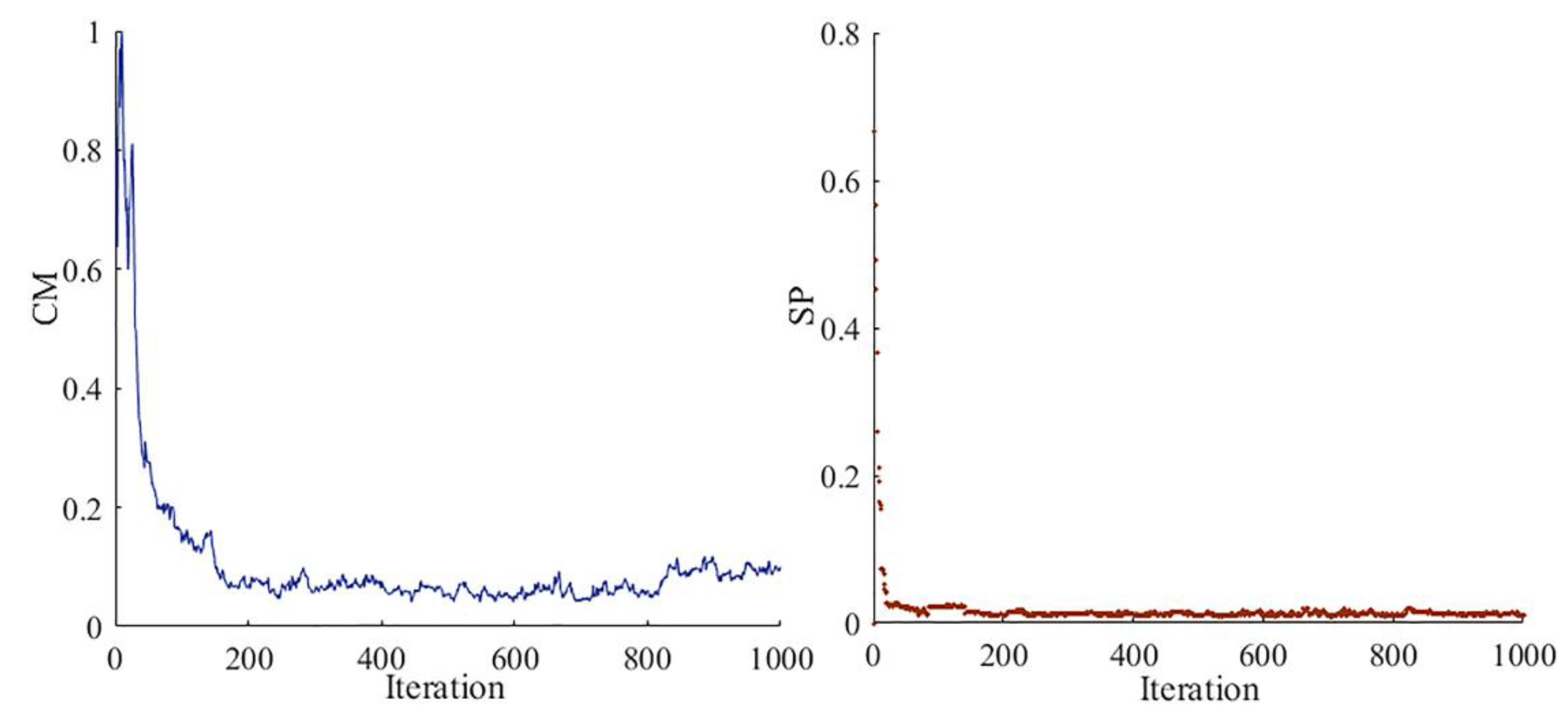
3.4. Performance Indicators

3.4.1. Convergence

We select the convergence metric ($CM$) and the uniformity metric ($SP$) to measure the performance of the NSPSO algorithm. Deb and Jain proposed an evaluation method based on the degree of approach [40], which calculates the minimum distance from the solution set to the reference set or the Pareto optimal set, to measure the algorithm’s convergence degree. The $CM$ values for each iteration are as follows:

$$C{M}_{gen}=C{P}_{gen}/C{P}_0$$

(29)

where

$$C{P}_{gen}=\frac{{\displaystyle \sum _{m\in M}\underset{p\in P^{*}}{\min }}\sqrt{{{\displaystyle \sum _{n\in N}\left(\frac{F_n{}_{,m}-F_{n,p}}{F_n^{\max }-F_n^{\min }}\right)}}^2}}{\left|M\right|}$$

(30)

A smaller $CM$ value means a faster convergence speed of the solution set, and vice versa.

3.4.2. Spacing

The spacing metric, proposed by Schott [41], can measure the distribution range of non-inferior solutions in the objective space by calculating the standard deviation of the distance between neighboring vectors of each solution.

$$SP=\sqrt{\frac{1}{M}{\displaystyle \sum _{m\in M}{(\overline{d}-d_m)}^2}}$$

(31)

A higher $SP$ value means that a more uniform distribution of the Pareto solutions is obtained. $SP=0$ represents the equidistant distribution of all solutions in the Pareto solution set.

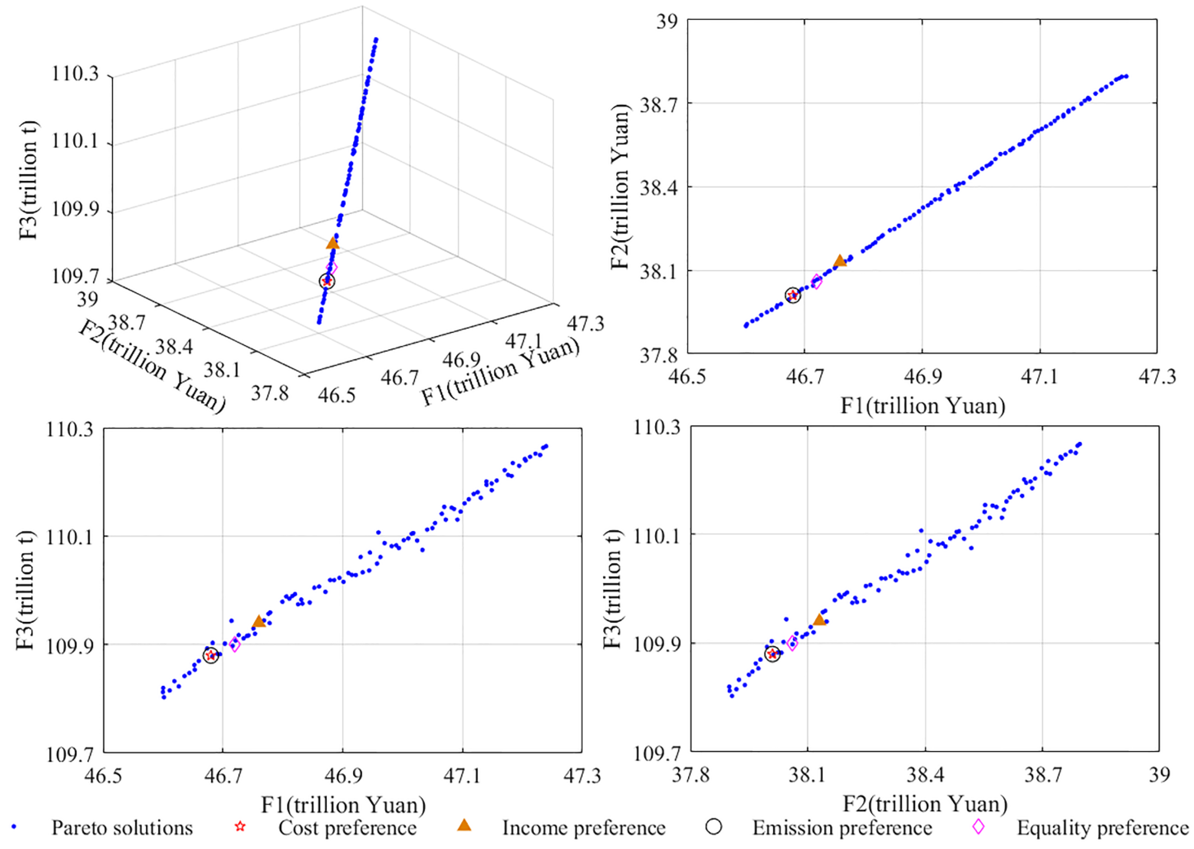
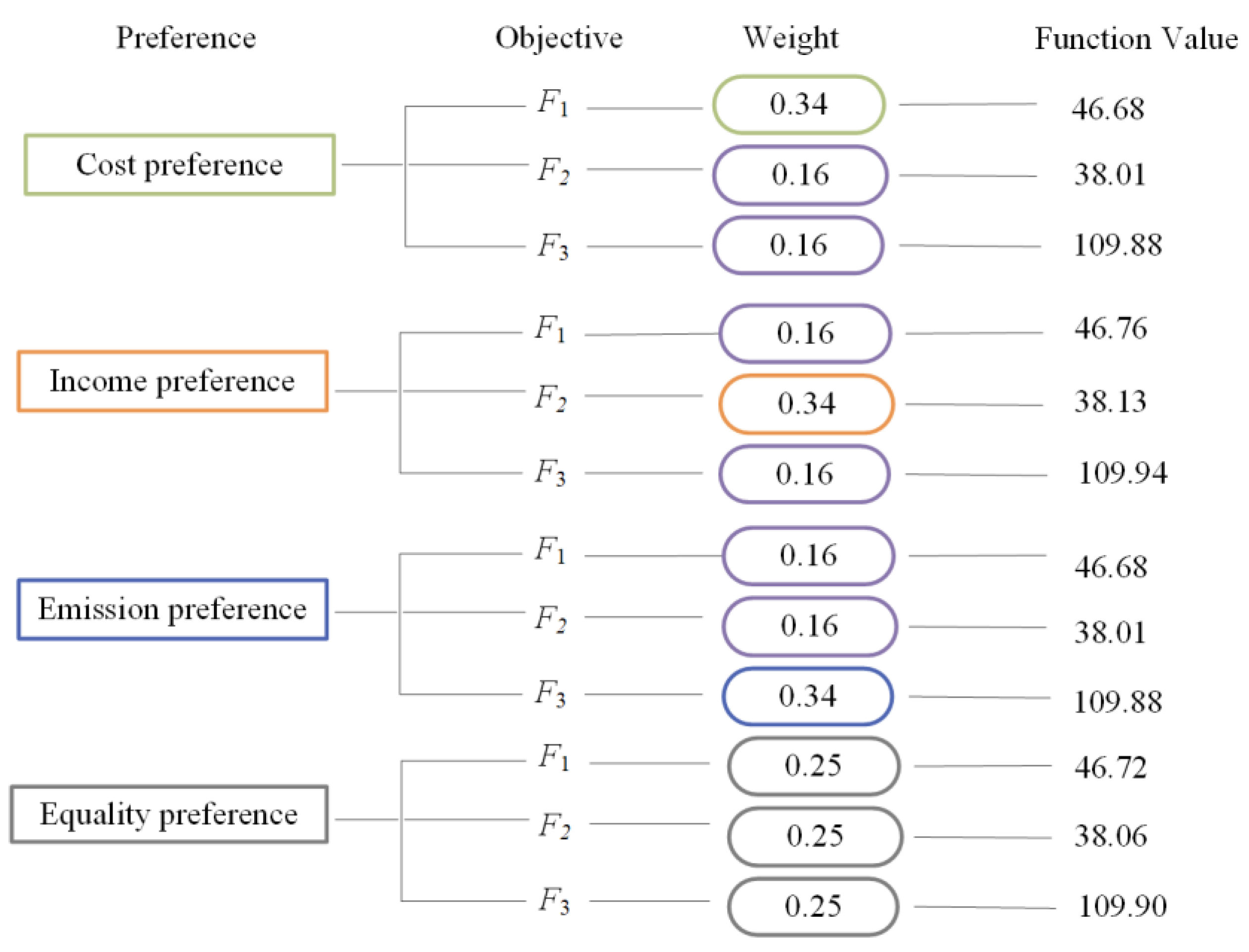
3.5. Selection of the Best Compromise Solution

The Pareto front obtained from the multi-objective problem is a set of non-dominated solutions satisfying constraints. Due to the trade-off between objectives, not all objectives will reach the unique optimal value. In practical problems, it is necessary to combine decision-makers’ preferences to select the non-inferior solution to obtain the final optimal solution. The present study applies the integrated method (SC–MTD–GAM) consisting of subtractive clustering (SC), multi-criteria tournament decision (MTD), and gain analysis method (GAM) to select the best trade-off solutions on the optimal Pareto fronts [42].

In the SC–MTD–GAM method, we first use SC to divide the normalized non-inferior solution set into different clusters according to the distance of each solution in the objective space. Then, the nearest solution to the ideal point is selected as the representative solution for each cluster. Second, MTD is used to calculate the score of each representative solution in each criterion (i.e., objective). The ranking matrix under each preference is calculated by the minimum index method combined with the weight obtained from the decision preference, with the first ranking considered the satisfactory solution. The decision-makers’ preference is reflected by prioritizing objectives, and the smaller the value, the more attention is paid to the objective. For example, preference matrix $\rho =[1,2,2]$ means that decision-makers consider $F_1$ to be more important than $F_2$, and $F_3$, $F_2$, and $F_3$ are equally important. Then, the given preference is transformed into a weight by multiplicative preference relation. Finally, by comparing the losses and gains of the candidate solutions in the first ranking under each preference, we obtain final solutions that can replace the solutions acquired by MTD under each preference.

Combined with model construction, solution, and final solution selection, we show the final framework of the proposed stochastic nonlinear multi-objective model in Figure 1.

4. China’s Power Generation Source Optimization

4.1. Data and Parameter Settings

4.1.1. Data

All the data are from yearbooks, reports, or publications. For example, each power generation source’s historical cumulative installed capacity and annual average usage hours are from the China Electric Power Yearbook. The GDP and electricity consumption data are from the China Statistical Yearbook. The on-grid price of the power generation source is derived from the National Electricity Price Regulation Bulletin. The learning rate of LCOE and life cycle carbon emissions are referred to in the studies of Yi et al. [27], Wang et al. [43], and Wu et al. [44]. More details of the data and their sources are listed in Appendix A,

Table A2. Installed potential of nuclear power in each province.

Installation	Provinces, Municipalities or Autonomous Regions
Already installed	Liaoning, Shandong, Jiangsu, Zhejiang, Fujian, Guangdong, Guangxi, Hainan
Planned installation	Jilin, Anhui, Jiangxi, Henan, Hubei, Hunan, Chongqing, Sichuan Gansu, Qinghai
No installation conditions	Shanghai, Beijing, Tianjin, Hebei, Shanxi, Heilongjiang, Inner Mongolia, Yunnan, Guizhou, Shaanxi, Ningxia, Tibet, Xinjiang

.

4.1.2. Model Parameters

The base year of this study is 2016, and the power generation structure for 2017 to 2040 is optimized. The historical data for the parameters involved were obtained from various yearbooks, reports, or published literature. According to their characteristics, parameters are set by different methods of fitting function, linear interpolation, and literature reference. The specific values and setting methods are shown in

Table 1. Values and setting methods of model parameters.

Parameters	Values	Setting Methods or References
$r$	$r=0.05$	The people’s Bank of China
${\eta }_{i,1,t}$	${\eta }_{i,1,t}=0.0098$	Average value of from 2011 to 2016
$h_{i,j,t}$	$h_{1,1,t}=4519$$,h_{2,1,t}=4917.6$$,\text{…},h_{31,7,t}=2845$	Average value of from 2012 to 2016, PV and biomass takes the value of base year
$l{r}_t$	$l{r}_1=0.18$$,l{r}_3=0.1$$,l{r}_4=0$$,l{r}_5=0.13$$,l{r}_6=0.18$$,l{r}_7=0.15$	Yi et al. [27]
$\theta$	$\theta =0.02$	Wang and Lei [28]
$\lambda$	$\lambda =0.74$	Zhang et al. [45]
$s_{i,t}$	$s_{1,t}=0.021$$,s_{2,t}=0.024$$,s_{3,t}=0.001$$,s_{4,t}=0.014$$,s_{5,t}=0.001$$,s_{6,t}=0.006$$,s_{7,t}=0.045$	NEEDS [46]
$o_t$	$o_1=38$$,o_4=51$$,o_9=86$	De et al. [47] and Slater et al. [48]
$u_{i,t}$	$u_{1,t}=0.09$$,u_{6,t}=0.12$$,u_{9,t}=0.1$$,\text{…},u_{31,t}=0.12$	Feihong [49]
$a_{i,j,t}$	$a_{1,1,1}=0.43$$,a_{1,1,2}=0.41$$,\text{…},a_{31,7,24}=0$	Estimated by data from 2013–2016
$e{l}_j$	$e{l}_1=899.9$$,e{l}_2=90$$,e{l}_3=11.8$$,e{l}_4=3.92$$,e{l}_5=30.6$$,e{l}_6=36.8$$,e{l}_7=64$	Wang et al. [43], Wu et al. [44], and He et al. [50]
$l_{i,t}$	$l_{1,t}=0.071$$,l_{2,t}=0.067$$,l_{3,t}=0.069$$,\text{…},l_{31,t}=0.09$	Average value of data from 2012 to 2016
$b_{i,t}$	$b_{1,1}=0.04$$,b_{2,1}=0.04$$,b_{3,1}=0.1$$,\text{…},b_{31,24}=0.2$	Estimated by data from 2005–2016
$gd{p}_{i,t_0}$	$gd{p}_{1,t_0}=6.8$$,gd{p}_{2,t_0}=9.1$$,gd{p}_{3,t_0}=6.8$$,\text{…},gd{p}_{31,t_0}=7.6$	CNBS [51]
${\gamma }_{i,t}$	${\gamma }_{1,1}=6.5$$,{\gamma }_{2,1}=8.5$$,{\gamma }_{3,1}=7$$,\text{…},{\gamma }_{31,24}=4.1$	Estimated by data from 2005–2016
$G_{i,j}$	$G_{1,3}=3.5$$,G_{2,3}=0.04$$,\text{…},G_{31,7}=10.9$	Li and Shi [52], Song et al. [53], and Wang and Shan [54]
$w_{i,t}$	$w_{1,1}=205.3$$,w_{1,2}=201.1$$,\text{…},w_{31,24}=133.6$	Estimated by data from 2012–2016
$\mu$	$\mu =0.32$	Wang and Du [28]
${\tau }_t$	${\tau }_t=3$	Guo et al. [55]
${\phi }_t$	${\phi }_4=0.39$$,{\phi }_9=0.43$$,{\phi }_{14}=0.47$$,\text{…},{\phi }_{24}=0.55$	4% increase every five years
$\delta$	$\delta =0.047$	Average value of from 2012 to 2016
$P{L}_{k,t}$	$P{L}_{1,1}=193.1$$,P{L}_{1,2}=201.2$$,P{L}_{1,3}=209.3$$,\text{…},P{L}_{6,24}=313.1$	Estimated by data from 2010–2016
$\varphi$	$\varphi =0.12$	Minimum of international standard 12–25%
$L{T}_i$	$L{T}_1=30$$,L{T}_2=40$$,L{T}_3=60$$,L{T}_4=70$$,L{T}_5=20$$,L{T}_6=20$$,L{T}_7=20$	Yi et al. [27]

. In particular, we assume that the utilization hours of wind and PV power generation follow a uniform distribution with the maximum and minimum values of their historical phases as parameters based on the historical data. Since the utilization hours of wind and PV power are affected by climate, and the climate in a particular location does not change dramatically, the utilization hours can be considered equally distributed between the above maximum and minimum.

4.1.3. Algorithm Parameters

The NSPSO parameters are listed in

Table 2. NSPSO algorithm parameters and values.

Parameter	Description	Value
$Pop$	The size of the population	100
$Maxiter$	The maximum number of iterations	1000
$c_1,c_2$	cognitive coefficient and social coefficient	0.8
$W_{\min },W_{\max }$	The minimum and maximum inertia coefficient	0.1, 1.2

. The maximum number of iterations is the stopping criteria. The minimum and maximum of the inertia coefficient are used to calculate the inertia weight and determine the influence of the particle’s previous velocity on the current velocity.

$Pop$$Maxiter$$c_1,c_2$$W_{\min },W_{\max }$ The premise of using Monte Carlo simulation is to determine the number of simulations. Theoretically speaking, when the number of Monte Carlo simulations tends to be infinite, the expected value of the stochastic simulation is equal to its real value. However, due to the limitations of computing resources, a large enough number is usually set to approximate the real value in practical applications. By running different MCS samples (50, 100, 150, 250, 500), the final selected number is 150. This is because increasing the number of simulations does not result in significant changes in the results but increases the calculation time.

4.2. Results and Discussion

4.2.1. Performance Analysis

NSPSO solves the proposed model to obtain the optimal Pareto front. Fifty independent runs of the Matlab program were carried out in the same parameter and computing setting. Two metrics, convergence measure ($\mathrm{CM}$) and spacing ($\mathrm{SP}$), measure the convergence and uniformity of solutions in the front, respectively. The mean values of $\mathrm{CM}$ and $\mathrm{SP}$ are 0.18 and 0.02, respectively, and are listed in

Table 3. Statistical performance information (50 independent runs).

Indicators	Average	Standard Deviation	Best	Worst
$\mathrm{CM}$	0.18	0.13	0.11	0.23
$\mathrm{SP}$	0.02	0.04	0.02	0.05

. The values that best approximate the average value of $\mathrm{CM}$ and $\mathrm{SP}$ are taken as an example to show evaluation changes through iterations and the performance of two metrics, as shown in Figure 2. We see that $\mathrm{CM}$ and $\mathrm{SP}$ tend to be stable with iterations, indicating that the solution set converges and there is uniform distribution.

4.2.2. Final Solution Selection

Taking the independent run that best approximates the average value as an example, we selected alternative solutions on the Pareto front. First, 38 clusters and their representative solutions were selected according to the SC method and combined with weights, as shown in Figure 3. As shown in Figure 4, four solutions under different preferences were selected by MTD-GAM. Units $F_1$, $F_2$, and $F_3$ are, respectively, billion yuan, billion yuan, and million tonnes.

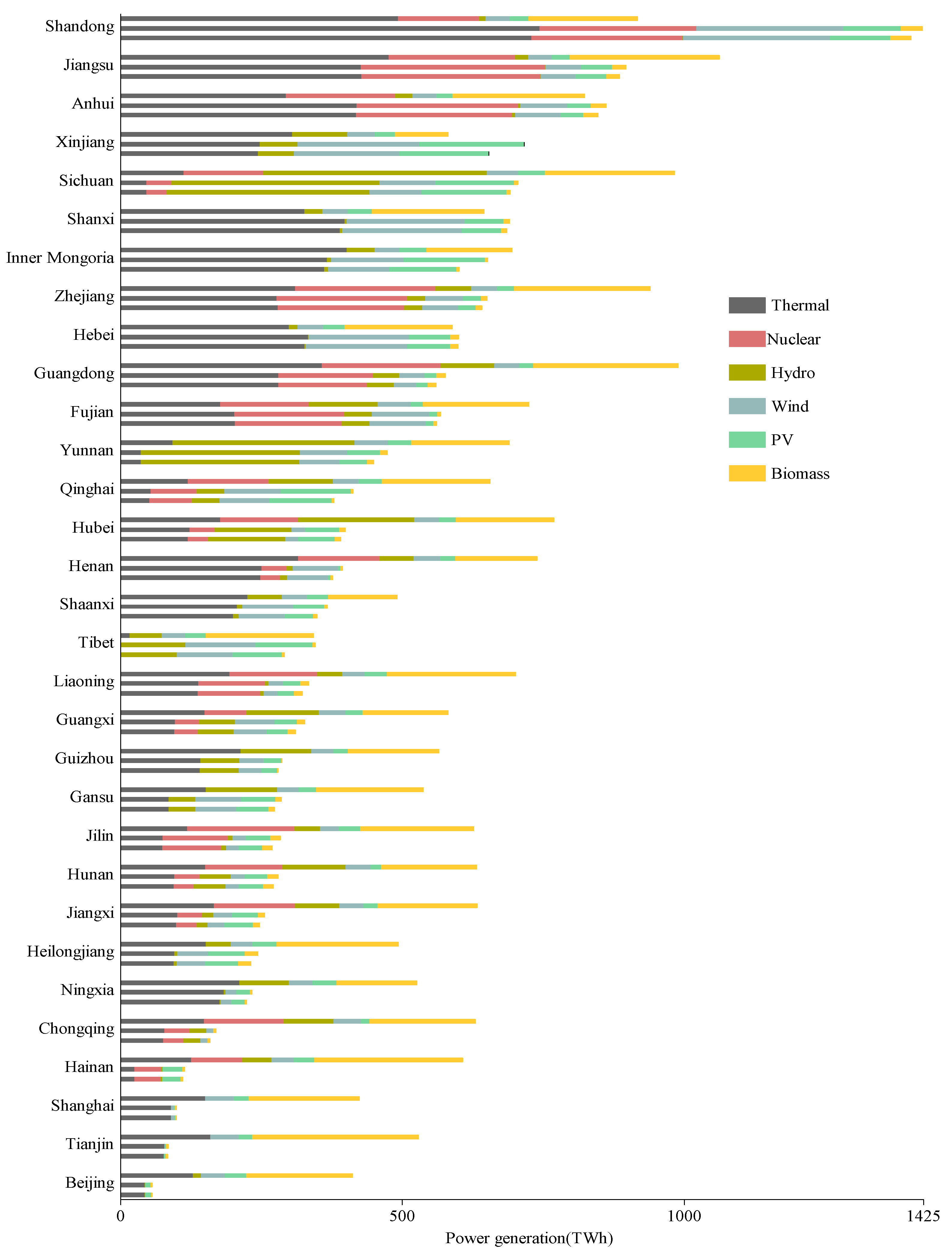
4.2.3. Optimized Power Generation Mix

We took the optimization results for equality preference as an example to further analyze. After optimization, the optimal power generation structure of China is thermal (41.7%), wind (17.1%), nuclear (15.6%), PV (12.4%), hydro (10.9%), and biomass (2.3%) in 2040. Renewable power generation in 14 provinces, including Heilongjiang and Qinghai, will account for 62.1% of total power generation, exceeding the thermal power generation share (Figure 5a). Solar PV power generation represents the highest proportion among all renewable power in these 14 provinces, at 30.21%. On the contrary, the average share of thermal power of total power generation in the other 17 provinces dropped from 83.6% in 2016 to 58.5% in 2040. However, thermal power still dominates the power generation structures (Figure 5b). These results are consistent with Zhang et al.’s finding that old and inefficient coal capacities are eliminated; low emission units are favored and more capacities will be constructed in China [56].

From 2016 to 2040, the annual average growth rate of non-hydro renewable power generation in 31 provinces is expected to be 12.06%; the growth rates for solar PV and wind power, in particular, are expected to be 17.95% and 10.62%, respectively (Figure 6). Tibet and Heilongjiang show the largest growth rates for wind power and solar PV generation, with average annual growth rates of 48.15% and 35.53%, respectively. Thermal power generation still has a 1.08% average annual growth rate because of the continuous growth in power demand but shows the largest average annual decline of 0.24% in Guangdong. Jiangsu followed, with an average annual decline of 0.13%. The research conducted by Gong et al. [57] also showed that the proportion of coal power in Jiangsu dropped significantly, from 72.7% to 48.7% in 2021–2050 under the BAU scenario.

Regarding cumulative installed capacity in service of the optimized power generation structure, the total installed capacity of thermal power is expected to rise gradually from 1062 GW in 2016 to 1326.33 GW in 2040, with an increase of 24.89%. Thermal power units equipped with carbon capture equipment are expected to increase from zero in 2016 to 421.11 GW in 2040, accounting for 31.75% of the cumulative installed capacity in service, as shown in Figure 7. Existing units with CC retrofitting reached 80.29 GW, composing 7.56% of the total installed capacity in service in 2016. Newly installed units equipped with CC equipment will reach 340.82 GW by 2040, with a share of 25.7% of the total installed capacity. These changes are similar to Zhang et al.’s [58] finding that coal power generation with carbon capture storage will play a considerable role in achieving China’s carbon neutrality target in the long term. CC needs to be deployed in large quantities after 2030 to substitute for traditional coal power.

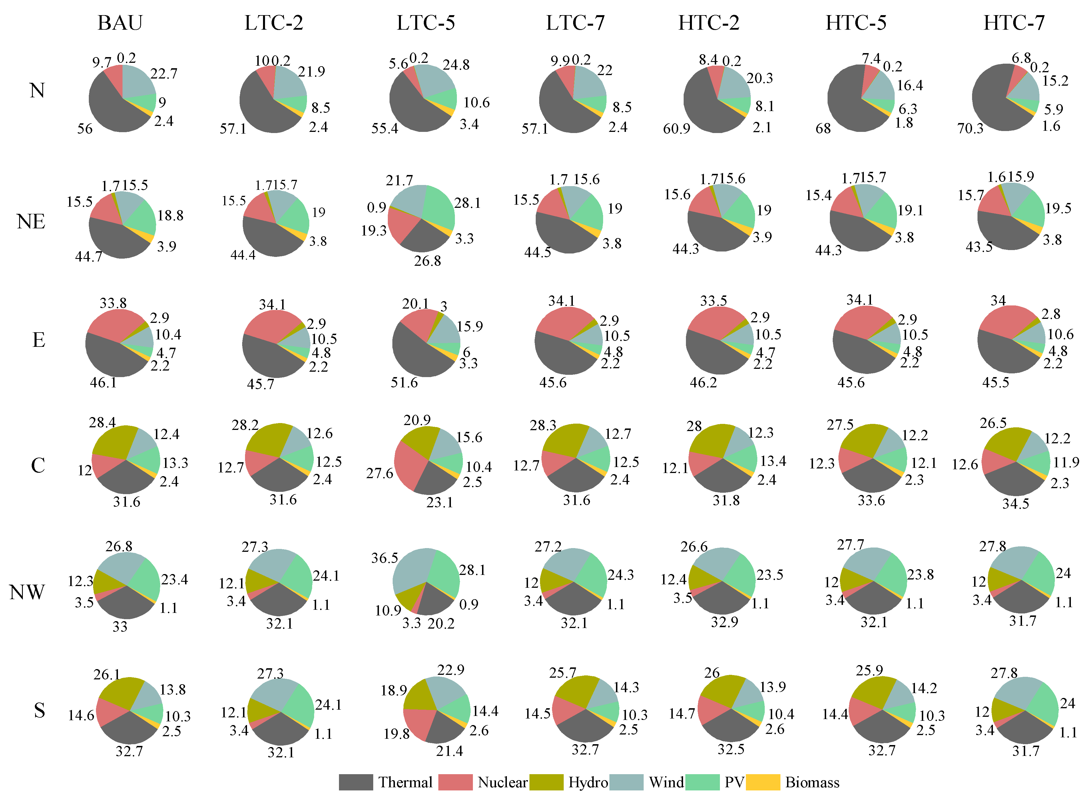
4.2.4. Effects of Regional Power Transmission Capacity on the Power Generation Source Mix

Interregional power transmission capacity is an important factor that affects the optimal regional power generation structure. However, future interregional power transmission capacity in China is uncertain. According to China’s current planning, only a few interregional transmission lines, such as the Qinghai-Henan line, the Sichuan-Jiangsu line, and the Sichuan-Zhejiang line, were planned in 2020. Referring to the interregional transmission capacity in Guo et al.’s study [55], which considers future government planning, we obtained the results in Section 4.2.2 as a business-as-usual scenario (BAU scenario). To further explore the influence of interregional power transmission capacity on the optimal power generation structure in China, we set up a low transmission capacity scenario (LTC scenario) and a high transmission capacity scenario (HTC scenario) by decreasing and increasing the transmission capacity in 2040 in the BAU scenario by 20%, 50%, and 70%. We named them LTC-2, LTC-5, LTC-7, HTC-2, HTC-5, and HTC-7. According to the collected historical data, the layout of inter-regional transmission lines in 2016 is shown in Figure 8. The transmission capacities of the six regions under each scenario are listed in Appendix A,

Table A3. Regional transmission capacity of seven scenarios in 2040.

Scenario	Direction	N	NE	E	C	NW	S
BAU	In (GW)	107.48	0.00	340.10	250.18	0.00	104.48
	Out (GW)	531.72	25.37	0.00	68.15	458.32	0.00
LTC-2 1	In (GW)	85.98	0.00	272.08	200.14	0.00	83.58
	Out (GW)	425.38	20.30	0.00	54.52	366.66	0.00
LTC-5	In (GW)	53.74	0.00	170.05	125.09	0.00	52.24
	Out (GW)	265.86	12.69	0.00	34.08	229.16	0.00
LTC-7	In (GW)	53.74	0.00	170.05	125.09	0.00	52.24
	Out (GW)	265.86	12.69	0.00	34.08	229.16	0.00
HTC-2 1	In (GW)	128.98	0.00	408.12	300.22	0.00	125.38
	Out (GW)	638.06	30.44	0.00	81.78	549.98	0.00
HTC-5	In (GW)	161.22	0.00	510.15	375.27	0.00	156.72
	Out (GW)	797.58	38.06	0.00	102.23	687.48	0.00
HTC-7	In (GW)	182.72	0.00	578.17	425.31	0.00	177.62
	Out (GW)	903.92	43.13	0.00	115.86	779.14	0.00

¹ HTC and LTC represent high and low transmission capacity scenarios, respectively.

.

Compared with the BAU scenario, the total power generation of provinces in the northwest grid areas increased significantly, from 2358.98 TWh to 5541.03 TWh in the LTC-5 scenario, with an increase of 134.89%, as shown in Figure 9. Among the provinces, the share of wind power generation increases by 36.33%, which is the biggest increase, and the share of thermal power generation decreases by 38.61%. In addition, the share of nuclear power generation and hydropower generation decrease by 5.71% and 11.38%, respectively, because, in the face of the limited power transmission capacity, the better choice for Northwest China is to develop its advantageous wind power photovoltaic power generation resources. Similarly, the largest decline in the share of thermal power generation occurs in the northeastern grid areas in the LTC-5 scenario, where the share decreases by 39.98%, from 44.7% to 26.83%. With the excellent foundation and potential of nuclear power development in Northeast China, the share of nuclear power generation increased by 24.52% when the regional transmission capacity decreased. Shares of nuclear power generation in Central China show varying growth under different scenarios. Among all scenarios, that share increases most in the LTC-5 scenario, reaching 130%, which is consistent with the planning of taking inland nuclear power plants as an important power resource in Central China in the future. Among all power sources, the proportion of photovoltaic power generation in the provinces of the southern power grid has the largest change in the LTC-2 scenario, from 10.34% to 24.05%, an increase of 132.59%.

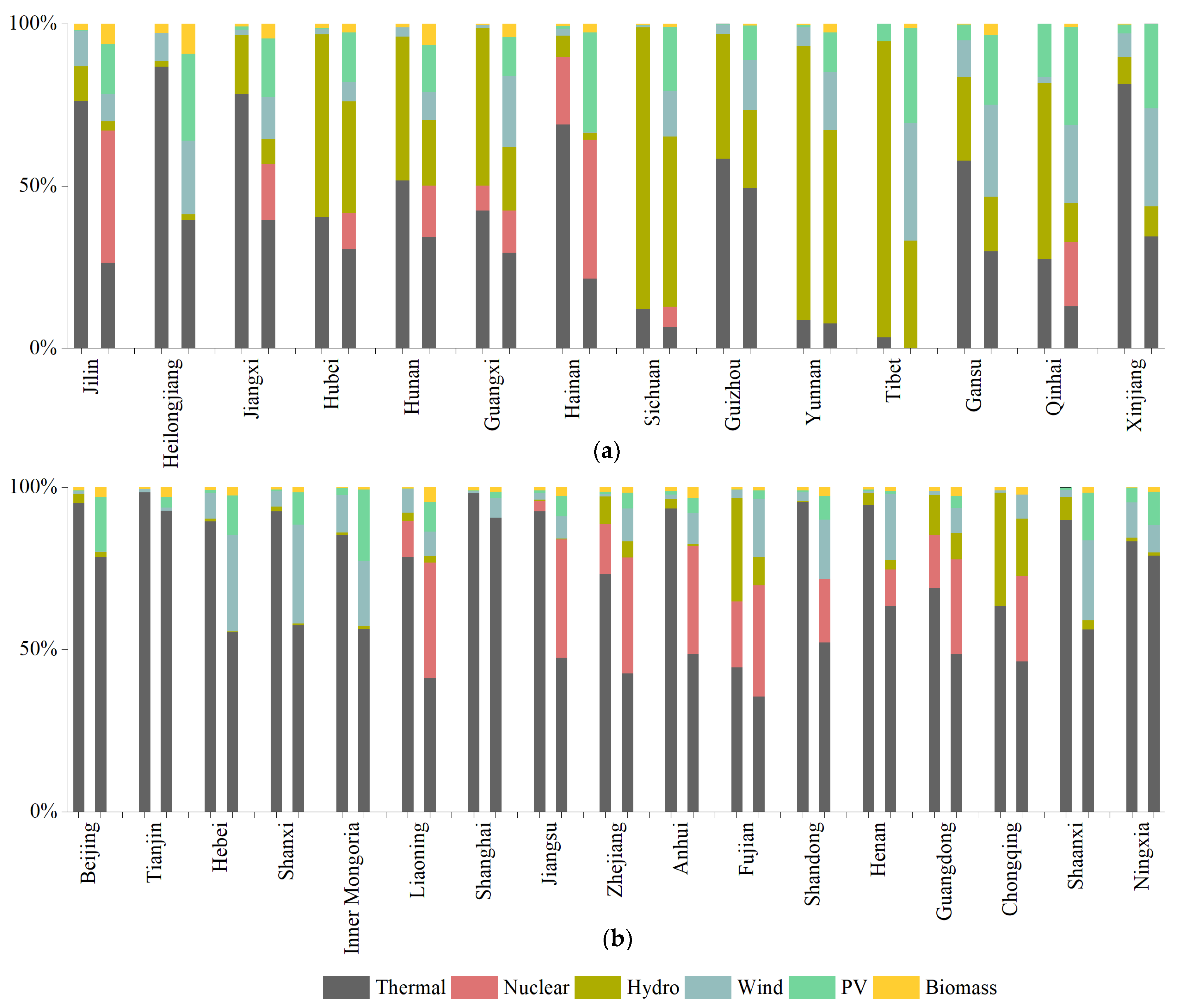
4.2.5. Effects of Regional Power Consumption Demand on the Power Generation Source Mix

The premise of power generation-mix optimization is to directly meet the power demand that directly affects the final installed capacity of the power generation source. The growth rate of provincial GDP is an important factor affecting power demand [59]. Therefore, we set up two scenarios, low GDP growth rate (the LGDP scenario) and high GDP growth rate (the HGDP scenario), based on the BAU scenario set in Section 4.2 and shown in Appendix A,

Table A4. Different scenarios of provinces’ GDP growth.

Province	2016–2020				2021–2025			2026–2030			2031–2035			2036–2040
	HGDP	BAU	LGDP	HGDP	BAU	LGDP	HGDP	BAU	LGDP	HGDP	BAU	LGDP	HGDP	BAU	LGDP
Beijing	6.5	5.8	4.8	6.0	5.0	4.0	5.2	4.2	3.2	4.4	3.4	2.4	3.6	2.6	1.6
Tianjin	8.5	7.8	6.8	8.0	7.0	6.0	7.2	6.2	5.2	6.4	5.4	4.4	5.6	4.6	3.6
Hebei	7.0	6.3	5.3	6.5	5.5	4.5	5.7	4.7	3.7	4.9	3.9	2.9	4.1	3.1	2.1
Shanxi	6.5	5.8	4.8	6.0	5.0	4.0	5.2	4.2	3.2	4.4	3.4	2.4	3.6	2.6	1.6
Inner Mongolia	7.5	6.8	5.8	7.0	6.0	5.0	6.2	5.2	4.2	5.4	4.4	3.4	4.6	3.6	2.6
Liaoning	6.6	5.9	4.9	6.1	5.1	4.1	5.3	4.3	3.3	4.5	3.5	2.5	3.7	2.7	1.7
Jilin	6.5	5.8	4.8	6.0	5.0	4.0	5.2	4.2	3.2	4.4	3.4	2.4	3.6	2.6	1.7
Heilongjiang	6.0	5.3	4.3	5.5	4.5	3.5	4.7	3.7	2.7	3.9	2.9	1.9	3.1	2.1	1.1
Shanghai	6.5	5.8	4.8	6.0	5.0	4.0	5.2	4.2	3.2	4.4	3.4	2.4	3.6	2.6	1.6
Jiangsu	7.5	6.8	5.8	7.0	6.0	5.0	6.2	5.2	4.2	5.4	4.4	3.4	4.6	3.6	2.6
Zhejiang	7.0	6.3	5.3	6.5	5.5	4.5	5.7	4.7	3.7	4.9	3.9	2.9	4.1	3.1	2.1
Anhui	8.5	7.8	6.8	8.0	7.0	6.0	7.2	6.2	5.2	6.4	5.4	4.4	5.6	4.6	3.6
Fujian	8.5	7.8	6.8	8.0	7.0	6.0	7.2	6.2	5.2	6.4	5.4	4.4	5.6	4.6	3.6
Jiangxi	8.5	7.8	6.8	8.0	7.0	6.0	7.2	6.2	5.2	6.4	5.4	4.4	5.6	4.6	3.6
Shandong	7.5	6.8	5.8	8.0	6.0	5.0	6.2	5.2	4.2	5.4	4.4	3.4	4.6	3.6	2.6
Henan	8.0	7.3	6.3	7.5	6.5	5.5	6.7	5.7	4.7	5.9	4.9	3.9	5.1	4.1	3.1
Hubei	8.5	7.8	6.8	8.0	7.0	6.0	7.2	6.2	5.2	6.4	5.4	4.4	5.6	4.6	3.6
Hunan	8.5	7.8	6.8	8.0	7.0	6.0	7.2	6.2	5.2	6.4	5.4	4.4	5.6	4.6	3.6
Guangdong	7.0	6.3	5.3	6.5	5.5	4.5	5.7	4.7	3.7	4.9	3.9	2.9	4.1	4.1	3.1
Guangxi	7.5	6.8	5.8	7.0	6.0	5.0	6.2	5.2	4.2	5.4	4.4	3.4	4.6	4.6	3.6
Hainan	7.0	6.3	5.3	6.5	5.5	4.5	5.7	4.7	3.7	4.9	3.9	2.9	4.1	3.1	2.1
Chongqing	9.0	8.3	7.3	8.5	7.5	6.5	7.7	6.7	5.7	6.9	5.9	4.9	6.1	5.1	4.1
Sichuan	7.0	6.3	5.3	6.5	5.5	4.5	5.7	4.7	3.7	4.9	3.9	2.9	4.1	3.1	2.1
Guizhou	10.0	9.3	8.3	9.5	8.5	7.5	8.7	7.7	6.7	7.9	6.9	5.9	7.1	6.1	5.1
Yunnan	8.5	7.8	6.8	8.0	7.0	6.0	7.2	6.2	5.2	6.4	5.4	4.4	5.6	4.6	3.6
Tibet	10.0	9.3	8.3	9.5	8.5	7.5	8.7	7.7	6.7	7.9	6.9	5.9	7.1	6.1	5.1
Shannxi	8.0	7.3	6.3	7.5	6.5	5.5	6.7	5.7	4.7	5.9	4.9	3.9	5.1	4.1	3.1
Gansu	7.5	6.8	5.8	7.0	6.0	5.0	6.2	5.2	4.2	5.4	4.4	3.4	4.6	3.6	2.6
Qinghai	7.5	6.8	5.8	7.0	6.0	5.0	6.2	5.2	4.2	5.4	4.4	3.4	4.6	3.6	2.6
Ningxia	7.5	6.8	5.8	7.0	6.0	5.0	6.2	5.2	4.2	5.4	4.4	3.4	4.6	3.6	2.6
Xinjiang	9.0	8.3	7.3	8.5	7.5	6.5	7.7	6.7	5.7	6.9	5.9	4.9	6.1	5.1	4.1

.

Figure 10 shows that Shandong, Anhui, Shanxi, Hebei, Xinjiang, and Tibet have maximum power generation under the BAU scenario, while the other 25 provinces have maximum power generation in the HGDP scenario. Compared with the BAU scenario, the largest change in total power generation is in Beijing under the HGDP scenario, increasing by 639.7%. Among all power generation sources, Beijing’s wind power accounts for the most significant increase in its total power generation, from 0.2% to 10.5%, an increase of 4665.6%. The proportion of thermal power in the total power generation will drop by 60.2% in 2040.

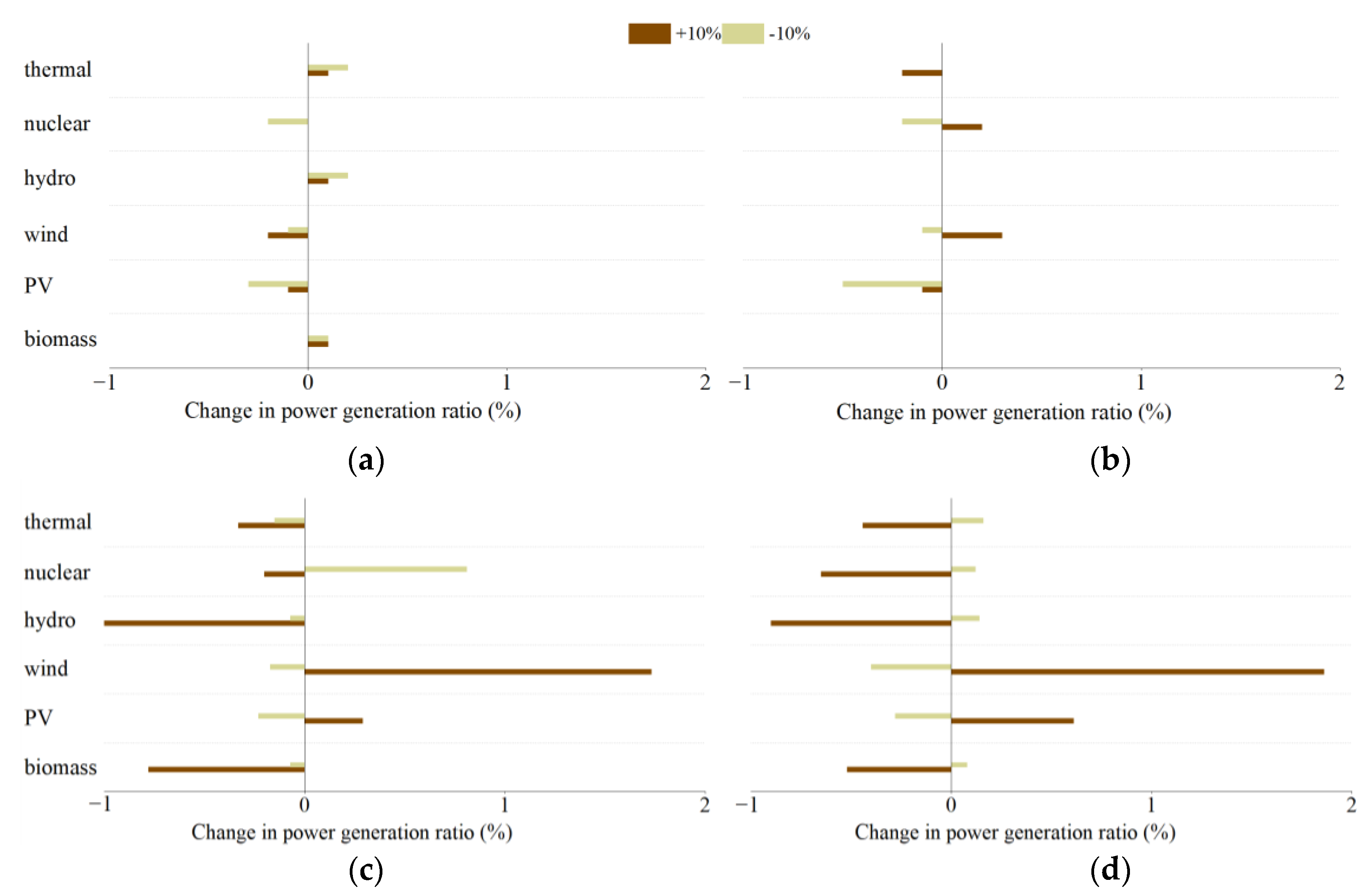
4.3. Sensitivity Analysis

To explore the influence of some key parameters of the proposed model on the solution, we selected four important parameters (non-carbon external cos, LCOE learning rate, supply reserve factor, and the share of non-fossil energy in total installed capacity) that have significant uncertainty and may affect the optimization results. The values of the four parameters were added and reduced by 10% to explore the effects on the optimal power generation structure.

In general, the optimal power generation structure is not sensitive to changes in the four parameters, as shown in Figure 11. The growth rate in the share of generation changes less than 2% when the parameter value increases or decreases by 10%. Specifically, the maximum changing rate is apparent when the share of non-fossil energy in the total installed capacity increases by 10% and the share of wind power generation decreases by 1.86%.

5. Conclusions

We proposed a new stochastic nonlinear multi-objective model to establish a suitable framework for a future power system with high renewable energy penetration. We applied the model to obtain the optimal power installation roadmap and power generation mix of six power sources in 31 provinces in China from 2017 to 2040. We conclude the following from the results:

(a)

The proposed model meets the stochastic nonlinear multi-objective decision-making requirements of power source mix optimization under variable renewable integration. In the model, MCS effectively simulates the uncertainty of variable renewable energy output. Nonlinear formulation successfully describes the complex relationship between each power source’s LCOE and installed capacity.

(b)

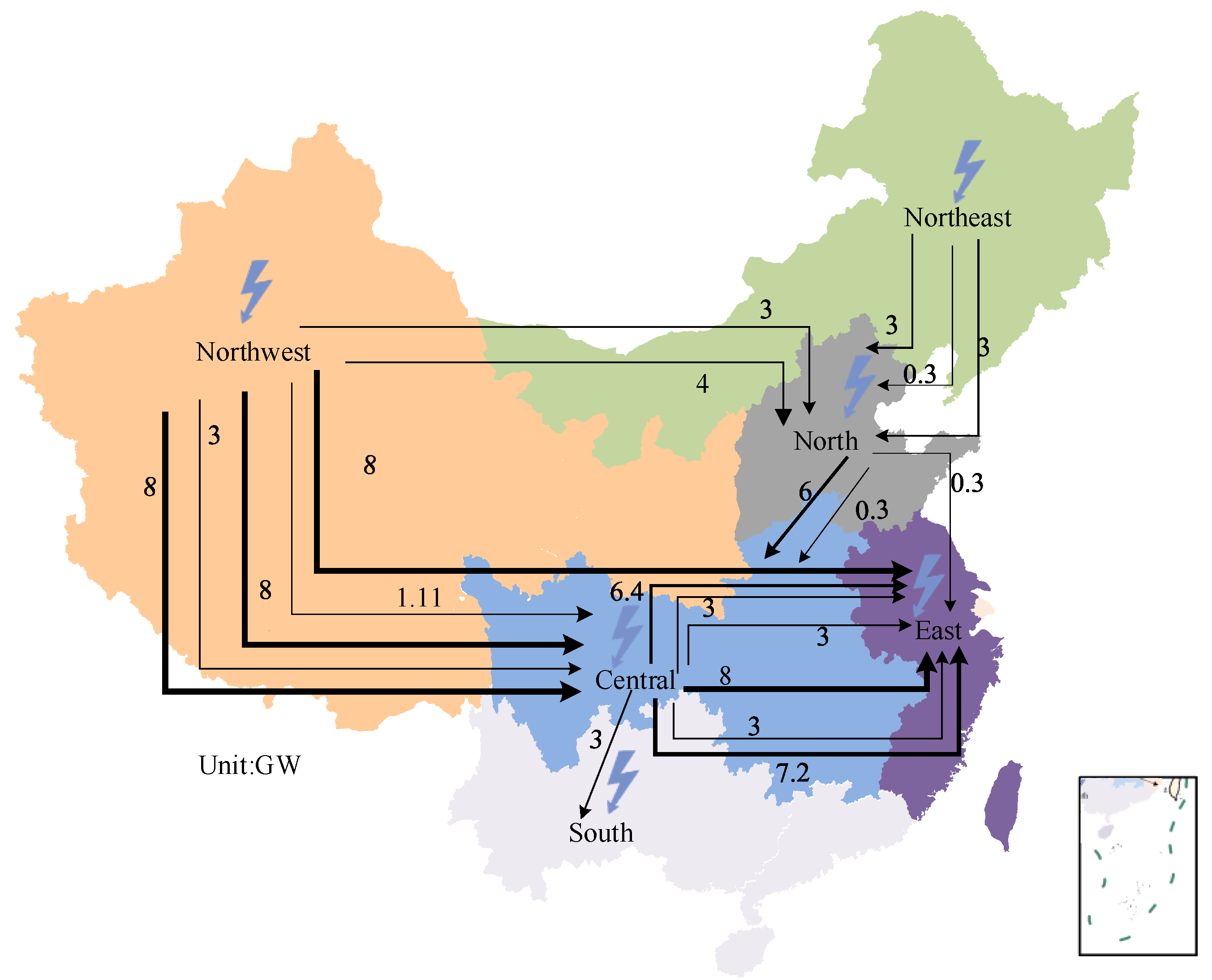
The proposed model integrated power transmission capacity constraints and set different scenarios for transmission capacity, which can better capture a region’s characteristics and avoid inadequate or excessive power installation more effectively than the traditional power structure optimization model. It provides a more feasible installation decision plan and obtains a more realistic optimal power generation structure. The results show that a 50% reduction in interregional power transmission capacity increases 134.9% in the total power generation in the southern grid area. At the same time, the reduction in interregional power transmission capacity caused a decline in the proportion of thermal power generation in the areas that mainly transmit power to others.

(c)

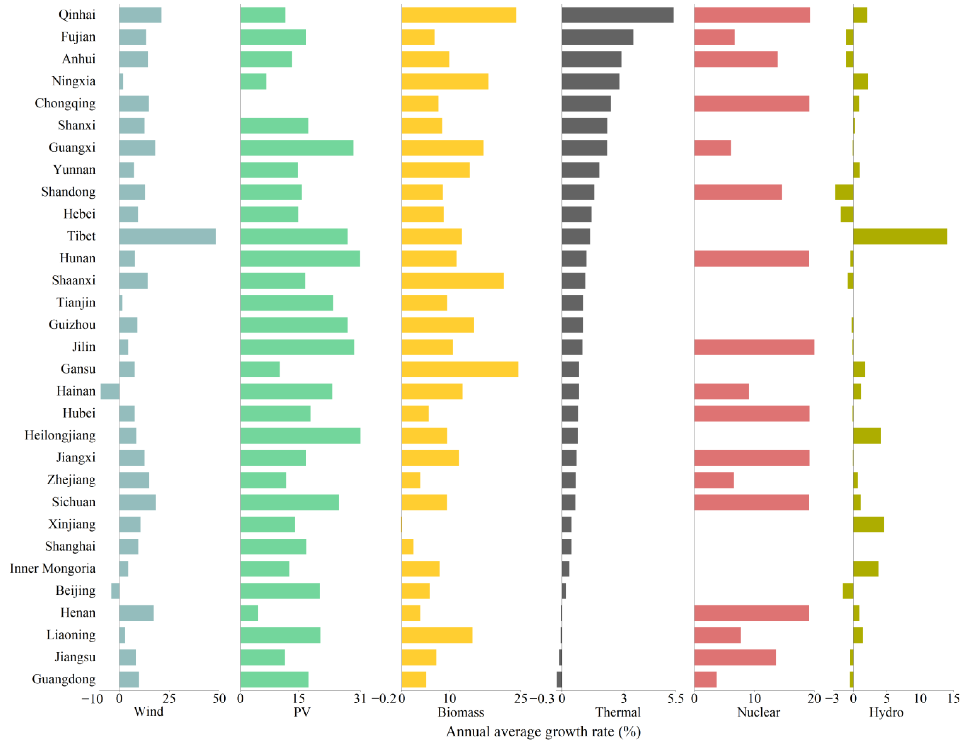
By 2040, the share of clean power in China’s optimal power generation structure will exceed 58%, achieved by transforming power generation to low carbonization. According to the results, clean electricity in China will reach 58.3% of total power production, including wind (17.1%), nuclear (15.6%), PV (12.4%), hydro (10.9%), and biomass (2.3%), which is an increase of 135.1% over 2016. While the proportion of thermal power decreased from 71.8% to 41.7% among all the provinces, 14 of them, including Heilongjiang, Sichuan, and Qinghai, accounted for more renewable electricity generation than thermal power. In particular, the average share of PV power generation in these provinces was as high as 30.2%. However, the other 17 provinces, including Beijing, Tianjin, and Hebei, were still dominated by thermal power.

(d)

According to the sensitivity analysis, the optimization results are not sensitive to the four key model parameters, such as the non-carbon external cost, the LCOE learning rate, the reserve factor, and the share of non-fossil energy in the total installed capacity. The growth rate in the share of power generation changes less than 2% when the parameter value increases or decreases by 10%.

References

1. IEA. Global Energy & CO2 Status Report; IEA: Paris, France, 2019. [Google Scholar]
2. Thangavelu, S.R.; Khambadkone, A.M.; Karimi, I.A. Long-term optimal energy mix planning towards high energy security and low GHG emission. Appl. Energy 2015, 154, 959–969. [Google Scholar] [CrossRef]
3. Kaushik, E.; Prakash, V.; Mahela, O.P.; Khan, B.; El-Shahat, A.; Abdelaziz, A.Y. Comprehensive overview of power system flexibility during the scenario of high penetration of renewable energy in utility grid. Energies 2022, 15, 516. [Google Scholar] [CrossRef]
4. Asiaban, S.; Kayedpour, N.; Samani, A.E.; Bozalakov, D.; De Kooning, J.D.M.; Crevecoeur, G.; Vandevelde, L. Wind and solar intermittency and the associated integration challenges: A comprehensive review including the status in the Belgian power system. Energies 2021, 14, 2630. [Google Scholar] [CrossRef]
5. Kahouli-Brahmi, S. Technological learning in energy–environment–economy modelling: A survey. Energy Policy 2008, 36, 138–162. [Google Scholar] [CrossRef]
6. Huang, H.; Hui, J.; Cai, W.; Wang, C. Optimizing the power generation structure for low carbon development target in China: A comparison study of endogenous and exogenous technology improvements. Energy Procedia 2019, 158, 4055–4060. [Google Scholar] [CrossRef]
7. Yao, Y.; Xu, J.-H.; Sun, D.-Q. Untangling global levelised cost of electricity based on multi-factor learning curve for renewable energy: Wind, solar, geothermal, hydropower and bioenergy. J. Clean. Prod. 2021, 285, 124827. [Google Scholar] [CrossRef]
8. Hobbs, B.F. Optimization methods for electric utility resource planning. Eur. J. Oper. Res. 1995, 83, 1–20. [Google Scholar] [CrossRef]
9. Park, Y.M.; Park, J.B.; Won, J.R. A hybrid genetic algorithm/dynamic programming approach to optimal long-term generation expansion planning. Int. J. Electr. Power Energy Syst. 1998, 20, 295–303. [Google Scholar] [CrossRef]
10. Wang, J.; Sparrow, F.T. The cost of uncertainty in capacity expansion problems. Int. J. Energy Res. 1999, 23, 1187–1198. [Google Scholar] [CrossRef]
11. Sadeghi, A.; Larimian, T. Sustainable electricity generation mix for Iran: A fuzzy analytic network process approach. Sustain. Energy Technol. Assess. 2018, 28, 30–42. [Google Scholar] [CrossRef]
12. Atabaki, M.S.; Aryanpur, V. Multi-objective optimization for sustainable development of the power sector: An economic, environmental, and social analysis of Iran. Energy 2018, 161, 493–507. [Google Scholar] [CrossRef]
13. Al Shidhani, T.; Ioannou, A.; Falcone, G. Multi-objective optimisation for power system planning integrating sustainability indicators. Energies 2020, 13, 2199. [Google Scholar] [CrossRef]
14. Junne, T.; Cao, K.-K.; Miskiw, K.K.; Hottenroth, H.; Naegler, T. Considering life cycle greenhouse gas emissions in power system expansion planning for Europe and North Africa using multi-objective optimization. Energies 2021, 14, 1301. [Google Scholar] [CrossRef]
15. Makhloufi, S.; Khennas, S.; Bouchaib, S.; Arab, A.H. Multi-objective cuckoo search algorithm for optimized pathways for 75% renewable electricity mix by 2050 in Algeria. Renew. Energy 2022, 185, 1410–1424. [Google Scholar] [CrossRef]
16. Luz, T.; Moura, P.; de Almeida, A. Multi-objective power generation expansion planning with high penetration of renewables. Renew. Sustain. Energy Rev. 2018, 81, 2637–2643. [Google Scholar] [CrossRef]
17. Yu, S.; Zhou, S.; Zheng, S.; Li, Z.; Liu, L. Developing an optimal renewable electricity generation mix for China using a fuzzy multi-objective approach. Renew. Energy 2019, 139, 1086–1098. [Google Scholar] [CrossRef]
18. Yu, S.; Zhou, S.; Qin, J. Layout optimization of China’s power transmission lines for renewable power integration considering flexible resources and grid stability. Int. J. Electr. Power Energy Syst. 2022, 135, 107507. [Google Scholar] [CrossRef]
19. Tekiner, H.; Coit, D.W.; Felder, F.A. Multi-period multi-objective electricity generation expansion planning problem with Monte-Carlo simulation. Electr. Power Syst. Res. 2010, 80, 1394–1405. [Google Scholar] [CrossRef] [Green Version]
20. Hytowitz, R.B.; Hedman, K.W. Managing solar uncertainty in microgrid systems with stochastic unit commitment. Electr. Power Syst. Res. 2015, 119, 111–118. [Google Scholar] [CrossRef]
21. Wang, C.; Ye, M.; Cai, W.; Chen, J. The value of a clear, long-term climate policy agenda: A case study of China’s power sector using a multi-region optimization model. Appl. Energy 2014, 125, 276–288. [Google Scholar] [CrossRef]
22. Hui, J.; Cai, W.; Wang, C.; Ye, M. Analyzing the penetration barriers of clean generation technologies in China’s power sector using a multi-region optimization model. Appl. Energy 2017, 185, 1809–1820. [Google Scholar] [CrossRef]
23. Chen, S.; Liu, P.; Li, Z. Multi-regional power generation expansion planning with air pollutants emission constraints. Renew. Sustain. Energy Rev. 2019, 112, 382–394. [Google Scholar] [CrossRef]
24. Daş, G.S.; Gzara, F.; Stützle, T. A review on airport gate assignment problems: Single versus multi objective approaches. Omega 2020, 92, 102146. [Google Scholar] [CrossRef]
25. Deb, K. Multi-objective optimization. In Search Methodologies; Springer: Berlin/Heidelberg, Germany, 2014; pp. 403–449. [Google Scholar]
26. Handayani, K.; Krozer, Y.; Filatova, T. From fossil fuels to renewables: An analysis of long-term scenarios considering technological learning. Energy Policy 2019, 127, 134–146. [Google Scholar] [CrossRef]
27. Yi, B.W.; Xu, J.H.; Fan, Y. Inter-regional power grid planning up to 2030 in China considering renewable energy development and regional pollutant control: A multi-region bottom-up optimization model. Appl. Energy 2016, 184, 641–658. [Google Scholar] [CrossRef]
28. Wang, X.; Du, L. Study on carbon capture and storage (CCS) investment decision-making based on real options for China’s coal-fired power plants. J. Clean. Prod. 2016, 112, 4123–4131. [Google Scholar] [CrossRef]
29. IEA. CO2 Emissions from Fuel Combustion 2018; IEA: Paris, France, 2018; p. 515. [Google Scholar]
30. Reimers, A.; Cole, W.; Frew, B. The impact of planning reserve margins in long-term planning models of the electricity sector. Energy Policy 2019, 125, 1–8. [Google Scholar] [CrossRef]
31. Pratama, Y.W.; Purwanto, W.W.; Tezuka, T.; McLellan, B.C.; Hartono, D.; Hidayatno, A.; Daud, Y. Multi-objective optimization of a multiregional electricity system in an archipelagic state: The role of renewable energy in energy system sustainability. Renew. Sustain. Energy Rev. 2017, 77, 423–439. [Google Scholar] [CrossRef]
32. Wang, F.; Yin, H.; Li, S. China’s renewable energy policy: Commitments and challenges. Energy Policy 2010, 38, 1872–1878. [Google Scholar] [CrossRef]
33. Mcintyre, T.J.; Kirby, B.J.; Kisner, R.A.; Van Dyke, J.W. Real Power Regulation for the Utility Power Grid via Responsive Loads. U.S. Patent 7,536,240, 19 May 2009. [Google Scholar]
34. NDRC. The 13th Five-Year Plan for Energy Development; NDRC: Beijing, China, 2016. [Google Scholar]
35. NDRC. The 13th Five-Year Plan for Electricity Development; NDRC: Beijing, China, 2016. [Google Scholar]
36. Vithayasrichareon, P.; MacGill, I.F. A Monte Carlo based decision-support tool for assessing generation portfolios in future carbon constrained electricity industries. Energy Policy 2012, 41, 374–392. [Google Scholar] [CrossRef]
37. Lei, D.; Yan, X. Multi-Objective Intelligent Optimization Algorithm and Application; Science Press: Beijing, China, 2009; p. 389. [Google Scholar]
38. Li, X. A Non-Dominated Sorting Particle Swarm Optimizer for Multi-Objective Optimization; Springer: Berlin/Heidelberg, Germany, 2003; pp. 37–48. [Google Scholar]
39. Deb, K. Multi-objective optimisation using evolutionary algorithms: An introduction. In Multi-Objective Evolutionary Optimisation for Product Design and Manufacturing; Springer: London, UK, 2011; pp. 3–34. [Google Scholar] [CrossRef]
40. Deb, K.; Jain, S. Running performance metrics for evolutionary multi-objective optimization. In Proceedings of the Fourth Asia-Pacific Conference on Simulated Evolution and Learning (SEAL’02), Singapore, 3 February 2002; pp. 13–20. [Google Scholar]
41. Schott, J.R. Fault Tolerant Design Using Single and Multicriteria Genetic Algorithm Optimization. Ph.D. Thesis, Massachusetts Institute of Technology, Cambridge, MA, USA, 1995. [Google Scholar]
42. Yu, S.; Zheng, S.; Gao, S.; Yang, J. A multi-objective decision model for investment in energy savings and emission reductions in coal mining. Eur. J. Oper. Res. 2017, 260, 335–347. [Google Scholar] [CrossRef]
43. Wang, L.; Wang, Y.; Zhou, Z.; Garvlehn, M.P.; Bi, F. Comparative assessment of the environmental impacts of hydro-electric, nuclear and wind power plants in China: Life cycle considerations. Energy Procedia 2018, 152, 1009–1014. [Google Scholar] [CrossRef]
44. Wu, P.; Ma, X.; Ji, J.; Ma, Y. Review on life cycle assessment of greenhouse gas emission profit of solar photovoltaic systems. Energy Procedia 2017, 105, 1289–1294. [Google Scholar] [CrossRef]
45. Zhang, D.; Liu, P.; Ma, L.; Li, Z.; Ni, W. A multi-period modelling and optimization approach to the planning of China’s power sector with consideration of carbon dioxide mitigation. Comput. Chem. Eng. 2012, 37, 227–247. [Google Scholar] [CrossRef]
46. NEEDS. External Costs from Emerging Electricity Generation Technologies, Delievable no.6.1-RS1a, New Energy Externalities Developments for Sustainability; European Commission: Brussels, Belgium, 2009. [Google Scholar]
47. de Boer, D.; Roldao, R.; Slater, H.; Guoqiang, Q. China Carbon Price Survey 2017; China Carbon Forum: Beijing, China, 2017. [Google Scholar]
48. Slater, H.; de Boer, D.; Wang, S.; Qian, G. China Carbon Price Survey 2018; China Carbon Forum: Beijing, China, 2018. [Google Scholar]
49. Feihong, W. Economic analysis of UHVAC transmission. Glob. Mark. 2016, 22, 184–186. [Google Scholar]
50. He, J.; Liu, Y.; Lin, B. Should China support the development of biomass power generation? Energy 2018, 163, 416–425. [Google Scholar] [CrossRef]
51. CNBS. China Statistical Yearbook; CNBS: Beijing, China, 2017. [Google Scholar]
52. Jugen, L.; Lishan, S. Brief description of hydropower resources in China. Water Power 2006, 32, 3–7. (In Chinese) [Google Scholar]
53. Song, K.; Zhou, J.; Zhang, P.; Kan, S. Assessment of biomass power potential on provincial scale and analysis on plan target quota. Forum Sci. Technol. China 2016, 1, 124–129. [Google Scholar] [CrossRef]
54. Wang, Z. China Renewable Energy Outlook 2016; CIFF: Beijing, China, 2017. [Google Scholar]
55. Guo, Z.; Ma, L.; Liu, P.; Jones, I.; Li, Z. A multi-regional modelling and optimization approach to China’s power generation and transmission planning. Energy 2016, 116, 1348–1359. [Google Scholar] [CrossRef]
56. Zhang, Y.; Zhang, X.; Lan, L. Robust optimization-based dynamic power generation mix evolution under the carbon-neutral target. Resour. Conserv. Recycl. 2022, 178, 106103. [Google Scholar] [CrossRef]
57. Gong, J.W.; Li, Y.P.; Lv, J.; Huang, G.H.; Suo, C.; Gao, P.P. Development of an integrated bi-level model for China’s multi-regional energy system planning under uncertainty. Appl. Energy 2022, 308, 118299. [Google Scholar] [CrossRef]
58. Zhang, C.; He, G.; Johnston, J.; Zhong, L. Long-term transition of China’s power sector under carbon neutrality target and water withdrawal constraint. J. Clean. Prod. 2021, 329, 129765. [Google Scholar] [CrossRef]
59. Von Hirschhausen, C.; Andres, M. Long-term electricity demand in China—From quantitative to qualitative growth? Energy Policy 2000, 28, 231–241. [Google Scholar] [CrossRef]
Figure 1. Proposed SNM Model Framework.
Energies 15 02797 g001
Figure 2. Convergence Trend of the Two Performance Indicators.
Energies 15 02797 g002
Figure 3. Weights and Objective Function in Four Preferences.
Energies 15 02797 g003
Figure 4. Pareto Front and Selected Solutions.
Energies 15 02797 g004
Figure 5. Power Generation Structure of 31 Provinces in a Key Year. (The two columns of each province correspond to 2016 and 2040 from left to right). (a) Share of thermal power generation < renewable power in 2040 (14 provinces), (b) Share of thermal power generation > renewable power in 2040 (17 provinces).
Energies 15 02797 g005
Figure 6. Annual Average Power Generation Growth Rate from 2016 to 2040.
Energies 15 02797 g006
Figure 7. Cumulative Installed Capacity of Thermal Power by Technology Type.
Energies 15 02797 g007
Figure 8. Interregional power transmission lines and capacity in 2016.
Energies 15 02797 g008
Figure 9. Optimal Power Generation Structure in Different Transmission Capacity Scenarios (2040) (unit: %).
Energies 15 02797 g009
Figure 10. Optimal Power Generation Structure in Different Economic Growth Scenarios in 2040. (Three bars of each province correspond to the HGDP, BAU, and LGDP economic growth scenarios, from top to bottom).
Energies 15 02797 g010
Figure 11. Sensitivity Analysis of Key Parameters. (a) Non-carbon external cost, (b) Learning rate of LCOE, (c) Reserve factor, (d) Non-fossil cumulative intalled capacity ratio.
Energies 15 02797 g011