Internal Induced Voltage Modification for Current Limitation in Virtual Synchronous Machine

Abstract

Virtual inertia control is a methodology to make inverter-based resources (IBR) behave like a synchronous machine. However, an IBR cannot fully emulate the response of synchronous machine because of its low-current capacity. When the inertial response of an IBR is affected by the current limitation, the synchronization of the synchronous machine simulated virtually inside the IBR controller with the other synchronous generators in the grid is affected, which may cause step-out of the simulated generator. We propose a methodology which can keep the synchronization by modifying internal induced voltage of the simulated generator to follow the system voltage change. The proposal is validated by the simulation using a nine-bus transmission system model including two synchronous generators and a large-scale IBR. The result of the generator trip simulation shows that the proposed method suppresses the phase angle variation while the current is limited, and avoids the instability regarding the synchronism. Furthermore, the impact of the current limitation on frequency stability is also evaluated through the simulation study and it is found that as the amount of output suppression increases, the frequency nadir falls, but the rate-of-change of frequency is hardly affected.

1. Introduction

Renewable energy sources are being installed to build a framework to supply sustainable energy. Meanwhile, thermal power generation using fossil fuels and emitting greenhouse gases is being scaled down. Synchronous generators are being replaced by inverter-based resources (IBRs). Unlike synchronous generators, IBRs have no inertia. Therefore, increasing the proportion of IBRs reduces the inertia of the entire power system and may thus considerably reduce the frequency stability [1,2,3,4,5]. To continue the installation of renewable energy sources, it will be essential to increase inertia as needed.

Virtual inertia control that simulates synchronous machine inertia using an IBR is expected to be one solution to this problem [6,7,8,9,10]. Based on the dynamic characteristics of a synchronous generator, virtual inertia control reproduces an output of the IBR equivalent to a synchronous machine against disturbances. Various implementation methods have been proposed, and they have been broadly classified as grid-forming (GFM) and grid-following (GFL) methods [11,12,13]. GFL are control methods that use output current or electric power as the controlled variables, and they are characterized by behaviors such as those of a current source. The development of GFL control methods is easy as the structure is based on the conventional control method of an IBR, but it has minimal ability to maintain voltage. Thus, unless a specific number of synchronous generators or other equipment with voltage regulating functions exists in the system, operation may be destabilized. Conversely, GFM virtual inertia controls use voltage as a controlled variable and are characterized by behaving like a voltage source. For this reason, GFM is expected to replace synchronous generators and maintain voltage in addition to providing inertia. However, in case of GFM, the suppression of output response by current limitation leads to instability of the control system.

Output current of the IBR is limited when the output power of the inverter reaches available power of DC generation unit or output current of the inverter for grid-connection reaches current capacity of the inverter or the DC generation unit [14,15]. The limitation caused by the current capacity is produced by the suppression of the DC voltage. Reference [16] proposed a control method to suppress instability due to DC current limitations. Several current limitation methods used for the protection of an inverter from fault current have been proposed in the field of power electronics [17,18]. Many of these methods introduce the concept of virtual impedance in the control system, and Ref. [19] presents various methods regarding virtual impedance. Recently, methods have been introduced to assign constant values to control current value and phase using virtual impedance, and to increase impedance only during a fault [20,21,22]. Other methods have been proposed to improve responsiveness and implement high-speed control by feeding back the output voltage and by using first-order lag elements [23], lead compensation [24], or by using droop control [25]. In addition, regarding the effects on the system, there is a study on a modeling method for the examination of the effects of current limitation [26], and another study that applies a probabilistic method to virtual synchronous machine (VSM) control as a way to maintain the stability of weak systems [27]. Ref. [23] presents the method to control virtual frequency in VSM to improve transient stability. Thus, a current limitation algorithm has been investigated for strict and fast current limiting or for grid stability enhancement. However, the internal stability problem in the virtual inertia control system caused by current limitation has not been considered.

This study explores the possibility of virtual inertia control using IBRs, identifies and resolves problems arising from differences in the mechanical characteristics of synchronous generators and IBRs, and addresses performance improvement using the flexible, high-speed controllability of inverters. Concretely, this study focusses on the problem of destabilization of GFM virtual inertia control caused by current limitation. In a contingency such as generation trip, when the output response of GFM is suppressed, synchronization power does not work and synchronization between the synchronous generator virtually simulated in the GFM control system and the other physical synchronous generators in the grid are missed. To address instability, this study proposes a mechanism for modifying the internal induced voltage of the simulated synchronous generator depending on the output current. The behavior of the synchronous generator inside GFM can be changed instantaneously and arbitrarily because it is virtual. The proposed method changes the magnitude and phase angle of the internal induced voltage of the simulated synchronous generator to maintain the synchronization while the current reaches the limit. It is novel that the proposed method uses the specific characteristic of the GFM, which is controllability of the internal voltage, for stabilization of virtual inertia control. A simulation study was carried out to evaluate the effectiveness of the proposed method. Additionally, to clarify the influence of current limitation on frequency stability, GFM and GFL virtual inertia control schemes are evaluated using a simulation to determine how frequency fluctuations—in particular, the rate of change of frequency and frequency nadir—change depending on the level of current limitation.

The remaining sections are organized as follows. Section 2 explains the proposed internal induced voltage modification logic. Section 3 explains the power system model used in the simulation study and the simulation conditions. Section 4 shows the simulation results, and Section 5 presents the conclusions.

2. Proposed Method for Stable Current Limiting

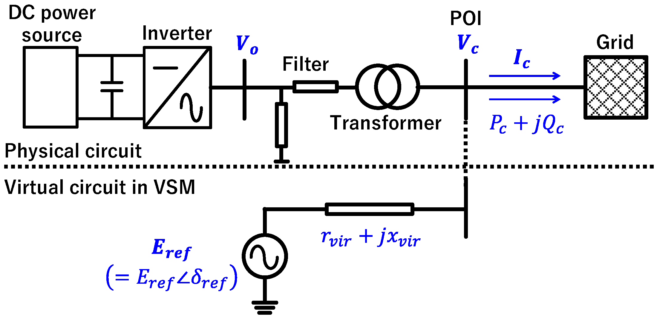
2.1. Virtual Synchronous Machine

As a manifestation of GFM virtual inertia control, this study targets a VSM [9,10,28]. A VSM is a method used to control an IBR by virtually simulating a synchronous generator inside the control system in such a way so that it appears from the power system side as though the generator is connected at the point of interconnection (POI) of the inverter. It is one of the most popular virtual inertia control schemes. Hereafter, the term ‘VI-GFM’ will be used to make it clear that it is a GFM-type VI control. Figure 1 shows a schematic of the VSM in application. The IBR, comprising a DC power source and an inverter, is connected to the power system via an output filter and a transformer. In the VSM, the output current $I_c$ is adjusted as if a virtually simulated synchronous generator (denoted as a voltage source in the figure) is connected at the POI via virtual impedance. This virtually simulated voltage source corresponds to the internal induced voltage of the synchronous generator. Hereafter, this will be referred to simply as the ‘internal voltage source’.

Figure 2 shows the VI-GFM control block diagram. The phase angle of the internal voltage source ${\delta }_{ref}$ is calculated as shown in Equations (1) and (2) based on the equation of motion of a synchronous generator.

$$M_G\frac{d{\omega }_{ref}\left(t\right)}{dt}=P_{ref}\left(t\right)-K_G\left\{{\omega }_{ref}\left(t\right)-{\omega }_0\right\}-P_C\left(t\right),$$

(1)

$$\frac{d{\delta }_{ref}\left(t\right)}{dt}={\omega }_{ref}\left(t\right),$$

(2)

Herein, $M_G$ is the inertia constant, $K_G$ is the control gain of the governor, $P_{ref}$ and $P_C$ are the active power reference and actual output, respectively, ${\omega }_{ref}$ and ${\delta }_{ref}$ are the references for angular frequency and phase angle of the internal voltage source, and ${\omega }_0$ is rated angular frequency. $P_C$ corresponds to the electric output of the synchronous generator, and $P_{ref}$ is equivalent to the reference value for mechanical input. The second term on the right side of the equation signifies the amount of adjustment of the mechanical input by the governor. With an ordinary synchronous generator, the response of the governor is delayed owing to the turbine and steam control valves, but in virtual inertia control, these mechanical restrictions can be omitted, and simulations conducted in the form of a simple droop mechanism are possible. The voltage magnitude of the internal voltage source $E_{ref}$ is determined by the AVR block so that the voltage at the POI $V_c$ follows the reference $V_{c,ref}^{\prime }$ through the integral controller with gain $K_c$. In the AVR, original voltage reference $V_{c,ref}$ is modified to the new reference $V_{c,ref}^{\prime }$ by the droop controller which with gain $K_{V,GFM}$, time delay $T_V$ according to difference in reactive power output $Q_c$ and its reference $Q_{ref}$.

The output current reference $I_{c,ref}$ is calculated based on Equation (3) using the internal source voltage $E_{ref}\left(=E_{ref}\angle {\delta }_{ref}\right)$ calculated as indicated above, the measured value of voltage at the POI $V_c$, and the virtual impedance $r_{vir}+j{x}_{vir}$.

$$I_{c,ref}=\frac{E_{ref}-V_c}{r_{vir}+j{x}_{vir}}$$

(3)

The current reference is calculated on the d–q coordinate axis. The voltage phase angle of the internal voltage source is used for the reference phase of Park’s transformation to project each variable onto the d–q coordinate axis. According to the calculated current reference, the output current of the IBR is adjusted by a general current control system [29]. The current control adjusts the inverter output voltage $V_o$ so that the d-axis and q-axis currents follow their respective reference values, and independent control on each axis is possible by decoupling. In conventional IBRs, the phase angle measured by a phase-locked loop (PLL) is used for the reference phase angle of Park’s transformation. However, in VI-GFM, there is phase angle information inside the control system; therefore, a characteristic of VI-GFM is that this information is used as the reference phase.

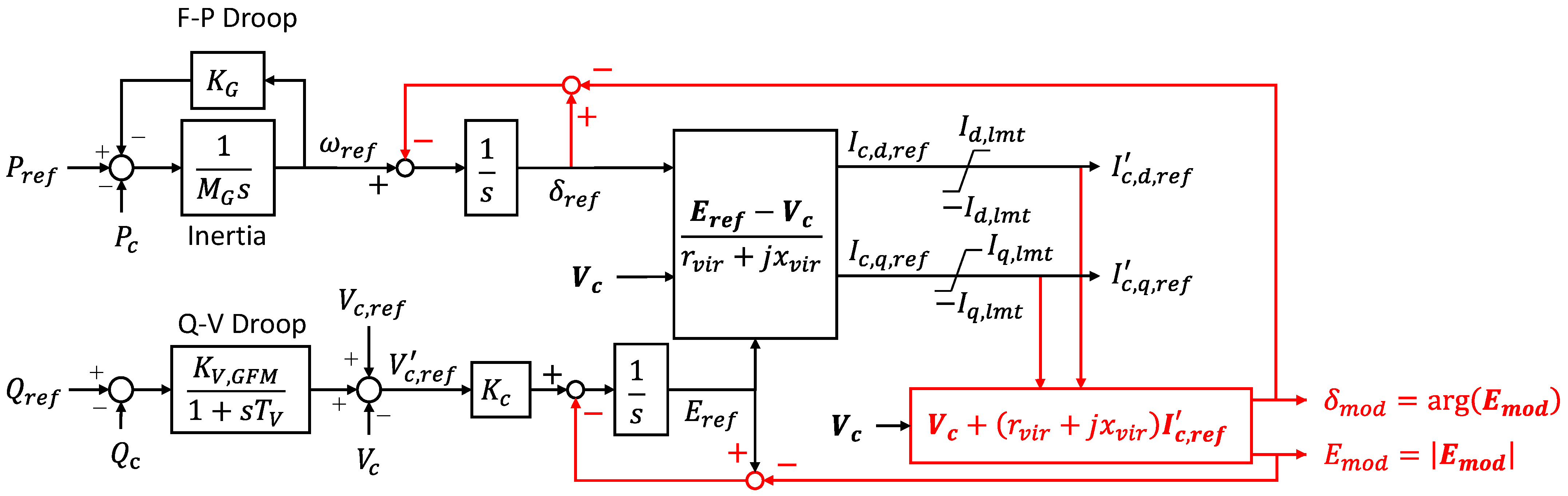
2.2. Proposed Modification Methodology

Because an IBR cannot output power in excess of the power from the DC side, it may not be possible to fully simulate the behavior of a large-capacity power source by virtual inertia control. In VI-GFM, current in excess of the capability of the IBR is prevented from being output by limiting the current reference value. There are two main methods used to limit the current. One method provides a saturation element in the current control reference value [18], and the other method suppresses the current reference value indirectly by temporarily increasing the virtual impedance [19,20,21,22,23,24,25]. The former method is used in this study.

When the current is suppressed, the output power to be fed back is suppressed, which affects the operation of the VSM. If the current required by the VSM is not output, the action of the synchronizing power will not be sufficient, the phase angle difference between the internal voltage source and the power system will increase, and the internal power source will fall out of synchronism. This study proposes a method to avoid the loss of synchronism by of modifying the voltage of the internal voltage source so that the synchronized state of the internal voltage source and the power system is not destroyed when the current is suppressed. Figure 3 shows the proposed control method. This method modifies the voltage of the internal voltage source to a value appropriate to the current which flows when the output current of the IBR is limited. Because the voltage of the internal voltage source is modified so that the limiting current flows, voltage divergence of the internal voltage source can be avoided. A saturation element is applied to the d- and q-axis current references, respectively, but it is necessary to ensure that the apparent current does not exceed the rated value. As shown by Equations (4) and (5), herein, a limitation is applied so that the norm becomes the limit value $I_{lmt}$ without changing the angle of the current vector. In the equations, $I_{d,lmt}$ and $I_{q,lmt}$ are the upper limits of the d- and q-axis currents, respectively.

$$I_{d,lmt}=I_{lmt} \cos \left\{{\tan }^{-1}\frac{I_{c,q,ref}}{I_{c,d,ref}}\right\}$$

(4)

$$I_{q,lmt}=\sqrt{I_{lmt}^2-I_{d,lmt}^2}$$

(5)

If the current reference changes owing to this limitation, the relationship in Equation (3) will no longer hold true and the substantial voltage of the internal voltage source will not be $E_{ref}$. Assuming that the substantial voltage of the internal voltage source is $E_{mod}$, $E_{mod}$ can be calculated by using Equation (6).

$$E_{mod}=V_c+\left(r_{vir}+j{x}_{vir}\right)I_{c,ref}^{\prime }$$

(6)

By performing anti-windup control so that the voltage reference of the internal voltage source becomes the modified voltage, extreme fluctuation in the phase angle of the internal voltage source is suppressed and loss of synchronism can be prevented. Various methods of limiting current and their effects on stability have been studied, but there are no examples of studies on methods that modify the reference values of virtual inertia control according to the current limitation. This constitutes the major novelty of this study. In steady state, which means that the current is not limited, the proposed method does not affect on the internal induced voltage. Because (6) is the inverse function of (3), $E_{mod}$ equals to $E_{ref}$ if the current is not limited. This is also an advantage of the proposal.

3. Simulation Model and Condition

A simulation study was conducted to evaluate the difference in the behavior of the VI-GFM depending on the presence or absence of the proposed modification logic for the voltage of the internal voltage source, and to evaluate the effect of current limitation on frequency stability after implementing the proposed method. In the evaluation of the effect on frequency stability, GFL-type virtual inertia control was also studied, and the question of how the effect of current limitation differs between GFM and GFL was evaluated.

Three types of simulations were performed in this study. First, in Step 1, the frequency stability of a power system was evaluated in which the power sources were synchronous generators only and no IBRs were installed, based on the consideration of the power source trip as a disturbance. In Step 2, a case in which a conventional IBR with a fixed output was installed was analyzed. These two simulations are reference cases used for the evaluation of the effects of the installation of an IBR that implements virtual inertia control. Finally, in Step 3, a case in which an IBR with virtual inertia control is installed was examined. Herein, differences in the behavior of the VI-GFM depending on the presence or absence of the proposed logic and the effect of current limitation on frequency stability were evaluated. The effect of current limitation was examined in a similar manner for GFL-type virtual inertia control, and a comparative study of GFL and GFM was conducted.

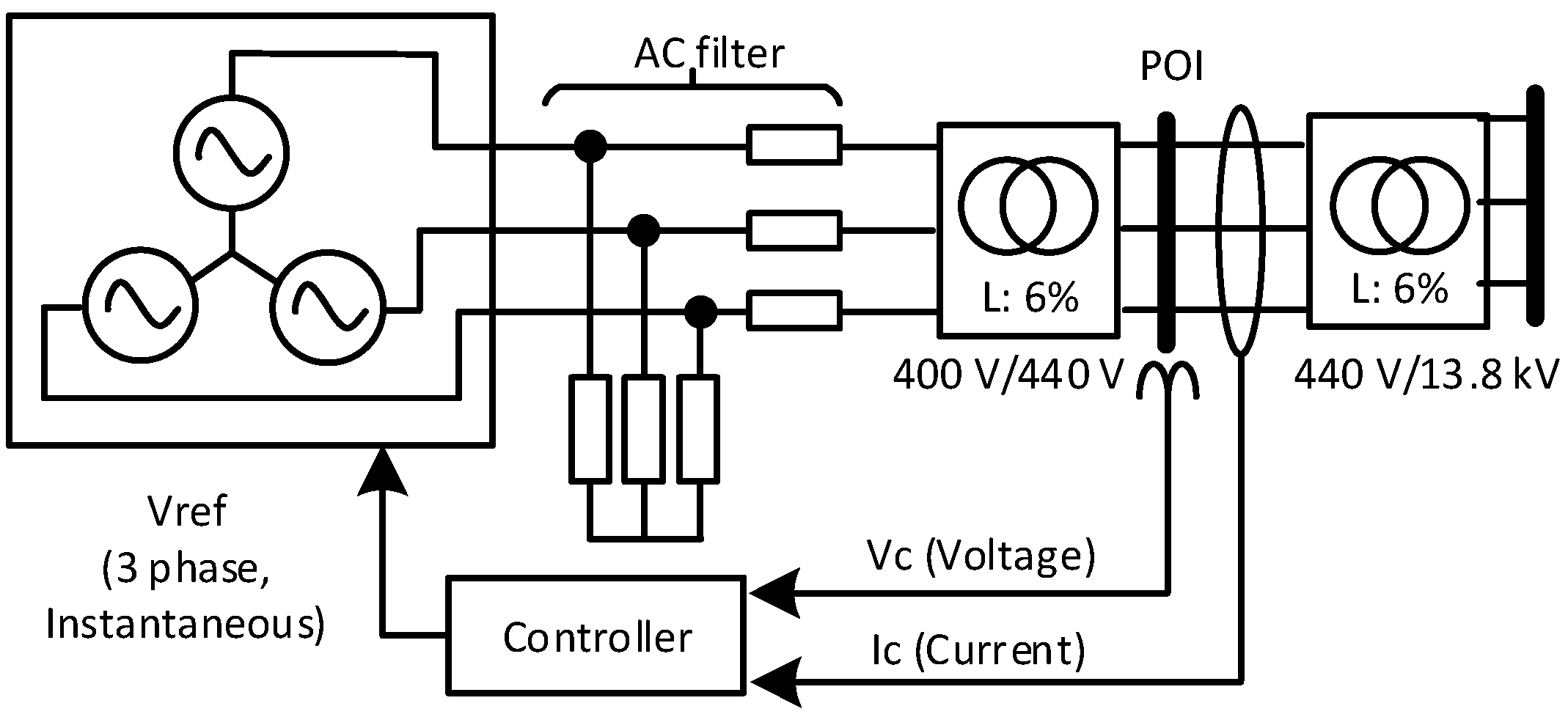
3.1. Power System Model

In this study, the power system model based on the Institution of Electrical and Electronic Engineers (IEEE) nine-bus system [30] was used, as shown in Figure 4. The power sources consist of S1, S2, S3, and SD. In Step 1, they are all synchronous generators, but in Steps 2 and 3, power source S3 is replaced with an IBR. Power source SD is a small-scale power source used to simulate a disturbance. The synchronous generator model is the sixth-order Park’s model, and a governor, turbine, and a AVR with a PSS are modeled [31] as controllers. The average model is used for the IBR. As shown in Figure 5, this modeling method implements the voltage reference values generated by the inverter control system directly by using an AC voltage source. Because switching is not simulated, harmonics do not appear and only fundamental waves can be analyzed, but the calculation accuracy of the fundamental wave components is high, and the computation load can be reduced considerably [32]. In this study, the DC-side circuit was not simulated. Changes in the available output power of the power source on the DC side were simulated based on the changes in the upper limit of the current in the current control.

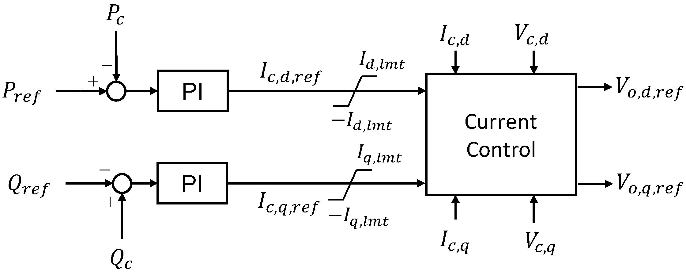
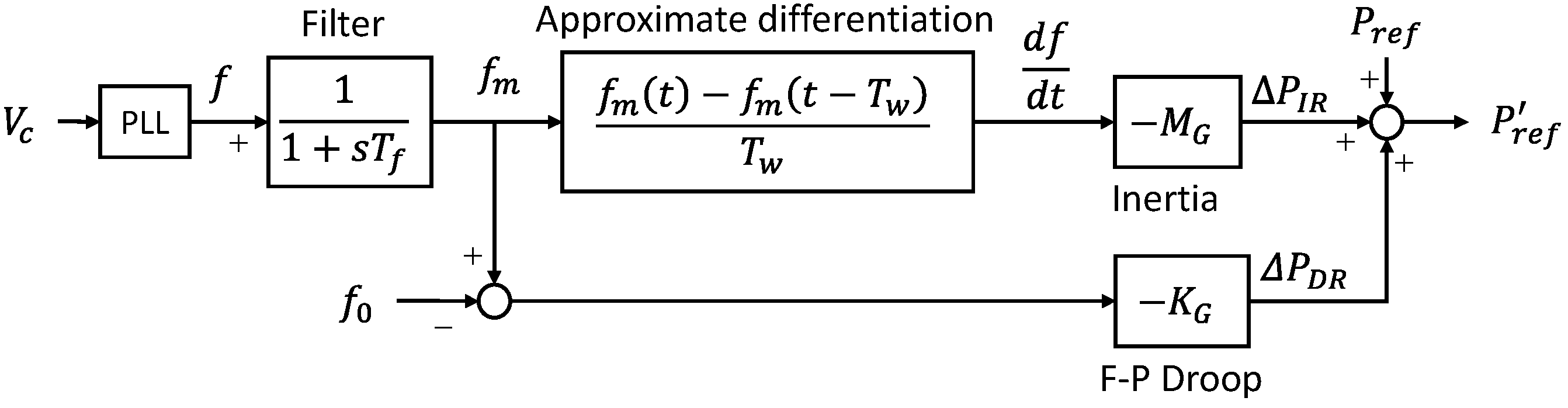
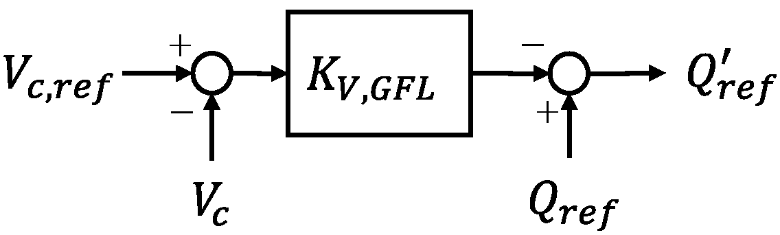
3.2. IBR Model for Comparison Study

In this simulation study, in addition to VI-GFM, conventional control and GFL-type virtual inertia control were also analyzed for comparison. This section describes these models. First, Figure 6 shows a block diagram of the conventional control. The current control section is common with the VI-GFM, and the d- and q-axis current reference values are adjusted by active and reactive power control, respectively. In solar and wind power generation, the maximum available generation power—which varies depending on the weather conditions—is input as an active power reference value. However, in this study, the analysis was performed based on the assumption that the active power reference value is constant to focus on phenomena in the first few seconds after generator trip. Additionally, taking the reactive power reference value as zero, the condition of operating always at a power factor of 1 was set. The voltage phase angle at the POI measured by a PLL was used for the reference phase of Park’s transformation.

Figure 7 shows a block diagram of the GFL-type virtual inertia control. Hereafter, this control method will be referred to as ‘VI-GFL’. The left side of Equation (1) means that the power goes in and out of the rotor of the synchronous generator, which means the inertial response. By calculating the power corresponding to the left side of Equation (1) from the measured frequency value, it is possible to simulate the inertial response of the synchronous generator, which is output or absorbed from the IBR. The derivative of the frequency is pseudo-computed as a slope of frequency with time window of $T_W$. It, along with the PLL measured frequency $f$, is filtered by low-pass filter (LPF) with time constant $T_f$. The frequency $f_m$ is the output of the LPF and used for the slope computation. In VI-GFL, as in VI-GFM, a function used to adjust the active power in proportion to the frequency was provided to simulate the governor’s response. Additionally, to achieve voltage control by reactive power adjustment appropriate for VI-GFL, a voltage control function with droop characteristics was modeled as shown in Figure 8. By assigning the droop gain so that it is inversely related to the droop gain in the AVR of the VI-GFM, the relationship between voltage and reactive power can be equated. Regarding the current limitation in the VI-GFL, only a saturation element in the current control reference value was provided. This is because, unlike VI-GFM, VI-GFL does not have internal phase information, and destabilization similar to loss of synchronism does not occur.

3.3. Simulation Condition

We evaluated two subjects through the simulation study. One was an evaluation of the effectiveness of the proposed method that identified whether destabilization can be prevented by modifying the voltage of the internal voltage source in VI-GFM. The other was an evaluation of the effect of limiting the response of the simulated inertia control on frequency stability by limiting current. The effect was analyzed in detail by taking the penetration rate of IBRs and the value of the upper limit of current limitation as parameters.

Table 1. Indices of the simulation study.

Step	Source Connected as S3	S3 Capacity Ratio Corresponding to IBR 1 Penetration Rate in Steps 2 and 3
		20% (Low)	60% (High)
1	Synchronous generator	#1-L	#1-H
2	IBR 1: conventional control	#2-L	#2-H
3	IBR 1: VI-GFM 2 without proposed modification logic	#3-GFM-L	#3-GFM-H
	IBR 1: VI-GFM 2 with proposed modification logic	#3-GFMpro-L	#3-GFMpro-H
	IBR 1: VI-GFL 3	#3-GFL-L	#3-GFL-H

¹ Inverter-based resource (IBR), ² grid-forming virtual inertia control (VI-GFM), ³ grid-following virtual inertia control (VI-GFL).

shows the case indices according to the analysis condition. Cases in which the IBR penetration rate was 20% and 60% of the power system capacity were considered. Analyses of steps 1, 2, and 3 were conducted for each penetration rate. For Step 3, three types of control were evaluated separately: VI-GFM with the proposed logic, VI-GFM without the proposed logic, and VI-GFL. In Step 1, as no IBR was included, the capacity of the synchronous generator connected as the power source S3 was changed. The rated capacities of power sources S1 and S2 were also changed as shown in

Table 2. Rated capacities of the generation units at each IBR penetration rate.

Percentage of S3 Capacity 1 (Means IBR Penetration Rate in Steps 2 and 3)	Rated Capacity (MVA)
	S1 (SG 2)	S2 (SG 2)	S3 (Step 1: SG 2, Step 2, 3: IBR)
20%	120	120	60
60%	60	60	180

¹ SD is not considered in the percentage. The capacity of SD is 10 MVA in all cases. ² SG denotes the synchronous generator.

so that the system capacity was fixed even when the IBR penetration rate was changed. The capacity of the power source SD was maintained constant so that the size of the disturbance was constant. For each case in Table 1, multiple cases with different current limitation values were analyzed. The current limitation settings were determined based on the results of a base-case simulation in which current limitation was not used. The details are presented in the next section.

The demand settings were common to all cases, and the active power demand for a power system capacity of 300 MVA was set to 80% (240 MW), equally distributed among three load buses. For reactive power demand, the power factor of each bus in the IEEE nine-bus system was set. Additionally, the output distribution in the initial state of each power source was taken to be the rated capacity ratio of the power source. In this simulation, the disturbance is the disconnection of the power source SD. The rated capacity of SD was 10 MVA, and its output was 5 MW. It was disconnected at 80 s.

Table 3. Control parameters of IBR.

Algorithm	Control Parameter	Letter	Value
VI-GFM, VI-GFL (common)	Inertia constant	$M_G$	4.70 (s)
	Governor gain	$K_G$	25.0
VI-GFL	Voltage control gain	$K_{V,GFL}$	10.0
	Time constant of low-pass filter	$T_f$	0.10 (s)
	Time window of the slope computation	$T_W$	0.10 (s)
VI-GFM	Voltage control gain	$K_{V,GFM}$	0.10
	Time constant of voltage controller	$T_V$	0.02 (s)

shows the control parameters assigned to controllers of VI-GFM, VI-GFL. The inertia constant $M_G$ and the governor control gain $K_G$ are set to be the same as the power source S3 in IEEE nine-bus system. The voltage control gains in VI-GFM and VI-GFL are set to be inverse values to have equivalent capability in voltage regulation. Time constants are determined by trial-and-error so that the stable operation is ensured as much as possible.

4. Results

First, Section 4.1 explains the results of the base-case simulation to determine the current limitation settings. Section 4.2 explains the results of the evaluation of effectiveness of the proposed modification logic of the voltage of the internal voltage source in the VI-GFM. Finally, Section 4.3 explains the results of evaluating the relationship between the current limitation value and frequency stability.

4.1. Base-Case Simulation to Set Simulation Conditions

In this study, the effects on the performance of virtual inertia control in multiple cases with different current limitation settings were analyzed. The current limitation settings were determined as follows based on the results of a base-case simulation without current limitation elements. Figure 9 shows the IBR output current when VI-GFM and VI-GFL were used at each IBR penetration rate. For the VI-GFM, the model did not implement the proposed modification logic. The figure shows that the current is temporarily increased in response to the power source trip, and eventually converges to a state in which part of the power loss is shared. The maximum current value and final current value (value at a time of 120 s) are shown in the figure.

Table 4. Current limitation settings.

Case Index	IBR Penetration Ratio
	20%		60%
	VI-GFM	VI-GFL	VI-GFM	VI-GFL
No limit case	1.20 pu	1.20 pu	1.20 pu	1.20 pu
90% case	0.832 pu	0.832 pu	0.817 pu	0.818 pu
80% case	0.828 pu	0.828 pu	0.814 pu	0.815 pu
70% case	0.824 pu	0.824 pu	-	0.813 pu
60% case	0.820 pu	0.820 pu	-	-
50% case	0.816 pu	0.816 pu	-	-

shows the current limitation settings determined based on this result. Taking the difference between the current value before the disturbance occurrence and the maximum value as 100%, the upper current limit was set to decrease at 10% intervals given that the setting was not set lower than the final value. This is because a situation was assumed in which there was enough extra power only for the power borne by the IBR after convergence. The aim of the study was to evaluate the effect when a transient response for several seconds after power source trip was limited. In the case of an IBR penetration rate of 60%, the transient fluctuation was relatively small, and there were few verifiable current limitation settings.

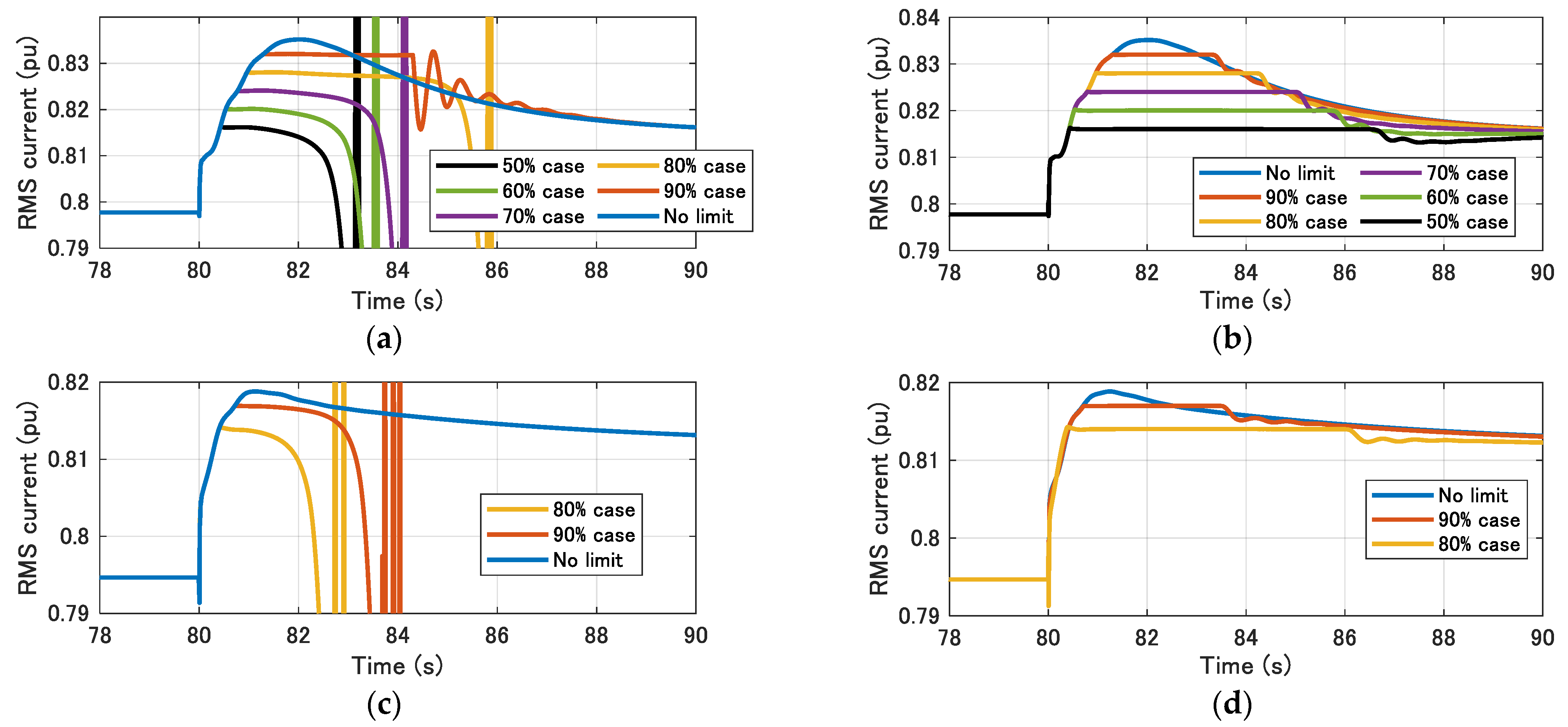
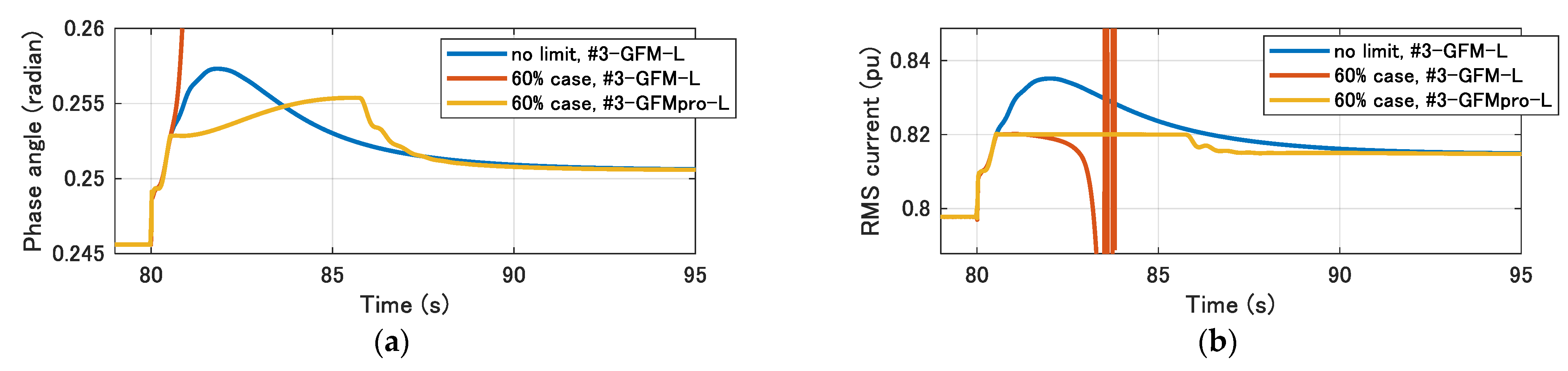
4.2. Effectiveness of Proposed Methodology

This section verifies the effectiveness of the proposed modification logic of the internal voltage source in the VI-GFM. Figure 10 shows the IBR output current as a function of the IBR penetration rate when the proposed method was/was not applied. The figure shows that regardless of whether the proposed method was applied, the increase in the current immediately after the disturbance was suppressed by the current limitation. However, when the proposed method was not applied, in most cases, several seconds after reaching the upper limit, the current suddenly decreased and oscillated persistently, as indicated in Figure 10a,c. Herein, if an undamped oscillation occurred, the data plotting in the figure was stopped a few moments after the oscillation, to ensure visibility. In the #3-GFM-L 90% case, continuous oscillation did not occur, but at 84 s, when the current was no longer limited, small vibration was observed. The figure also shows that as the upper limit was lowered, the oscillation was reached earlier. Meanwhile, Figure 10b,d shows that destabilization is avoided by using the proposed modification logic, regardless of the current upper limit, which demonstrates the effectiveness of the proposed method.

In the rest of this section, the mechanism of the destabilization of the VI-GFM seen in Figure 10a,c is considered according to the behavior of the internal induced voltage, and the reason why it is improved by the proposed method is also considered. Figure 11a,b respectively show the phase angle of the voltage of the internal voltage source in VI-GFM in terms of system voltage and the output current of the IBR in #3-GFM-L (no limit case), #3-GFM-L (60% case), #3-GFMpro-L (60% case). The figures show that the phase angle increases after the generator trip in the same way as in all cases until 80.5 s when the current reach its limitation. After that, in #3-GFM-L (60% case), the phase angle increased to a large degree and diverged. It is expected that enough synchronizing power for deacceleration of the simulated synchronous generator was not supplied because the current limitation suppressed active power output of the IBR. This corresponds to the loss of synchronism among synchronous generators. The arguments listed above show that by simply applying a saturation element in current control, destabilization of control occurs due to phase angle divergence of the internal voltage source.

On the other hand, in #3-GFMpro-L (60% case) in which the proposed method was applied, when the current reached the limit value, the increase in the phase angle of the internal voltage source became gradual, and this did not lead to divergence. While the current stays at the upper limit, the active power output does not increase even if the phase angle of the internal voltage source increases unlike synchronous generator. In such a condition, the proposed method suppresses the phase angle increase so that the Kirchhoff’s law is satisfied and maintains the synchronization of the internal voltage source and the grid. When the current reference was released from the upper limit at 86 s, VI-GFM with the proposed method seamlessly returned to the normal operation in which the phase angle was not modified.

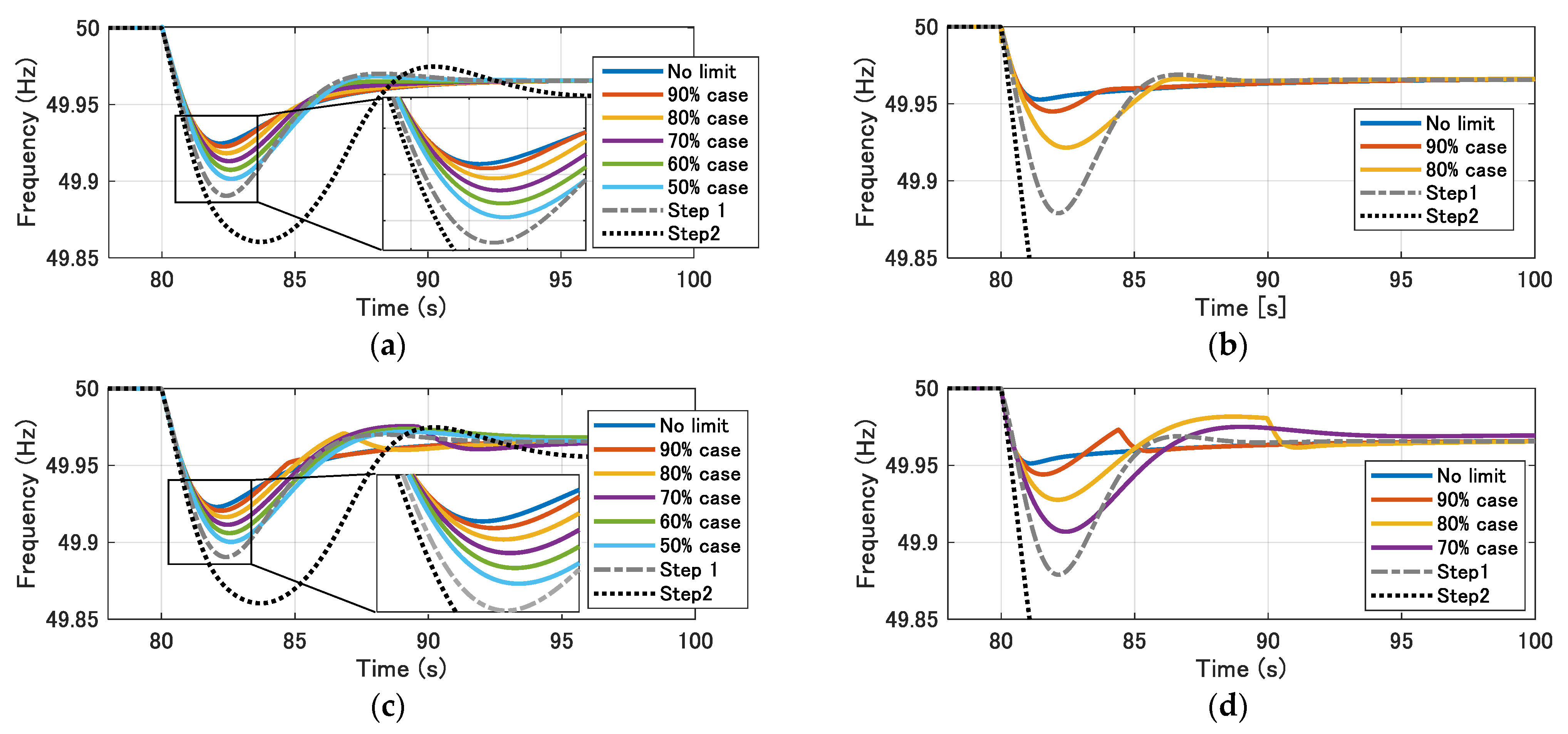
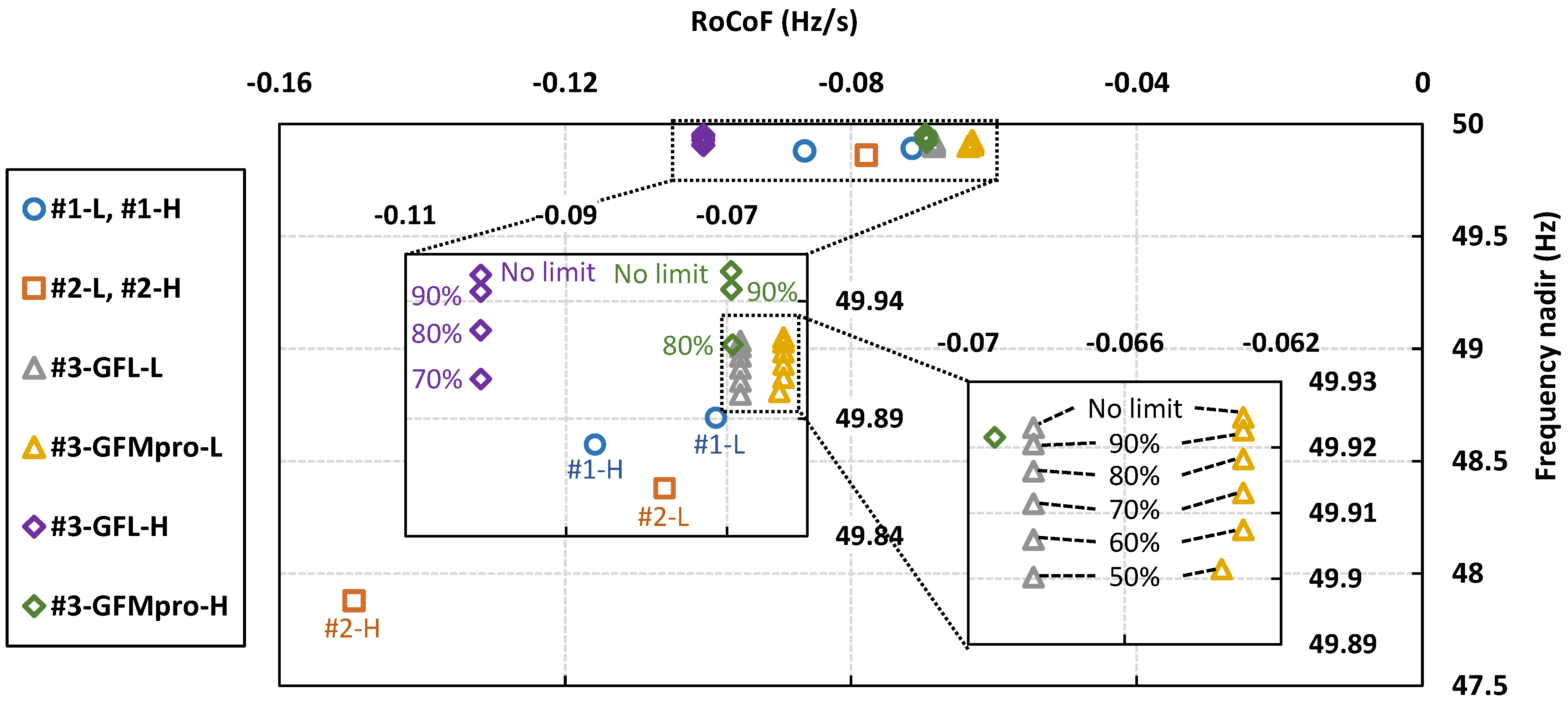
4.3. Frequency Stability Evaluation

This section explains the results of the evaluation of the effect of limiting the output response of virtual inertia control by current limitation on frequency stability. Figure 12a–d shows the calculation results for center of inertia frequency in #3-GFMpro-L, #3-GFMpro-H, #3-GFL-L, and #3-GFL-H, respectively. For comparison, the figures also show the simulation results for Steps 1 and 2 which correspond to each case. Herein, the center of inertia (COI) frequency is the average frequency of the entire system based on considerations of the difference in inertia between generators, and it is calculated using the following equation. In power systems with multiple generators, this is used to monitor the average frequency of the entire system without the effect of oscillations between generators [33].

$$f_{COI}\left(t\right)=\frac{{{\displaystyle \sum }}_{i=1}^{N_G}{M}_i{f}_i\left(t\right)}{{{\displaystyle \sum }}_{i=1}^{N_G}{M}_i}$$

(7)

In Figure 12a, frequency fluctuation was greater in Step 2 than in Step 1. This is because system inertia and frequency control capability of the governor were reduced owing to the fact that the synchronous machine of S3 was replaced with a conventional IBR. However, in #3-GFMpro-L (no limit), in which the current limitation setting was sufficiently large, frequency fluctuation was reduced considerably compared with Step 1. This was mainly attributed to primary control capability of the synchronous machine and the VI-GFM. In a synchronous machine, because the governor and turbine have a mechanical response delay, it takes a few seconds for the primary control reserve to exert an effect; by contrast in VI-GFM, it is possible to obtain a response without any delay. As a result, the IBR can respond quickly to a disturbance, thus reducing the burden on other synchronous machines, and thus suppressing frequency fluctuations. When the current limitation setting was decreased, the burden on the other synchronous machines and frequency fluctuations increased owing to the limited transient response of the IBR. However, even in #3-GFMpro-L (50% case), which had the lowest limit value, the maximum deviation of frequency fluctuation was comparable to #1-L, that is, the frequency fluctuation was not worse than in the conventional synchronous machine system. This means that the disadvantage of the suppression of the IBR output changes was accounted for by the readiness of the governor control. A similar trend can be confirmed in the other cases shown in Figure 12b–d. Collectively, the arguments listed above show that although maximum frequency deviation increases owing to the limitations of the transient response by the current limitation, if the control reserve required for load sharing after convergence is secured, it is possible to maintain the frequency fluctuation to the level of a conventional synchronous machine system.

The frequency fluctuation was then converted to index values in each case, and a quantitative comparison was performed. The frequency nadir, which is the minimum value of the COI frequency, and rate-of-change of frequency (RoCoF), which is the minimum rate of change of the COI frequency, were then used. Equations (8) and (9) show the definition of RoCoF. Herein, the minimum rate of change calculated from the frequencies observed in interval $T_s$ (seconds) is denoted by RoCoF. RoCoF is calculated was limited to the range from the disturbance occurrence until the appearance of the frequency nadir at time $t_{nadir}$. In this evaluation, $T_s$ was set to 100 ms.

$$RoCoF=\underset{i=1, 2, \cdots , K }{\min }\frac{f_{COI}\left(t_0+i{T}_s\right)-f_{COI}\left(t_0+\left(i-1\right)T_s\right)}{T_s}$$

(8)

$$K=\max \left\{n\in \mathbb{Z}|n\le \frac{t_{nadir}-t_0}{T_s}\right\}$$

(9)

Figure 13 shows the correlation between RoCoF and the frequency nadir. After the disturbance occurred, frequency continued to decrease until the frequency nadir appeared. Therefore, RoCoF took a negative value. As the value of RoCoF increased, the change in frequency became more gradual. Additionally, as the frequency nadir increased, the magnitude of the frequency fluctuation became smaller. First, the results associated with the comparison of Steps 1 and 2 show that RoCoF and the frequency nadir were both worse in Step 2 compared with Step 1, regardless of the IBR penetration rate. This is due to a reduction in inertia and a reduction in frequency control capability of the governor owing to a decrease in the number of synchronous generators. In Step 3, in VI-GFM (#3-GFMpro-L, #3-GFMpro-H), both RoCoF and the frequency nadir were larger than those in Step 1, regardless of IBR penetration rate and current limitation setting. As mentioned previously, this is due to the fast governor response. In VI-GFM, because the governor response is extremely fast compared with the synchronous machine, the effect is observed at the frequency nadir, which appears within a few seconds after the disturbance, and at the RoCoF, which appears within a few hundred milliseconds after the disturbance. Regarding the subject of this study, which is the effect of current limitation, the results show that regardless of IBR penetration rate, as the current limitation setting decreases, the frequency nadir worsens, but RoCoF does not worsen. This is because, as shown in Figure 10, there is a small period between the occurring of the disturbance and the current limitation. In many cases, the RoCoF appears during this period, specifically between 200 ms and 300 ms after the disturbance. However, if the current limitation setting decreases, the current is affected by the current limitation sooner, and it is therefore possible that RoCoF will worsen, albeit slightly, as in the #3-GFMpro-L 50% case.

In VI-GFL (#3-GFL-L, #3-GFL-H), although the results are broadly similar to VI-GFM, in #3-GFL-H with a high IBR penetration rate, RoCoF was worse compared with Step 1. This is attributed to the low responsiveness of VI-GFL. Because output references are determined from the frequency measured by a PLL, the VI-GFL is affected by the measurement delay of the PLL. However, an improvement effect is observed compared with Step 2. Additionally, because the PLL operation is stable in the time domain of the governor’s response, the improvement effect on the frequency nadir is approximately the same as that of the VI-GFM. The effect of current limitation was similar to the VI-GFM with no current limitation effects on RoCoF.

5. Conclusions

Virtual inertia control using IBRs is expected to be an effective measure against low inertia. However, the control response may be limited by the maximum output of the power source on the DC side and the inverter capacity, thus resulting in performance deterioration. This study showed that current limitation causes grid-forming virtual inertia control (VI-GFM) to be unable to provide synchronizing power, thus causing instability of control comparable to a loss of synchronism. We proposed a to modify the internal induced voltage of the simulated synchronous generator inside the control system of the inverter according to the output current. A simulation study showed that it is possible to prevent instability of the voltage phase angle of the VI-GFM by applying the proposed method.

Additionally, simulations were used to evaluate the influence of the suppression of the output response by current limitation on frequency stability in VI-GFM with the proposed method applied and grid-following virtual inertia control (VI-GFL). The results showed that because there is a small amount of time between the occurrence of the disturbance and the limitation of the current, the influence of current limitation on the most rapid frequency changes that appeared immediately after the disturbance were small. Additionally, as the current limitation setting was lowered, the maximum frequency deviation which appeared a few seconds after the disturbance became greater. However, it was also found that if the IBR had a sufficient generation margin to meet the load shared by the control reserve for governor, even if it was affected transiently by current limitations, the frequency fluctuation will not become worse compared with a synchronous machine system without IBRs. This finding has important implications pertaining to the extent of control reserve IBRs should possess to perform virtual inertia control.

The proposed method can avoid the instability of the VI-GFM caused by current limitation. However, while the current is held to the limit, the VI-GFM cannot provide any more inertial response nor supply synchronizing power. This is a limitation of the proposed method. The influence of the limitation on the frequency stability is discussed in this paper, but it also affects the stability of synchronization of so called phase angle stability. The effect of the proposed method on the phase angle stability needs to be evaluated quantitively in the future. Eventually, we will extract the requirements for the IBR for its contribution to enhancement of the system stability from our and relevant research and those are organized for standardization.

References

1. Electric Power Research Institute. Basic Classification of Inverters; Technical Update; Electric Power Research Insititute: Palo Alto, CA, USA, 2019. [Google Scholar]
2. Lin, Y.; Eto, J.H.; Johnson, B.B.; Flicker, J.D.; Lasseter, R.H.; Pico, H.N.V.; Seo, G.; Pierre, B.J.; Ellis, A. Research Roadmap on Grid-Forming Inverters; NREL Technical Report for National Renewable Energy Lab: Golden, CO, USA, 2020. [Google Scholar]
3. Matevosyan, J.; Badrzadeh, B.; Prevost, T.; Quitmann, E.; Ramasubramanian, D.; Urdal, H.; Huang, S.H.; Vital, V.; O’Sullivan, J.; Quint, R. Grid-forming inverters: Are they the key for high renewable penetration? IEEE Power Energy Mag. 2019, 17, 89–98. [Google Scholar] [CrossRef]
4. Gui, Y.; Wang, X.; Blaabjerg, F.; Pan, D. Control of grid-connected voltage-source converters: The relationship between direct-power control and vector-current control. IEEE Ind. Electron. Mag. 2019, 13, 31–40. [Google Scholar] [CrossRef] [Green Version]
5. Kroposki, B.; Johnson, B.; Zhang, Y.; Gevorgian, V.; Denholm, P.; Hodge, B.; Hannegan, B. Achieving a 100% renewable grid: Operating electric power systems with extremely high levels of variable renewable energy. IEEE Power Energy Mag. 2017, 15, 61–73. [Google Scholar] [CrossRef]
6. Yap, K.Y.; Charles, C.R.; Lim, J.M.-Y. Virtual inertia-based inverters for mitigating frequency instability in grid-connected renewable energy system: A review. Appl. Sci. 2019, 9, 5300. [Google Scholar] [CrossRef] [Green Version]
7. Unruh, P.; Nuschke, M.; Strauß, P.; Welck, F. Overview on grid-forming inverter control methods. Energies 2020, 13, 2589. [Google Scholar] [CrossRef]
8. Tamrakar, U.; Shrestha, D.; Maharjan, M.; Bhattarai, B.P.; Hansen, T.M.; Tonkoski, R. Virtual inertia: Current trends and future firections. Appl. Sci. 2017, 7, 654. [Google Scholar] [CrossRef]
9. Electric Power Research Institute. Grid Forming Inverters; EPRI Tutorial; Electric Power Research Insititute: Palo Alto, CA, USA, 2021. [Google Scholar]
10. Paolone, M.; Gaunt, T.; Guillaud, X.; Liserre, M.; Meliopoulos, S.; Monti, A.; van Cutsem, T.; Vittal, V.; Vournas, C. Fundamentals of power systems modelling in the presence of converter-interfaced generation. Electr. Power Syst. Res. 2020, 189, 106811. [Google Scholar] [CrossRef]
11. Elkhatib, M.E.; Du, W.; Lasseter, R.H. Evaluation of Inverter-based Grid Frequency Support using Frequency-Watt and Grid-Forming PV Inverters. In Proceedings of the 2018 IEEE Power & Energy Society General Meeting (PESGM), Portland, OR, USA, 5–10 August 2018; pp. 1–5. [Google Scholar]
12. Pattabiraman, D.; Lasseter, R.H.; Jahns, T.M. Comparison of Grid Following and Grid Forming Control for a High Inverter Penetration Power System. In Proceedings of the 2018 IEEE Power & Energy Society General Meeting (PESGM), Portland, OR, USA, 5–10 August 2018; pp. 1–5. [Google Scholar]
13. Liu, J.; Miura, Y.; Ise, T. Comparison of dynamic characteristics between virtual synchronous generator and droop control in inverter-based distributed generators. IEEE Trans. Power Electron. 2016, 31, 3600–3611. [Google Scholar] [CrossRef]
14. Qoria, T.; Gruson, F.; Colas, F.; Denis, G.; Prevost, T.; Guiillaud, X. Critical clearing time determination and enhancement of grid-forming converters embedding virtual impedance as current limitation algorithm. IEEE J. Emerg. Sel. Top. Power Electron. 2020, 8, 1050–1061. [Google Scholar] [CrossRef] [Green Version]
15. Qoria, T.; Gruson, F.; Colas, F.; Kestelyn, X.; Guillaud, X. Current Limiting Algorithms and Transient Stability Analysis of Grid-Forming VSCs. Electr. Power Syst. Res. 2020, 189, 106726. [Google Scholar] [CrossRef]
16. Samanta, S.; Chaudhuri, N.R. On Stability Analysis of Power Grids with Synchronous Generators and Grid-Forming Converters under DC-side Current Limitation. In Proceedings of the IEEE 2021 American Control Conference (ACC), Online Conference, 25–28 May 2021; pp. 1817–1823. [Google Scholar]
17. Zhou, L.; Liu, S.; Chen, Y.; Yi, W.; Wang, S.; Zhou, X.; Wu, W.; Zhou, J.; Xiao, C.; Liu, A. Harmonic Current and Inrush Fault Current Coordinated Suppression Method for VSG Under Non-ideal Grid Condition. IEEE Trans. Power Electron. 2021, 36, 1030–1042. [Google Scholar] [CrossRef]
18. Narita, T.; Sugimori, S.; Nakajima, T.; Mitsugu, Y.; Hashiguchi, H. Overcurrent Suppression Control for Grid Forming Inverter. In Proceedings of the 11th Solar & Storage Power System Integration Workshop, Berlin, Germany, 28 September 2021. [Google Scholar]
19. He, J.; Wei, Y. Analysis, design, and implementation of virtual impedance for power electronics interfaced distributed generation. IEEE Trans. Ind. Appl. 2011, 47, 2525–2538. [Google Scholar] [CrossRef]
20. Beheshtaein, D.; Golestan, S.; Cuzner, R.; Guerrero, J.M. A New Adaptive Virtual Impedance based Fault Current Limiter for Converters. In Proceedings of the 2019 IEEE Energy Conversion Congress and Exposition (ECCE), Baltimore, MD, USA, 29 September–3 October 2019; pp. 2439–2444. [Google Scholar]
21. Yan, J.; Zhao, C.; Zhang, F.; Xu, J. The preemptive virtual impedance based fault current limiting control for MMC-HVDC. In Proceedings of the 8th Renewable Power Generation Conference (RPG 2019), Shanghai, China, 24–25 October 2019; pp. 1–6. [Google Scholar]
22. Lin, X.; Liang, Z.; Zheng, Y.; Lin, Y.; Kang, Y. A current limiting strategy with parallel virtual impedance for three-phase three-leg inverter under asymmetrical short-circuit fault to improve the controllable capability of fault currents. IEEE Trans. Power Electron. 2019, 34, 8138–8149. [Google Scholar] [CrossRef]
23. Zhao, X.; Flynn, D. Freezing Grid-Forming Converter Virtual Angular Speed to Enhance Transient Stability Under Current Reference Limiting. In Proceedings of the 2020 IEEE 21st Workshop on Control and Modeling for Power Electronics (COMPEL), Aalborg, Denmark, 9–12 November 2020; pp. 1–7. [Google Scholar]
24. Paquette, A.D.; Divan, D.M. Virtual impedance current limiting for inverters in microgrids with synchronous generators. IEEE Trans. Ind. Appl. 2015, 51, 1630–1638. [Google Scholar] [CrossRef]
25. Groß, D.; Dörfler, F. Projected Grid-forming Control for Current-limiting of Power Converters. In Proceedings of the 2019 57th Annual Allerton Conference on Communication, Control, and Computing (Allerton), Monticello, IL, USA, 24–27 September 2019; p. 326333. [Google Scholar]
26. Pattabiraman, D.; Lasseter, R.H.; Jahns, T.M. Transient Stability Modeling of Droop-Controlled Grid-Forming Inverters with Fault Current Limiting. In Proceedings of the 2020 IEEE Power & Energy Society General Meeting (PESGM), Montreal, QC, Canada, 2–6 August 2020; pp. 1–5. [Google Scholar]
27. Li, Y.; Meng, K.; Dong, Z.Y. Frequency Enhancement of Grid-forming Inverters under Low-SCR Weak Grid. In Proceedings of the 8th Renewable Power Generation Conference (RPG 2019), Shanghai, China, 24–25 October 2019; pp. 1–7. [Google Scholar]
28. Hirase, Y.; Uezaki, K.; Orihara, D.; Kikusato, H.; Hashimoto, J. Characteristic analysis and indexing of multimachine transient stabilization using virtual synchronous generator control. Energies 2021, 14, 366. [Google Scholar] [CrossRef]
29. Rowan, T.M.; Kerkman, R.J. A new synchronous current regulator and an analysis of current-regulated PWM inverters. IEEE Trans. Ind. Appl. 1986, IA-22, 678–690. [Google Scholar] [CrossRef]
30. Anderson, P.M.; Fouad, A.A. Power System Control and Stability, 2nd ed.; IEEE Press: Piscataway, NJ, USA, 2003; pp. 13–52, 83–148. [Google Scholar]
31. Orihara, D.; Kikusato, H.; Hashimoto, J.; Otani, K.; Takamatsu, T.; Oozeki, T.; Taoka, H.; Matsuura, T.; Miyazaki, S.; Hamada, H.; et al. Contribution of voltage support function to virtual inertia control performance of inverter-based resource in frequency stability. Energies 2021, 14, 4220. [Google Scholar] [CrossRef]
32. Mo, O. Average Model of PWM Converter; Project memo AN 03.12.103; SINTEF Energy Research: Trondheim, Norway, 2003. [Google Scholar]
33. Kundur, P. Power System Stability and Control; McGraw-Hill: New York, NY, USA, 1994. [Google Scholar]
Figure 1. Physical configuration of inverter-based resource (IBR) interconnection and simulated virtual connection configuration in virtual synchronous machine (VSM), grid-forming virtual inertia control (VI-GFM).
Energies 15 00901 g001
Figure 2. Block diagram of controller of VI-GFM.
Energies 15 00901 g002
Figure 3. Current limitation with the proposed method modifying internal induced voltage of synchronous generator virtually simulated inside VI-GFM.
Energies 15 00901 g003
Figure 4. Power system model [31].
Energies 15 00901 g004
Figure 5. Average IBR model [31].
Energies 15 00901 g005
Figure 6. Controller model of the conventional IBR used in the simulation in Step 2.
Energies 15 00901 g006
Figure 7. Controller model of the grid-following virtual inertia control (VI-GFL) used in a part of the simulation in Step 3.
Energies 15 00901 g007
Figure 8. Voltage controller for VI-GFL.
Energies 15 00901 g008
Figure 9. IBR output current. (a) 20% IBR penetration, VI-GFM, (b) 20% IBR penetration, VI-GFL, (c) 60% IBR penetration, VI-GFM, (d) 60% IBR penetration, VI-GFL.
Energies 15 00901 g009
Figure 10. IBR output current in per-unit value. (a) #3-GFM-L, (b) #3-GFMpro-L, (c) #3-GFM-H, and (d) #3-GFMpro-H.
Energies 15 00901 g010
Figure 11. Response of VI-GFM with/without the proposed modification logic of phase angle of the internal voltage source. (a) Phase angle of the internal voltage source, (b) Output current of VI-GFM.
Energies 15 00901 g011
Figure 12. COI frequency. (a) #3-GFMpro-L, (b) 3-GFMpro-H, (c) #3-GFL-L, (d) #3-GFL-H.
Energies 15 00901 g012
Figure 13. Correlation between RoCoF and the frequency nadir.
Energies 15 00901 g013