
Can Agents Model Hydrocarbon Migration for Petroleum System Analysis? A Fast Screening Tool to De-Risk Hydrocarbon Prospects

Abstract
1. Introduction
2. Methods and Materials
2.1. Go with the Flow—An Agent-Based Library for Modelling Secondary Hydrocarbon Migration
2.2. Integration of Go with the Flow for Uncertainty Quantification
2.2.1. Monte Carlo Simulation for Modelling Secondary Hydrocarbon Migration
2.2.2. Implementation of Geomodel Designer and Hydrocarbon Migration Simulator within Python
2.2.3. Postprocessing and Evaluation Methods
- (1)
- Detection of the accumulations
- (2)
- Metrics and methods of evaluation
- (3)
- Spatial visualisation of 3D simulation results
3. Results
3.1. Validation of Go with the Flow on Simple Geological Scenarios
3.2. Uncertainty Quantification of a Synthetic Case Study
3.2.1. Modelling Objective and Case Study Description
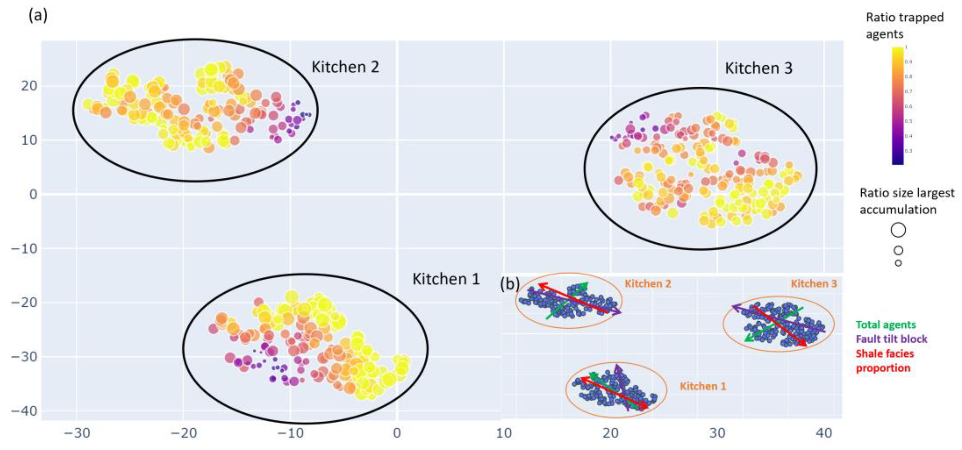
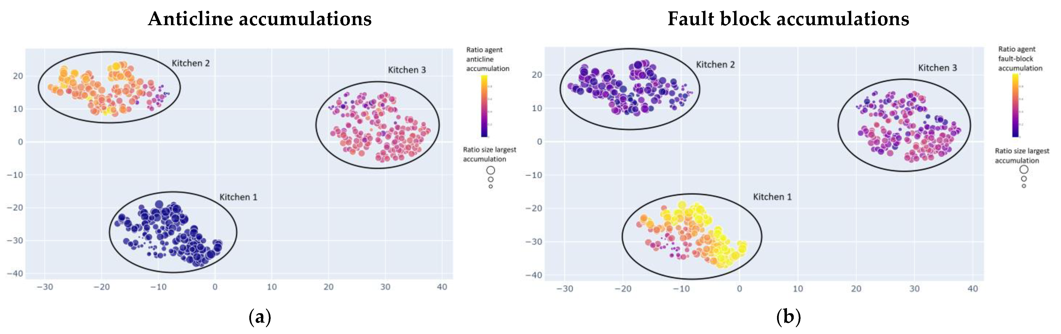
3.2.2. Sensitivity Analyses—Identification of Main Migration Drivers and Geological Uncertainties; Evaluation of the Monte Carlo Simulations
- (1)
- Accumulation size
- (2)
- Spearman correlation matrix
- (3)
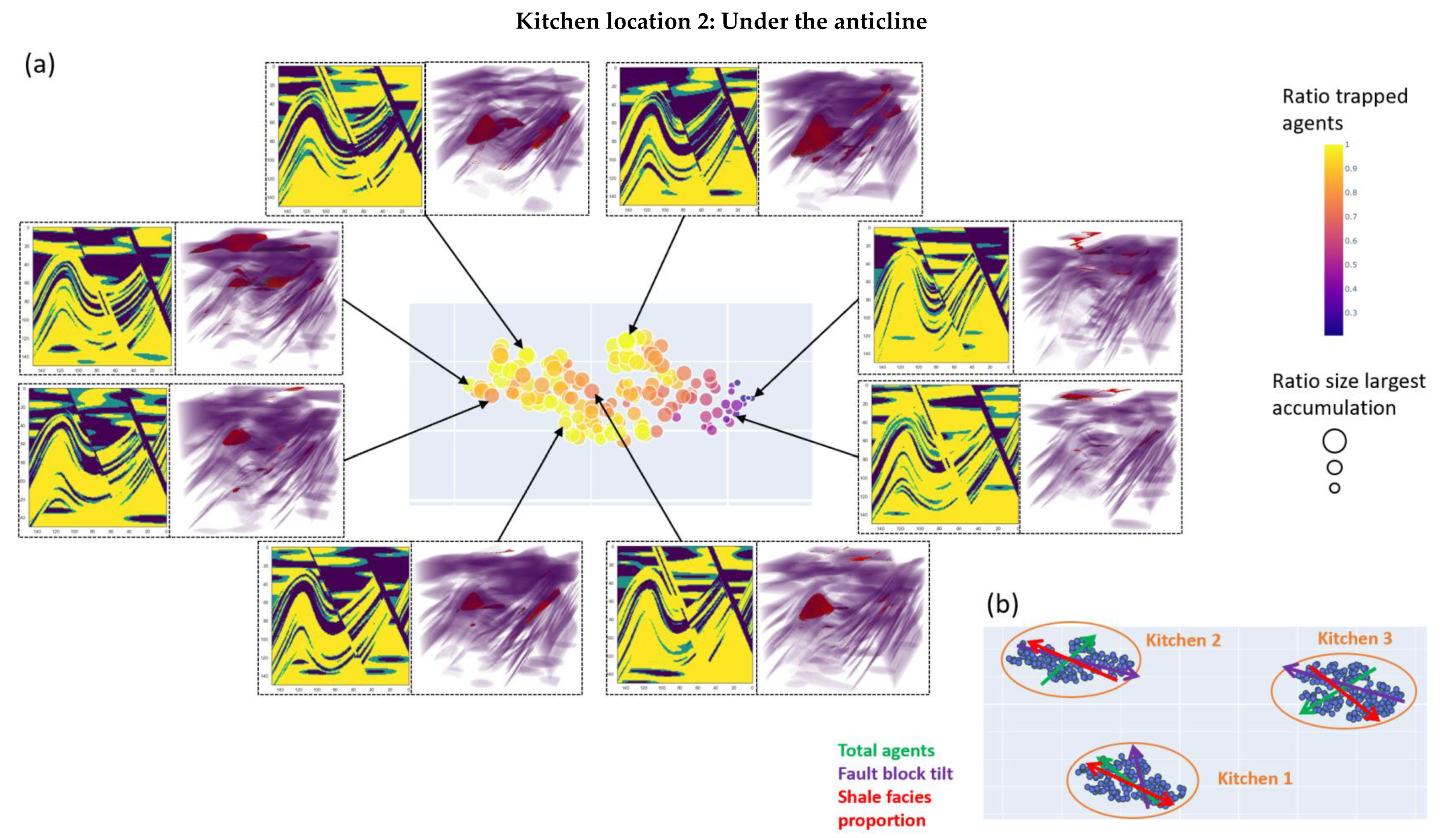
- t-SNE visualisation
- (4)
- Entropy visualisation
- (5)
- Case study evaluation
4. Discussion and Future Perspectives
5. Conclusions
Author Contributions
Funding
Institutional Review Board Statement
Informed Consent Statement
Acknowledgments
Conflicts of Interest
Appendix A

Appendix B


References
- Rodriguez, J.F.; Littke, R. Petroleum generation and accumulation in the Golfo San Jorge Basin, Argentina: A basin modeling study. Mar. Pet. Geol. 2001, 18, 995–1028. [Google Scholar] [CrossRef]
- Al-Hajeri, M.M.; Al Saeed, M.; Derks, J.; Fuchs, T.; Hantschel, T.; Kauerauf, A.; Neumaier, M.; Schenk, O.; Swientek, O.; Tessen, N.; et al. Basin and petroleum system modeling. Oilfield Rev. 2009, 21, 14–29. [Google Scholar]
- Magoon, L.B.; Dow, W.G. The petroleum system: From source to trap. AAPG Mem. 1994, 60, 93–120. [Google Scholar]
- Baur, F.; Wielens, H.; Littke, R. Basin and Petroleum Systems Modeling at the Jeanne d’Arc and Carson Basin offshore Newfoundland, Canada. Recorder 2009, 34, 28–36. [Google Scholar]
- Peters, K.E.; Curry, D.J.; Kacewicz, M. An overview of basin and petroleum system modeling: Definitions and concepts. In Basin Modeling: New Horizons in Research and Applications: AAPG Hedberg Series; American Association of Petroleum Geologists: Tulsa, OK, USA, 2012; Volume 4, pp. 1–16. [Google Scholar] [CrossRef]
- Welte, D. Petroleum systems modeling: A guidance tool for the upstream petroleum industry. Energy Explor. Exploit. 2002, 20, 401–405. [Google Scholar] [CrossRef]
- Sylta, Ø. Analysing exploration uncertainties by tight integration of seismic and hydrocarbon migration modelling. Pet. Geosci. 2008, 14, 281–289. [Google Scholar] [CrossRef]
- Tømmerås, A.; Sylta, Ø.; Daszinnies, M.C.; Mencaroni, D. Prewell and postwell predictions of oil and gas columns using an iterative Monte Carlo technique with three-dimensional petroleum systems modeling. AAPG Bull. 2018, 102, 709–728. [Google Scholar] [CrossRef]
- Tong, Y. Basin and Petroleum System Modeling with Uncertainty Quantification: A Case Study on the Piceance Basin, Colorado; Stanford University: Stanford, CA, USA, 2016. [Google Scholar]
- The Impact of DHIs on Exploration Performance, Westwood Global Energy Group. Available online: https://www.westwoodenergy.com/reports/global-ea/the-impact-of-dhis-on-exploration-performance (accessed on 24 June 2021).
- Peters, K.E.; Walters, C.C.; Mankiewicz, P.J. Evaluation of kinetic uncertainty in numerical models of petroleum generation. AAPG Bull. 2006, 90, 387–403. [Google Scholar] [CrossRef]
- Chang, H.; Liao, Q.; Zhang, D. Benchmark problems for subsurface flow uncertainty quantification. J. Hydrol. 2015, 531, 168–186. [Google Scholar] [CrossRef]
- Riva, M.; Guadagnini, A.; De Gaspari, F.; Alcolea, A. Exact sensitivity matrix and influence of the number of pilot points in the geostatistical inversion of moment equations of groundwater flow. Water Resour. Res. 2010, 46. [Google Scholar] [CrossRef]
- Rogers, D.W.O. Fifty years of Monte Carlo simulations for medical physics. Phys. Med. Biol. 2006, 51, R287. [Google Scholar] [CrossRef] [PubMed]
- Ojeda, P.; Garcia, M.; Londono, A.; Chen, N.Y. Monte Carlo Simulations of Proteins in Cages: Influence of Confinement on the Stability of Intermediate States. Biophys. J. 2009, 96, 1076–1082. [Google Scholar] [CrossRef] [PubMed]
- Tartakovsky, D.M. Assessment and management of risk in subsurface hydrology: A review and perspective. Adv. Water Resour. 2013, 51, 247–260. [Google Scholar] [CrossRef]
- Wendebourg, J.; Trabelsi, K. How wrong can it be? Understanding uncertainty in petroleum systems modelling. In Petroleum Geology Conference Series; Geological Society: London, UK, 2005; Volume 6, pp. 1289–1299. [Google Scholar]
- Kuhn, P.P.; di Primio, R.; Hill, R.; Lawrence, J.R.; Horsfield, B. Three-dimensional modeling study of the low-permeability petroleum system of the Bakken Formation. AAPG Bull. 2012, 96, 1867–1897. [Google Scholar] [CrossRef]
- Schenk, O.; Peters, K.; Burnham, A. Evaluation of alternatives to Easy% Ro for calibration of basin and petroleum system models. In Proceedings of the 79th EAGE Conference and Exhibition 2017, Paris, France, 12–15 June 2017; pp. 1–5. [Google Scholar]
- Paton, D.A.; Di Primio, R.; Kuhlmann, G.; Van Der Spuy, D.; Horsfield, B. Insights into the petroleum system evolution of the southern Orange Basin, South Africa. S. Afr. J. Geol. 2007, 110, 261–274. [Google Scholar] [CrossRef]
- Ducros, M.; Nader, F.H. Map-based uncertainty analysis for exploration using basin modeling and machine learning techniques applied to the Levant Basin petroleum systems, Eastern Mediterranean. Mar. Pet. Geol. 2020, 120, 104560. [Google Scholar] [CrossRef]
- Formaggia, L.; Guadagnini, A.; Imperiali, I.; Lever, V.; Porta, G.; Riva, M.; Scotti, A.; Tamellini, L. Global sensitivity analysis through polynomial chaos expansion of a basin-scale geochemical compaction model. Comput. Geosci. 2013, 17, 25–42. [Google Scholar] [CrossRef]
- Ruffo, P.; Porta, G.M.; Colombo, I.; Scotti, A.; Guadagnini, A. Global sensitivity analysis of geochemical compaction in a sedimentary Basin. In Proceedings of the First EAGE Basin & Petroleum Systems Modeling Workshop, Dubai, United Arab Emirates, 19–22 October 2014; Volume 1, pp. 1–5. [Google Scholar]
- Wainwright, H.M.; Finsterle, S.; Jung, Y.; Zhou, Q.; Birkholzer, J.T. Making sense of global sensitivity analyses. Comput. Geosci. 2014, 65, 84–94. [Google Scholar] [CrossRef]
- Pegaz-Fiornet, S.; Carpentier, B.; Michel, A.; Wolf, S. Comparison between the Different Approaches of Secondary and Tertiary Hydrocarbon Migration Modeling in Basin Simulators. In Basin Modeling: New Horizons in Research and Applications, AAPG Hedberg Series; American Association of Petroleum Geologists: Tulsa, OK, USA, 2012. [Google Scholar] [CrossRef]
- Hantschel, T.; Kauerauf, A.I.; Wygrala, B. Finite element analysis and ray tracing modeling of petroleum migration. Mar. Pet. Geol. 2000, 17, 815–820. [Google Scholar] [CrossRef]
- Baur, F.; di Primio, R.; Lampe, C.; Littke, R. Mass balance calculations for different models of hydrocarbon migration in the Jeanne d’Arc basin, offshore Newfoundland. J. Pet. Geol. 2011, 34, 181–198. [Google Scholar] [CrossRef]
- Baur, F.; Katz, B. Some practical guidance for petroleum migration modeling. Mar. Pet. Geol. 2018, 93, 409–421. [Google Scholar] [CrossRef]
- Darcy, H. Les Fontaines Publiques de la Ville de Dijon; Victor Dalmont: Paris, France, 1856; 647p. [Google Scholar]
- Schneider, F. Modeling multiphase flow of petroleum at the sedimentary basin scale. J. Geochem. Explor. 2003, 78, 693–696. [Google Scholar] [CrossRef]
- Wolf, S.; Faille, I.; Pegaz-Fiornet, S.; Willien, F.; Carpentier, B. A new innovating scheme to model hydrocarbon migration at basin scale: A pressure-saturation splitting. In Basin Modeling: New Horizons in Research and Applications: AAPG Hedberg Series; American Association of Petroleum Geologists: Tulsa, OK, USA, 2012; Volume 4, pp. 197–205. [Google Scholar] [CrossRef]
- Sylta, Ø. A probabilistic approach to improved geological knowledge and reduced exploration risks using hydrocarbon migration modelling. Pet. Geosci. 2004, 10, 187–198. [Google Scholar] [CrossRef]
- Carruthers, D.J. Transport Modelling of Secondary Oil Migration Using Gradient-Driven Invasion Percolation Techniques. Ph.D. Thesis, Heriot-Watt University, Edinburgh, UK, 1998. [Google Scholar]
- Carruthers, D.J. Modeling of Secondary Petroleum Migration Using Invasion Percolation Techniques. Multidimens. Basin Modeling 2003, 7, 21–37. [Google Scholar]
- de Gennes, P.G.; Brochard-Wyart, F.; Quéré, D. Capillarity: Deformable Interfaces BT—Capillarity and Wetting Phenomena: Drops, Bubbles, Pearls, Waves. In Capillarity Wetting Phenom; Springer: New York, NY, USA, 2004; Volume 336. [Google Scholar]
- Glass, R.J.; Yarrington, L. Mechanistic modeling of fingering, nonmonotonicity, fragmentation, and pulsation within gravity/buoyant destabilized two-phase/unsaturated flow. Water Resour. Res. 2003, 39. [Google Scholar] [CrossRef]
- Cavanagh, A.; Rostron, B. High-resolution simulations of migration pathways and the related potential well risk at the IEAGHG Weyburn-Midale CO2 storage project. Int. J. Greenh. Gas Control. 2013, 16, S15–S24. [Google Scholar] [CrossRef]
- Sylta, Ø. Hydrocarbon Migration Modeling and Exploration Risk. Ph.D. Thesis, Norwegian University of Science and Technology, Trondheim, Norway, 2004; 200p. [Google Scholar]
- Vasseur, G.; Luo, X.; Yan, J.; Loggia, D.; Toussaint, R.; Schmittbuhl, J. Flow regime associated with vertical secondary migration. Mar. Pet. Geol. 2013, 45, 150–158. [Google Scholar] [CrossRef]
- Cavanagh, A.; Ringrose, P. Simulation of CO2 distribution at the In Salah storage site using high-resolution field-scale models. Energy Procedia 2011, 4, 3730–3737. [Google Scholar] [CrossRef]
- Hantschel, T.; Kauerauf, A.I. Fundamentals of Basin and Petroleum Systems Modelling; Springer Science & Business Media: Berlin/Heidelberg, Germany, 2009. [Google Scholar] [CrossRef]
- Bonabeau, E. Agent-based modeling: Methods and techniques for simulating human systems. Proc. Natl. Acad. Sci. USA 2002, 99, 7280–7287. [Google Scholar] [CrossRef]
- Macal, C.M.; North, M.J. Tutorial on agent-based modelling and simulation. J. Simul. 2010, 4, 151–162. [Google Scholar] [CrossRef]
- Wilensky, U.; Rand, W. An Introduction to Agent-Based Modeling: Modeling Natural, Social, and Engineered Complex Systems with NetLogo; Massachusetts Institute of Technology, MIT Press: Cambridge, MA, USA, 2015. [Google Scholar]
- Tranouez, P.; Bertelle, C.; Olivier, D. Changing the level of description of a fluid flow in an agent-based simulation. In Proceedings of the ESS 2001, the 13th European Simulation Symposium, Marseille, France, 18–20 October 2001. [Google Scholar]
- Hunt, J.M. Petroleum Geochemistry and Geology; W.H. Freeman and Company: San Francisco, CA, USA, 1979; p. 390. [Google Scholar]
- Schowalter, T.T. Mechanics of secondary hydrocarbon migration and entrapment. AAPG Bull. 1979, 63, 723–760. [Google Scholar] [CrossRef]
- Berg, R.R. Capillary pressures in stratigraphic traps. AAPG Bull. 1975, 59, 939–956. [Google Scholar]
- Hubbert, M.K. Entrapment of petroleum under hydrodynamic conditions. AAPG Bull. 1953, 37, 1954–2026. [Google Scholar]
- Thomas, M.M.; Clouse, J.A. Scaled physical model of secondary oil migration. AAPG Bull. 1995, 79, 19–28. [Google Scholar]
- Brooks, R.H.; Corey, A.T. Properties of porous media affecting fluid flow. J. Irrig. Drain. Div. 1966, 92, 61–88. [Google Scholar] [CrossRef]
- Downey, M.W. Evaluating seals for hydrocarbon accumulations. Am. Assoc. Pet. Geol. Bull. 1984, 68, 1752–1763. [Google Scholar] [CrossRef]
- Xeek. Available online: https://xeek.ai/challenges/go-with-the-flow/overview (accessed on 22 June 2021).
- Metropolis, N.; Ulam, S. The Monte Carlo Method. J. Am. Stat. Assoc. 1949, 44, 335–341. [Google Scholar] [CrossRef]
- GemPy. Available online: https://www.gempy.org/ (accessed on 22 June 2021).
- Varga, M.D.L.; Schaaf, A.; Wellmann, F. GemPy 1.0: Open-source stochastic geological modeling and inversion. Geosci. Model Dev. 2019, 12, 1–32. [Google Scholar] [CrossRef]
- PyKrige. Available online: https://github.com/GeoStat-Framework/PyKrige (accessed on 22 June 2021).
- Murphy, B.S. PyKrige: Development of a Kriging Toolkit for Python. In Proceedings of the American Geophysical Union, Fall Meeting 2014, San Francisco, CA, USA, 15–19 December 2014. H51K-0753. [Google Scholar]
- Matheron, G. Le Krigeage Universel; École Nationale Supérieure des Mines de Paris: Paris, France, 1969; Volume 1. [Google Scholar]
- Yielding, G.; Freeman, B.; Needham, D.T. Quantitative fault seal prediction. AAPG Bull. 1997, 81, 897–917. [Google Scholar] [CrossRef]
- Harris, D.; Yielding, G.; Levine, P.; Maxwell, G.; Rose, P.T.; Nell, P. Using Shale Gouge Ratio (SGR) to model faults as transmissibility barriers in reservoirs: An example from the Strathspey Field, North Sea. Pet. Geosci. 2002, 8, 167–176. [Google Scholar] [CrossRef]
- Barton, C.A.; Zoback, M.D.; Moos, D. Fluid flow along potentially active faults in crystalline rock. Geology 1995, 23, 683–686. [Google Scholar] [CrossRef]
- Campello, R.J.; Moulavi, D.; Sander, J. Density-Based Clustering Based on Hierarchical Density Estimates; Springer: Berlin/Heidelberg, Germany, 2013; Volume 7819 LNAI, pp. 160–172. [Google Scholar] [CrossRef]
- McInnes, L.; Healy, J.; Astels, S. Hdbscan: Hierarchical density based clustering. J. Open Source Softw. 2017, 2, 205. [Google Scholar] [CrossRef]
- Spearman, C. “General Intelligence”, Objectively Determined and Measured. Am. J. Psychol. 1904, 15, 59–73. [Google Scholar] [CrossRef]
- Van Der Maaten, L.; Hinton, G. Visualizing data using t-SNE. J. Mach. Learn. Res. 2008, 9, 2579–2605. [Google Scholar]
- Balamurali, M.; Silversides, K.L.; Melkumyan, A. A comparison of t-SNE, SOM and SPADE for identifying material type domains in geological data. Comput. Geosci. 2019, 5, 78–89. [Google Scholar] [CrossRef]
- Balamurali, M.; Melkumyan, A. t-SNE based visualisation and clustering of geological domain. In Proceedings of the International Conference on Neural Information Processing, Kyoto, Japan, 16–21 October 2016; pp. 565–572. [Google Scholar] [CrossRef]
- Shannon, C.E. A Mathematical Theory of Communication. Bell Syst. Tech. J. 1948, 27, 379–423. [Google Scholar] [CrossRef]
- Wellmann, J.F.; Regenauer-Lieb, K. Uncertainties have a meaning: Information entropy as a quality measure for 3-D geological models. Tectonophysics 2012, 526, 526–529. [Google Scholar] [CrossRef]
- Griffith, D. (Shell, Cypress, Texas, USA). Personal Communication, Material was internal non published 3d seismic. 30 September 2020.
- Bjørkum, P.A.; Walderhaug, O.; Nadeau, P.H. Physical constraints on hydrocarbon leakage and trapping revisited. Pet. Geosci. 1998, 4, 237–239. [Google Scholar] [CrossRef]


| Type of Uncertainty | Location | Parameter | Range of Uncertainty |
|---|---|---|---|
| Structural | A | Fault dip | Normal distribution 45–55° |
| A | Fault offset | Normal distribution 0–200 m | |
| B | Fault block tilt | Normal distribution 0–40° | |
| Property modelling | A | Fault critically stressed | True (50%) or False (50%) |
| C | Shale facies proportion—proportion of barriers | Normal distribution 50–90% | |
| C | Shale anisotropy direction (y/x anisotropy) | Normal distribution 0.5–2 | |
| D | Silt facies proportion—proportion of pathways | Normal distribution 50–80% | |
| D | Silt anisotropy direction (y/x anisotropy) | Normal distribution 0.5–2 | |
| Source rock | E | Kitchen location | Right side of the fault (1/3), left side (1/3) or all bottom layer (1/3) |
| E | New agents per turns | Normal distribution 10–100 agents | |
| E | Number of turns | Normal distribution 200–2000 turns |
Publisher’s Note: MDPI stays neutral with regard to jurisdictional claims in published maps and institutional affiliations. |
© 2022 by the authors. Licensee MDPI, Basel, Switzerland. This article is an open access article distributed under the terms and conditions of the Creative Commons Attribution (CC BY) license (https://creativecommons.org/licenses/by/4.0/).
Share and Cite
Steffens, B.; Corlay, Q.; Suurmeyer, N.; Noglows, J.; Arnold, D.; Demyanov, V. Can Agents Model Hydrocarbon Migration for Petroleum System Analysis? A Fast Screening Tool to De-Risk Hydrocarbon Prospects. Energies 2022, 15, 902. https://doi.org/10.3390/en15030902
Steffens B, Corlay Q, Suurmeyer N, Noglows J, Arnold D, Demyanov V. Can Agents Model Hydrocarbon Migration for Petroleum System Analysis? A Fast Screening Tool to De-Risk Hydrocarbon Prospects. Energies. 2022; 15(3):902. https://doi.org/10.3390/en15030902
Chicago/Turabian StyleSteffens, Bastian, Quentin Corlay, Nathan Suurmeyer, Jessica Noglows, Dan Arnold, and Vasily Demyanov. 2022. "Can Agents Model Hydrocarbon Migration for Petroleum System Analysis? A Fast Screening Tool to De-Risk Hydrocarbon Prospects" Energies 15, no. 3: 902. https://doi.org/10.3390/en15030902
APA StyleSteffens, B., Corlay, Q., Suurmeyer, N., Noglows, J., Arnold, D., & Demyanov, V. (2022). Can Agents Model Hydrocarbon Migration for Petroleum System Analysis? A Fast Screening Tool to De-Risk Hydrocarbon Prospects. Energies, 15(3), 902. https://doi.org/10.3390/en15030902