Abstract
Air-to-water heat pumps (HPs) are widely installed in new buildings; however, they face performance degradation with high temperature emission systems, which is typical of existing buildings, or during domestic hot water (DHW) production. Hybrid systems (HSs), composed by air-to-water HPs and gas-fired boilers, can mitigate these issues by increasing the overall system efficiency. HS performance is strictly dependent on the configuration and control management of the system itself. Moreover, the building and heating plant also have a strong influence. This study presents an overview of the application of HSs that considers both space heating (SH) and DHW production, by comparing the primary energy (PE) consumption obtained by dynamic simulations. Different climates, building typologies, and DHW withdrawal profiles are used to extend the results’ validity. Additionally, several HS control strategies were implemented and compared. The results show a PE savings ranging from 5% to 22% depending on the control strategy and the external parameters applied in the simulation. The comparison of the control strategies shows that the most efficient strategies are the ones maximizing heat pump utilization. The dependence of PE savings of HS on COP values is highlighted, and a correlation is presented to provide designers with guidance on the applicability of HSs.
1. Introduction
In 2018, households represented 26% of the total final energy consumption in Europe [1]. Space heating (SH) and domestic hot water (DHW) production together represented almost 80% of the energy consumption in households [2]. Therefore, in order to meet carbon neutrality by 2050, an important contribution will necessarily come from the building sector.
Seventy-five percent of buildings were built before any standard for energy efficiency existed. These will represent the majority of the building stock in 2050. Actions need to be taken for increasing their efficiency, e.g., by adding or increasing insulation, switching to renewable heating systems, or applying smart management systems [3].
Heat pumps (HPs) are currently the most promising heating technology to be applied to decarbonize the building sector, since they can leverage the renewable share in electricity. However, heat pumps in some applications may raise some issues. DHW production as well as SH, in less insulated buildings, require high condensing temperatures that reduce the heat pumps performance, especially in colder seasons. This applies especially for air-to-water heat pumps that are, nowadays, the most sold and widespread type [4]. Thus, the intervention of a backup generator for these critical cases is often beneficial and can replace or complement the heat pump when its operation is inefficient. Moreover, the heat pump size can be reduced as it must not be sized for the peak load, avoiding oversizing and improving the part-load operation. The correct sizing of the HP generator is an important factor for enhancing the system performance [5], as well as for reducing the number of on–off cycles and for increasing the compressor’s life. Legionella prevention is another critical issue in employing heat pumps for DHW production, since the maximum water supply temperature is often not sufficient for that scope.
CO2 heat pumps can be an interesting and promising solution to be applied in high temperature applications. However, as stated by Rony et al. in [6], there are still some technical issues to be solved for the large-scale deployment of the technology.
Nowadays, air-to-water heat pumps equipped with electrical resistance are often proposed. Its operation allows for higher temperature levels but reduces the overall efficiency of the system. Alternatively, a combination of air-to-water heat pumps and gas-fired boilers is used. The number of hybrid units sold in Europe has rapidly increased from 2015 to 2018, starting from almost four thousand units sold in 2015 and reaching almost ten thousand in 2018. Now they represent approximately a 4% share of the total air-to-water heat pumps installed [4].
A number of papers showed the advantages that hybrid systems (HSs) could bring if the technology was to be developed on a large scale and with a broader strategic outlook. Zhang et al. compared different scenarios of development of the heating sector. The hybrid solution, combining heat pumps and boilers, proved to be the most versatile when compared to the adoption of full electric appliances. It could decrease the peak of electricity demand and lower the requirements for distribution heating networks [7]. In [8], three different development scenarios were compared. The scenario combining different technologies, including hybrid heat pumps, represents a compromise solution that can achieve important results in terms of emissions, decreasing the costs for users and energy systems. The economic advantages that can be derived from the adoption of hybrid systems were highlighted also by Heinen et al. [9] and in [10]. Vuillecard et al. [11] analyzed the impact on the electric grid of small-scale HSs and Näslund proposed HS application in future smart grids [12]. These studies involve more general considerations on energy strategy and infrastructure. The main findings can be summarized as follows:
- the hybrid solution could decrease the peak of electricity demand, improving the grid flexibility if complemented by smart controls;
- although it involves natural gas combustion, it is the most convenient solution from a decarbonization perspective (by fostering the HP installation in existing buildings and decreasing the costs for users and energy systems).
Combined hybrid systems for SH and DHW are widely adopted, both in single and multi-family buildings. The HS can be configured in different ways, with the generators connected in series or in parallel. The advantage of both the configurations is that the heat pump can be sized to cover only a fraction of the heat load, and the peak is covered entirely by the boiler or by the operation of both generators, depending on the control logic.
HSs have an integrated control logic, which plays a key role in system efficiency. There are many possibilities to implement it. The generators can operate in an alternate or a simultaneous way. The operation area can be divided into three zones with respect to an increasing ambient temperature: an exclusive boiler operation, a zone with simultaneous operation, and a zone where only the heat pump is switched on [13]. As described by Dongellini et al. [14] and by Bagarella et al. [15], a cut-off temperature and a bivalent temperature can be defined, respectively, as the ambient temperature at which the heat pump operation starts and as the ambient temperature at which the heat pump entirely covers the heating load. Between the cut-off temperature and the bivalent temperature, both generators can operate. The bivalent temperature defines the heat pump size if the system is designed for covering only SH loads. Otherwise, HP sizing must consider also the DHW load. The easiest control strategy is based on the coincident cut-off and bivalent temperatures. In this way, the system always works in an alternate operation. The control logic can be optimized to pursue different objectives, such as minimizing the primary energy (PE), the costs, or the CO2 emissions.
Some studies in the literature assessed the performance of a hybrid system applied to a residential building. Park et al. [16] performed an economic feasibility analysis of a hybrid system compared with a traditional gas-fired boiler applied to a 100 m2 apartment, finding that the annual cost savings can vary from 4% to approximately 9%, depending on the electricity price. Klein et al. [17] analyzed the performance of a hybrid system in series that was serving a 130 m2 apartment and found relevant primary energy savings compared to boilers. They also evaluated the influence of the size of the HP and water tanks, finding that the best performances of the hybrid system were obtained when the HP does not cover the entire building load. A weak influence of the buffer tank size on the system efficiency was found. Gang Li et al. [18] evaluated the cost reduction of different configurations of hybrid systems for DHW (20% to 65%) and SH (6% to 70%) compared with boilers. Di Perna et al. [19] assessed the performance of a hybrid system composed by a boiler and several heat pump sizes, serving the SH demand of a single-family house of 120 m2. The authors concluded that the hybrid system showed a higher efficiency than a heat pump with electric backup and compared with a boiler-only solution. Bagarella et al. [15] performed dynamic simulations of a hybrid system serving the SH load of a single-family house. They studied the influence of the cut-off temperature on the hybrid system’s efficiency. According to their results, a cut-off temperature lower than the bivalent temperature is convenient when a smaller heat pump size is selected. The economic evaluation showed advantages of the hybrid system due to the lower electricity, as well as gas consumption and lower investment costs. Dongellini et al. [14] evaluated the PE savings for hybrid systems in comparison to the monovalent system through dynamic simulations of a hybrid system with different HP sizes. They achieved higher benefits applying a parallel operation strategy, in which the boiler and heat pump operate at the same time, instead of an alternate operation. Savings obtained with respect to the monovalent HP case were of 2–3%, while the PE savings obtained in comparison with the boiler-only solution were more relevant. In a subsequent study, Dongellini et al. [20] analyzed the efficiency and the PE consumption of a hybrid system connected in series. The system provides the SH demand of a 140 m3 residential building located in the Italian city of Bolzano. The hybrid system with different heat pump sizes was simulated with TRNSYS, and the results were compared with that of a monovalent system (HP and boiler). The results lead to the conclusion that hybrid systems can achieve considerable PE savings compared to the heat pump or the boiler-only system (6% and 22%, respectively). They also concluded that the heat pump size and control strategy play an important role in HS performance.
These studies evidence that the application of HSs can obtain energy and cost savings compared to heat pump-only and boiler-only solutions. However, most of the studies that performed a simulation aimed at evaluating the system performance throughout the heating season did not consider the combined production of SH and DHW. Most of them did not compare different hybrid configurations or did not simulate different building features, as well as not having considered different climates. In general, these results support the application of HSs, however, they are valid only for the test cases examined. A comprehensive view, marking the differences in performance when the type of building, the climate, or the system configuration vary, is still lacking. Although the number of HS installations is increasing, clear guidelines for designers and manufacturers providing the correct application of the technology are still missing. The purpose of this paper is to show the influence of varying heating loads and control logic on HS performance. This can serve in raising awareness in designers on the proper application and regulation of HSs.
From an environmental point of view, the choice for the installation of a new heating system should focus on the minimization of PE demand. In this sense, the work investigates the performance in terms of PE consumption of HSs that combine air-to-water HPs and gas-fired boilers for different climatic conditions, building insulation, and DHW withdrawal profiles, through dynamic simulations. Four control strategies are compared. The first two involve a parallel configuration in which the generators operate in an alternating mode. The control logic is based on the definition of a fixed threshold temperature, which determines the switch between HP and boiler. One strategy is simpler and involves setting only the threshold temperature for SH, while DHW is supplied entirely by the boiler, whereas the second strategy switches between HP and boiler operation for both SH and DHW production. The third and fourth strategies allow the generators to work simultaneously and the decision of which generator to run is based on the HP COP value. A configuration in series and a parallel configuration were analyzed. The proposal and comparison of the control strategies with different switch logics between generators, different hydraulic configurations, and different levels of complexity represents an element of the novelty of the study. The comparison is not performed using punctual operating conditions, but rather each configuration is tested under different climatic conditions, different building thermal loads, and different load ratios between DHW and SH, which were simulated for an entire calendar year.
2. Materials and Methods
The scope of the work is to compare the performance of different HS configurations in terms of PE consumption. Firstly, a model of the HS was developed in the MATLAB R2020b environment, simulating the operation of the generators and the combined control logic. Secondly, the HS model was combined with a dynamic building simulation code, namely TRNSYS 2018, in a co-simulation framework. The simulation described in [21] was adapted and the generator was replaced with the new MATLAB model capable of emulating HS operation. TRNSYS performs the transient energy balance of the building and the primary and secondary hydronic loops. The heat produced by the hybrid system is stored in the SH and in the DHW tanks. These tanks are then connected to the tapping points and to the radiators, or the radiant panels, through the secondary loop (Figure 1). Five minutes is the timestep used in the TRNSYS simulation, which is consistent with the model characteristics and accurate enough for the analysis target.
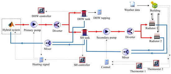
Figure 1.
Schematic of the TRNSYS simulation.
2.1. Simulation Parameters
External parameters have a strong influence on the efficiency of the hybrid system. In this paper, climate, building insulation, heating emission system, and the DHW withdrawal profile varies throughout the simulation runs.
The climates applied in the building energy simulations shall be representative of different climatic zones in Europe. Two reference cities were identified starting from the climatic zone classification for building energy simulations proposed by Gasparella & Pernigotto [22]. According to the classification, Europe is divided into four main climatic areas. In the present work, we focused on the cold climate typical of eastern Europe and part of the alpine region, and on the temperate climate typical of western Europe. The two representative cities are respectively Prague, with 3703 heating degree-days (HDD18), and Strasbourg (HDD18 = 2947). Climatic data were retrieved from the Energy Plus dataset [23].
The reference buildings are selected starting from a characterization, which classifies a series of sample buildings representing the Italian building stock [24] and is based on the latest census on Italian dwellings. The characteristics of the external walls for building B1 and B2 are reported in Table 1. As the TABULA project proved [25], the Italian construction characteristics are similar to those of most of the other European countries. Two representative residential buildings, made of two heating zones of 90 m2 each with different insulation levels, are simulated. The investigated structures exhibit similar characteristics to buildings representative of single-family houses in France (i.e., SFH5 and SFH7) and the Czech Republic (SFH5 and SFH6) [25].

Table 1.
Characteristics of external wall composition of building B1 and B2.
The annual heating needs for the buildings (building consumption), the less insulated one, named B1, and the one with a higher level of thermal insulation, named B2, in the climates of Prague and Strasbourg, are summarized in Table 2.
Table 2.
Overview of simulation parameters.
Building B1 is provided with low temperature radiators. The setpoint temperature of the SH tank is adjusted by an outdoor reset control (OTR) based on the radiator efficiency curve, with a design water temperature of 52 °C and a minimum setpoint of 42 °C at an outdoor temperature of 10 °C. The water supply temperature of the generators is kept 3 °C higher than the SH setpoint temperature.
Building B2 is equipped with radiant panels. Similarly, the set point of the SH tank is set at a design temperature of 40 °C and is reduced depending on the outdoor temperature using OTR—down to a minimum of 32 °C at an outdoor temperature of 20 °C. As in building B1, the water supply temperature of the generators is kept 3 °C higher than the SH set point temperature.
Two different DHW withdrawal profiles were applied for building B2 to better assess the impact of DHW production on the overall efficiency, and to understand the effect of different values of the ratio between heating load and DHW load. One case simulates a daily water consumption of 0.25 m3, while the second one simulates a consumption of 0.55 m3 per day. These values are based on the standard profiles reported in the European norm EN 16147 [26].
The DHW tank is maintained at a fixed temperature of 55 °C and, as for the SH tank, the generators’ water supply temperature is maintained at 3 °C higher than the tank setpoint.
The size of the HP was adapted for each control strategy to fulfill the SH and DHW setpoints. The size of the boiler is kept fixed, due to its large modulation range. The sizes of the DHW and SH tanks were kept fixed through the simulations, except for cases 5 and 6, in which the increased DHW demand required higher tank volumes. DHW and SH tanks are 0.3 m3 and 0.2 m3, respectively, with a DHW daily consumption of 0.25 m3. The tanks sizes increase to 0.6 m3 and 0.3 m3 with a daily DHW consumption of 0.55 m3.
The HP and the water tank sizes were chosen simultaneously, as they are interdependent. They should be sized to cover the building heating load in case of maximum DHW withdrawal according to the considered daily profile. Given the DHW production priority, an increase in DHW withdrawal leads to less availability of generators to charge the SH storage, resulting in a reduction in its temperature. Therefore, an increase in the volume of the DHW tank also results in an increase in the size of the SH tank.
Table 2 shows an overview of the cases and parameters applied in the simulations.
2.2. Model Development
The HS model is composed of two subroutines that simulate a heat pump and a gas-fired boiler, respectively. In addition, the code is able to manage the operation and the control of the two generators by distributing the load between them, according to the configuration considered.
Several modeling strategies can be pursued; nonetheless, the model should be appropriate for the scope of the study. In fact, a more complex model does not automatically provide more accurate results, since a higher complexity can lead to incremented errors [27,28]. The model has to simulate accurately the transient operation phases, in case of enhanced HVAC design. However, the longer time response of the building allows for the assumption of perfect control and idealized operation for the building energy simulation [29]. Following these considerations, the HS model was developed on the basis of performance maps. The heat pump and the boiler models are based on performance data provided by manufacturers to replicate the performance of commercially available systems.
The heat pump model refers to modulating heat pumps, which are provided with an R410a refrigerant, inverter driven compressor, EC axial fans, and electronic expansion valve (EEV). The capacity varies from 8 to 30 kW, defined at 7 °C ambient temperature and 35 °C water supply temperature, with respect to the application. The heat pump COP at full load is equal to 3.6, at the specified ambient conditions. The minimum step of modulation achieves a capacity of 40% compared to the nominal one. The boiler model refers to a condensing boiler of 35 kWp and a modulation that is down to 10% of the peak capacity, with an efficiency, referred to as the lower heating value, at 80 °C/60 °C supply and return water temperatures of 97.7%.
The model of the HP is based on multivariable interpolation of performance data. The model determines the heating capacity and power input based on the source and sink temperatures and capacity modulation. Similarly, the boiler model calculates the heating capacity and fuel mass flow rate, starting from the inlet and outlet water temperatures and modulation rate.
Figure 2 shows a simplified scheme of the logic of the HS model and its combination with the TRNSYS simulation. The HS model receives, as an input, the outdoor boundary conditions (Tair, RH), the mass flow rate (mw), the return water temperature from the water tanks (Twin), and the control signal (i.e., turn-on in case of heating demand from SH or DHW). Based on this, initially the control logic calculates the set point and chooses whether to activate the heat pump, the boiler, or both generators (further details about HS control strategies are provided in Section 2.3). After that, the modulation control section identifies the most suitable modulation for the generator that is operating, based on the required set point. Each generator works between a maximum and a minimum modulation. A dead band is implemented in order to keep the outlet water temperature within the predefined threshold values. The HP and boiler models are executed, and the resulting water supply temperature is passed to the TRNSYS simulation. Other performance figures calculated from the HS model are stored and used for the subsequent analysis.
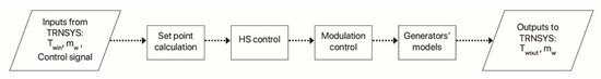
Figure 2.
Schematic of HS model.
According to Clauß and Laurent [30], heat pump models developed to be connected to building simulations often suffer from excessive simplifications and this may affect the final results. The goal of this study was to reproduce the behavior of the system as close to reality as possible by seeking a trade-off between accuracy and computational cost. The most relevant considerations made during the development of the hybrid system (boiler and heat pump) model are reported below:
- The model is based on the performance data at full load and part load operation. When the minimum load is reached, the heat pump is switched off. It is recognized that heat pump cycling losses play an important role in heat pump seasonal performance. In this work, a penalty factor was introduced to take this phenomenon into account, according to the results obtained by Bagarella et al. [31], who performed experimental evaluations for the determination of cycling losses;
- The model of the boiler is also based on the performance data at full and part load operation. The startup phase was modelled according to the information provided by the manufacturer. The boiler follows an ignition ramp during startup, before setting at the desired modulation;
- The need for defrosting at certain outdoor conditions is a critical point in heat pump systems. In this work, the approach proposed by Zhu et al. [32] that identifies four different defrosting risk-zones was adopted. The performance degradation was simulated based on the results obtained by Chen and Guo [33] on a similar type of heat pump;
- The heat pump source and sink temperature limits are implemented into the model;
- A minimum downtime after the heat pump is turned off is established to increase the durability of the compressor. The minimum downtime set for the boiler is based on the settings reported by the boiler manufacturer;
- The water tank model includes the simulation of the stratification process in order to obtain return water temperatures as close as possible to the real ones;
- DHW production is prioritized, as it is set in most field applications. As is described in Section 2.1, this influences the choice of the water tank and heat pump size.
2.3. Control Strategies
Several control strategies were implemented to identify the most effective ones in terms of PE savings, and to estimate if an increase in the control strategy complexity would lead to an appreciable increase in savings.
The primary energy is calculated, at each timestep, according to the following equation:
where fpen and fpng represent the primary energy conversion factors (PECFs) of electricity and natural gas. The values considered for the PECFs are the reference EU values, derived from the informative table B.16 of the European standard EN ISO 52000-1 [34].
The value of PE used in the analysis is the sum of the values for each timestep throughout the simulation run.
The implemented control strategies are listed here below:
HP: it is the reference case. The building load (SH + DHW) is provided by a heat pump that is sized for covering the total heat load.
CS1: it refers to the hybrid system described by the flow diagram in Figure 3. Under this control strategy, the boiler provides the entire DHW demand. The SH demand is provided by the heat pump when the outdoor temperature is above a certain threshold (Tth-SH). The boiler operates at ambient temperatures lower than Tth-SH.
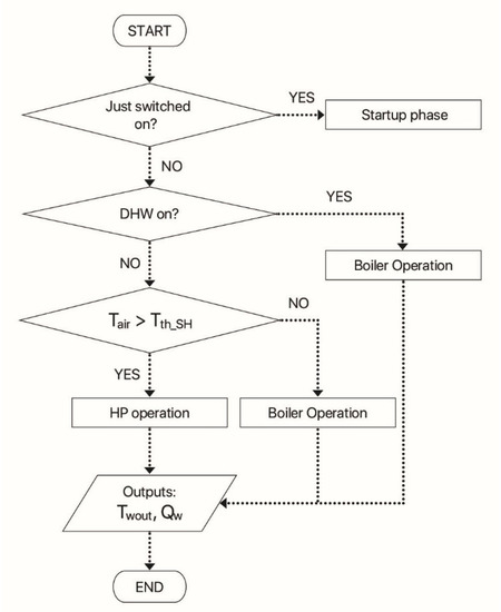
Figure 3.
Flowchart relative to CS1.
CS2: in this case, a threshold temperature for SH (Tth-SH) and one for DHW (Tth-DHW) are determined. The boiler operates when the ambient temperature is below Tth-SH for SH demand, and when the temperature is below Tth-DHW, in case of DHW demand. The heat pump operates when the ambient temperature is above Tth-SH for SH demand, and when the temperature is above Tth-DHW, in case of DHW demand (Figure 4).
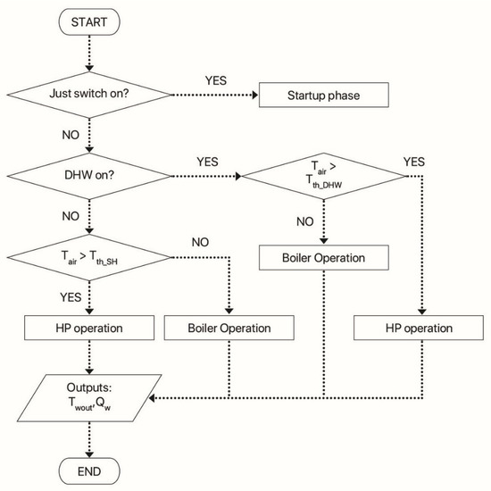
Figure 4.
Flowchart relative to CS2.
CS3: configuration “in series”. The return water from the tanks flows first through the heat pump and then through the boiler. Figure 5 shows the hydraulic layout of the strategy, and the control logic is explained in the diagram in Figure 6. A threshold value of the COP (COPlim) is introduced to determine if the heat pump operation is more convenient than the boiler one in terms of PE consumption. A more in-depth explanation would be that COPlim represents the COP value of the HP at which the PE consumed by the HP equals the PE consumed by the boiler for the same amount of energy supplied in a given timestep. If the estimated COP is greater or equal to COPlim, the heat pump will run for that timestep, while the boiler remains switched off. If not, the control logic lowers the heat pump setpoint temperature and checks if the COP increases above COPlim. If so, both the heat pump and the boiler operate, and the boiler receives incoming water flow from the heat pump. If COPlim is not reached, only the boiler operates. COPlim is calculated according to the formula:
ηboiler_mean represents the average value of the boiler efficiency and is suitable to be used when the boiler operates within the operating temperatures used in the case study. As the PECF values are taken from the reference EU standard, the value of COPlim is the same for all the cases considered. In the model, HP operation is simulated, and the COP is compared with COPlim. In real systems, the strategy can be applied by implementing the HP COP curve in the control logic, which can then estimate the COP at the required operating conditions based on the ambient temperature and the required set point and compare it with COPlim. Therefore, this strategy requires a more sophisticated control logic compared with CS1 and CS2.
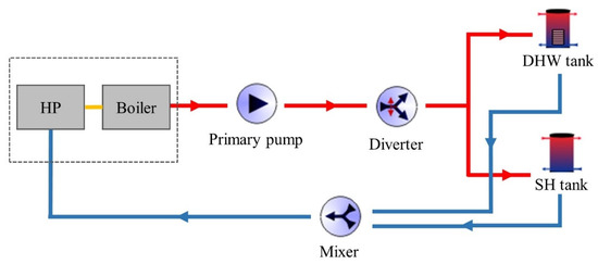
Figure 5.
CS3 configuration—hydraulic layout of the primary hydronic loop.
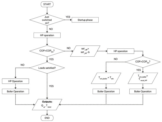
Figure 6.
Flowchart relative to CS3.
The boiler also works as an integration to the heat pump when the capacity of the heat pump is not sufficient to cover the loads. The control over the HP’s ability to meet the demand is done by monitoring the return water temperature. If the return water temperature is colder than the previous timestep, then the energy drawn from the tank is greater than that supplied by the HP, and thus the heating load could not be satisfied. A time-based method could also be applied in real systems. A parameter representing a time constant is implemented and the system decides that the load is not satisfied when the set point is not reached within the time specified by the parameter.
CS4: configuration “in parallel”. The heat pump and boiler operate on separate primary circuits. The heat pump or boiler operation is determined based on COPlim, as in CS3. The supply and return of the heat pump and boiler are connected to the water inlets and outlets of the tanks at different heights. In this way, being the heat pump connected at a lower height in the stratified water tank, it can work at lower temperature levels, enhancing its efficiency. The boiler works when its operation is more efficient or when a capacity integration is necessary. Figure 7 shows the hydraulic layout of the strategy, whose implementation required an adaptation of the primary loop of the TRNSYS simulation layout, and the control logic relative to CS4 is explained in the diagram in Figure 8. The same considerations on the control logic made for CS3 apply also for CS4.
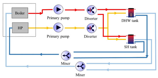
Figure 7.
CS4 configuration—hydraulic layout of the primary hydronic loop.
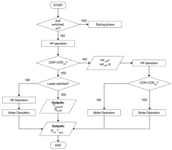
Figure 8.
Flowchart relative to CS4.
The efficacy of strategies CS1 and CS2 is strictly linked to the choice of the threshold temperatures of switch between the heat pump and boiler for SH and DHW. For this reason, the threshold temperature that minimizes the primary energy consumption was determined through a sensitivity analysis. A series of simulations was performed varying the switch temperature between the boiler and heat pump and seeking for the temperature that minimizes the PE consumption. Four optimal threshold temperatures for SH (Tth-SH) were determined, since cases 5 and 6 adopt the same SH settings as cases 3 and 4. Additionally, four DHW threshold temperatures (Tth-DHW) were determined in the same way for cases 1, 3, 5, and 6.
A series of simulations with the monovalent heat pump system and the four hybrid system control strategies were performed for each case shown in Table 2. The goal was to identify the most efficient solution in terms of PE consumption.
3. Results
The previous section described how the simulation framework is structured. More in detail, the control strategies implemented, and the parameters considered for each of the six cases listed in Table 2 were described. With this premise, firstly, the sensitivity analysis for the determination of Tth-SH and Tth-DHW to be applied to the control strategies CS1 and CS2 was performed. Different threshold values for SH and DHW were determined, as the system set point for DHW differs from the one used for SH. The methodology used for the determination of the threshold temperature can be found in Figure 9 and Figure 10. They show the total PE consumption of the one-year simulation obtained with CS1 at different threshold temperatures (Tth-SH). Four optimal values of threshold temperature for space heating (Tth-SH) were determined, as cases 5 and 6 replicate the space heating settings of case 3 and 4. The optimal Tth-SH for cases 1 and 2 is equal to 5.5 °C and the optimal Tth-SH for cases 3 and 4, and cases 5 and 6, is equal to 2 °C. The same procedure was adopted to determine the optimal DHW threshold temperature values (Tth-DHW).
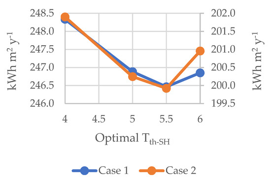
Figure 9.
Determination of optimal Tth-SH for case 1 and 2.
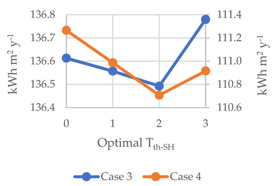
Figure 10.
Determination of optimal Tth-SH for case 3 and 4.
The summary of the resulting Tth-SH and Tth-DHW for all cases can be found in Table 3. These threshold values were used for the implementation of CS1 and CS2.
Table 3.
Optimal values of threshold temperature for SH and DHW (Tth-SH and Tth-DHW) for case 1–case 6.
In Figure 11, the optimal Tth-SH obtained were related to the average water supply temperature calculated during the heating season, showing a correlation between them.
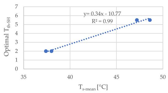
Figure 11.
Optimal values of Tth-SH as a function of the average water supply temperature of the generators (Ts-mean) in case 1 to case 4.
Then, the simulations with the heat pump system and the four hybrid system control strategies were performed for each case. The results are summarized in Table 4. The table shows the size of the HP selected for the simulation (Pref) at standard working conditions (35 °C water supply temperature and 7 °C ambient temperature), the PE savings compared to the HP (reference case), and the ratio between the total energy provided by the HP and the total energy provided by the system (boiler + HP) to the water in the simulation (ER). The value of ER represents the load distribution between the boiler and heat pump for each control logic adopted and for each case. Case 1 shows the highest building annual energy demand (191 kWh m−2 y−1), as well as the highest PE savings of the hybrid system compared to the heat pump solution. PE savings almost reach 22% with all hybrid system control strategies, except for the configuration in parallel (CS4). The highest ER provided by the heat pump is reached by the configuration in series. Similar results can be observed for case 2. Savings of approximately 17% can be reached by the hybrid control strategies CS1 to CS3, while the configuration in parallel reaches approximately 12%. The highest ER from HP is achieved again by CS3. Case 3 and 4 show a similar tendency in the results. However, smaller PE savings are obtained. The most convenient strategies in terms of PE savings are CS2 and CS3, with an advantage for CS3 of approximately 1% for both cases 3 and 4. CS3 also leads to the highest ER. The effect of increased DHW demand in cases 5 and 6 causes CS1 to save significantly less PE than the other hybrid configurations. This is due to the fact that the HP is not used for DHW production and it is particularly visible for case 6, where the ratio between DHW demand and total energy demand is the highest (31%). The best performance in terms of PE savings is achieved by CS3 in cases 5 and 6, reaching 13.6% and 10.1%, respectively.
Table 4.
Heat pump size (Pref), PE savings, and ER in the HP and CS1—CS4 configuration for case 1–case 6.
A subsequent analysis of cases 1 through 4, having the same DHW load, shows the dependence of PE savings as a function of some selected variables. PE savings are analyzed as a function of building consumption, average source and sink temperatures, and COP value of the heat pump calculated at these temperatures.
Figure 12 shows a linear correlation between building consumption and the savings obtained with the best strategy for the hybrid system applied to cases 1 through 4. The configuration in series was chosen as the best strategy as it provides the best—or comparable—HS savings among the other control strategies for all cases.
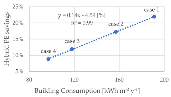
Figure 12.
Correlation between the maximum savings obtained with the hybrid configuration and the building consumption.
Figure 13 shows the correlation between the PE savings of CS3 for each case, and the difference between the water supply temperature for SH (Ts-mean) and the mean ambient temperature during the heating season (Tair-mean). A linear correlation can be detected between PE savings and the difference between Ts-mean and Tair-mean.
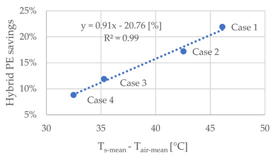
Figure 13.
Correlation between the maximum savings obtained with the hybrid configuration and the difference Ts-mean − Tair-mean.
A linear correlation is observed also in Figure 14, showing the COP values calculated at Ts-mean and Tair-mean for cases 1 through 4.
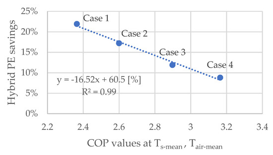
Figure 14.
Heat pump COP values calculated at Tair-mean and Ts-mean for case 1 to case 4.
4. Discussion
The analysis performed for the determination of the optimal threshold temperature for the control strategies CS1 and CS2 shows that the optimal values of Tth-SH vary according to the building used in the simulation (5.5 °C for B1, 2 °C for B2). Different types of emitters are applied, radiators in B1 and radiant panels in B2, and, therefore, the generators operate with different setpoint temperatures. It can be inferred that the optimal threshold temperature values depend on the water supply temperature levels, as in Figure 11. The COP of the heat pump is highly dependent on the water supply temperature. This also affects the efficiency of the HP relative to that of the boiler. The water supply temperature required for the generator is directly proportional to the threshold value of the ambient temperature at which the boiler is stopped, and the HP starts operating.
The results reveal that the climate in which the building is located, and consequently the ambient temperature, does not influence the optimal value of the threshold temperature. The reason is that the optimal Tth-SH identifies a threshold above which the heat pump is more efficient than the boiler, and vice versa below. The optimal value of Tth-SH does not depend on how much time the ambient temperature is below or above this threshold.
The same considerations can be made regarding the optimal values of Tth-DHW. The same DHW setpoint is used for cases 1 through 6, leading to the same optimal values of Tth-DHW for all cases and confirming the observations made for Tth-SH.
With regards to the PE savings reported in Table 4, Figure 12 reveals a correlation between PE savings and building consumption. In other words, the colder the climate, the less insulated the building, and the higher the benefits of the application of a hybrid system compared with an HP-only solution.
The building with higher heating needs also requires higher water supply temperatures (cases 1 and 2). Moreover, the buildings located in colder climates (lower Tair-mean) have a higher heating load. The HS savings are higher when the water supply temperature values are higher and when ambient temperatures are lower, as shown in Figure 13. In contrast, their relative efficiency becomes lower at lower Ts-mean and at higher Tair-mean.
Therefore, the hybrid system savings depend on the characteristics of the COP curve as it is a function of the ambient temperature and, even more, of the water supply temperature. As evidenced, the COP values are linearly correlated to the HS savings, as shown in Figure 14, thus demonstrating that the latter reflect the HP efficiency curve. The COP values in the graph are evaluated at an average ambient air and water supply temperature; therefore, there is no need to perform an annual simulation to evaluate the COP used in the graph. The COP values at the average conditions of supply and ambient temperatures are easy to determine in the dimensioning phase and can be a useful guide for designers to easily assess if the application of an HS can be convenient in terms of PE savings.
The correlations reported in the figures above are valid for the range of values investigated. Considering the technical properties of the system, increasing the building load above this range would lead to a limit beyond which the HS savings will no longer increase. This is due to the limits of the heat pump water supply temperature being reached.
The comparison between the results of cases 3 and 4 with the results of cases 5 and 6 shows that an increase in DHW demand leads to a better HS performance. For case 5, and especially for case 6, the most favorable control strategies are the ones in which the heat pump contributes to the DHW demand—i.e., CS2 and CS3—whose PE savings almost double those obtained with CS1. The application of CS1 can be of interest in cases 1 and 2. In these cases, savings are very similar for all strategies with the advantage that CS1 is easier to implement.
Throughout the simulations, CS2 and especially CS3, the configuration in series, proved to be the most efficient control strategies in terms of PE consumption. CS2 and CS3 are also the control strategies that allow for the maximum exploitation of the HP (higher ER). Therefore, a more complex control strategy that adopts an optimized control for DHW production as well provides greater benefits. This is especially true for better-insulated buildings and large DHW withdrawals, while for less-insulated buildings the difference with respect to less complex strategies (CS1) is less marked.
Regarding CS3, the advantage of placing the generators in series is that they can work at different setpoints, i.e., different temperature levels, thus enhancing the HP efficiency.
Specific considerations are needed with respect to the parallel configuration (CS4). As the layout of Figure 7 shows, the heat pump and boiler are connected with the inlets and outlets of the water tanks at different heights, which correspond to different temperatures. This allows the heat pump to work at a lower temperature level during simultaneous operation of the generators. In this way, the stratification of the tanks is reduced, and the water tanks are kept at a more constant temperature, which leads to higher energy consumption—even if the set points of the tanks are equal among the control strategies. This also represents a positive aspect. In this case, smaller water tanks can be used, making the system more compact. In this work, different configurations applied to the same water tank volumes were compared. Nevertheless, a more in-depth analysis in this sense might be interesting for future studies. A preliminary evaluation has shown that the parallel configuration with smaller SH and DHW tank volumes could lead to PE savings comparable with the control strategy CS3. The HP taken as a reference in this paper is equipped with an inverter and EEV, as are most heat pumps installed for residential use today. This type of heat pump shows reduced on–off cycling losses, compared to HPs provided with a thermostatic expansion valve [31]. The maximum COP is not reached at the maximum compressor frequency. In this context, it is possible to set an adjustment that increases the time the HP works with the modulation that provides maximum efficiency. It is thus possible to increase the efficiency of the HP throughout the heating season. This strategy is harder to apply to a monovalent HP system, as it would lead to oversizing of the HP capacity. This would cause even more frequent on–offs in the mid-seasons, with possible damage to the compressor.
Having considered the reference PECF values for the EU, as well as typical EU climates, the results of the study are representative of the European situation. Nonetheless, in countries with a higher renewable share in electricity production, the lower electrical PECF reduces the COPlim value, thus extending the HP operational range.
This scenario is expected to happen over years in all the EU countries, since the share of renewables in electricity production will presumably increase in the pursuit of decarbonization goals.
5. Conclusions
The present study focused on HSs combining air-to-water heat pumps with gas-fired boilers. The aim was to provide an overview of the benefits that hybrid systems can achieve in terms of PE savings compared to HP-only solutions for different buildings and climates.
To do so, a model of the generators and their control logic was developed in MATLAB, then combined with a model of a heating system and of a building developed in TRNSYS. Dynamic simulations were carried out using several varying parameters, such as reference climate, type of building—insulation and heating emission system—and DHW withdrawal profile. A monovalent HP system and four hybrid control strategies were implemented and compared in terms of PE consumption.
The main conclusions are as follows:
- The overall most efficient control strategies with respect to PE savings are those in which the HP contribution on the heat load is the highest (CS2 and CS3), with a more complex control strategy compared to CS1;
- In buildings with high heating loads, the benefits of introducing a more complex control strategy are reduced (as CS2 and CS3 in case 1). With lower building needs (case 4) the advantage of a more complex control strategy increases;
- For higher DHW demand, a more complex control strategy should be implemented. Here, the HP contributes to DHW production;
- The dependency of the COP curve on ambient temperature and water supply temperature influences the HS PE savings. Higher PE savings are detected in high heating-load buildings. Here, the required water supply temperature is higher and the mean ambient temperature is lower;
- A correlation, based on the evaluation of the heat pump COP at fixed points, is proposed so that engineers and designers can easily obtain an initial indication on the convenience of HSs in terms of PE savings.
The study highlights the variation in performance of hybrid systems with respect to the conditions under which they are applied, and the importance of choosing the most appropriate control strategy for each case.
Energy use for heating and DHW in the existing building stock, which consists mainly of uninsulated or poorly insulated buildings, represents the main cause of energy consumption in the residential sector. This study shows that HSs can be a viable solution for increasing energy efficiency, especially of less insulated buildings, which will represent the majority of the building stock for several decades to come.
Author Contributions
Conceptualization, E.R., A.P., M.B. and P.B.; methodology, E.R., A.P. and M.B.; software, E.R. and A.P.; resources, M.B. and P.B.; writing—original draft preparation, E.R.; writing—review and editing, E.R., A.P., M.B. and P.B.; supervision, A.P. and M.B.; project administration, M.B. and P.B.; funding acquisition, M.B. and P.B. All authors have read and agreed to the published version of the manuscript.
Funding
This research was funded by the MIUR-Italian Ministry of Education, Universities and Research (PRIN 2017) grant number 2017KAAECT in the framework of FLEXHEAT project “The energy FLEXibility of enhanced HEAT pumps for the next generation of sustainable buildings”.
Conflicts of Interest
The authors declare no conflict of interest.
Abbreviations
| HP | Heat pump |
| HS | Hybrid system |
| DHW | Domestic hot water |
| SH | Space heating |
| PE | Primary energy |
| PECF | Primary energy conversion factor |
| COPlim | Threshold COP value [-] |
| Qw | Heat delivered to the water [W] |
| Qw_HP | Heat delivered to the water by the HP [W] |
| Set_HP | Heat pump set point temperature [°C] |
| Tth-SH | Threshold temperature for Space Heating [°C] |
| Tth-DHW | Threshold temperature for Domestic hot water [°C] |
| Twin | Inlet water temperature to hybrid system [°C] |
| Twin_boiler | Inlet water temperature to boiler [°C] |
| Twout | Outlet water temperature of hybrid system [°C] |
| Twout_HP | Outlet water temperature of heat pump [°C] |
| Ts-mean | Mean temperature of the generator’s water supply during the heating season [°C] |
| Tair-mean | Mean ambient temperature throughout the heating season [°C] |
| ts | Simulation timestep [s] |
| Average electric power consumption of the heat pump during one timestep [W] | |
| Average electric power consumption of the boiler during one timestep [W] | |
| Qboiler | Average fuel energy input of the boiler during one timestep [W] |
| fpen | Primary energy conversion factor for grid electricity [-] |
| fpng | Primary energy conversion factor for natural gas [-] |
| Tair | Ambient temperature [°C] |
| RH | Relative humidity [%] |
| mw | Mass flow rate of primary loop. [kg h−1] |
| Average boiler efficiency | |
| Pref | Size of the HP selected for the simulation at 35 °C water supply temperature and 7 °C ambient temperature |
| ER | Share of thermal energy supplied by the HP to the total thermal energy of the HS |
References
- Eurostat. Energy Consumption in Households—Statistics Explained. Available online: https://ec.europa.eu/eurostat/statistics-explained/index.php/Energy_consumption_in_households#Energy_consumption_in_households_by_type_of_end-use (accessed on 28 March 2021).
- Eurostat. File: Final Energy Consumption in the Residential Sector by Use, EU-27. Statistics Explained. Online Data Code: nrg_bal_c. 2018. Available online: https://ec.europa.eu/eurostat/statistics-explained/index.php?title=File:Final_energy_consumption_in_the_residential_sector_by_use,_EU-27,_2018.png (accessed on 28 March 2021).
- Publications Office of the EU. Going Climate-Neutral by 2050. Available online: https://op.europa.eu/en/publication-detail/-/publication/92f6d5bc-76bc-11e9-9f05-01aa75ed71a1 (accessed on 28 March 2021).
- EHPA Stats. Available online: http://www.stats.ehpa.org/hp_sales/story_sales (accessed on 2 June 2021).
- Bee, E.; Prada, A.; Baggio, P. Variable-Speed Air-to-Water Heat Pumps for Residential Buildings: Evaluation of the Performance in Northern Italian Climate. In Proceedings of the CLIMA 2016—12th REHVA World Congress, Alborg, Denmark, 22–25 May 2016. [Google Scholar]
- Rony, R.U.; Yang, H.; Krishnan, S.; Song, J. Recent advances in transcritical CO2 (R744) heat pump system: A review. Energies 2019, 12, 457. [Google Scholar] [CrossRef] [Green Version]
- Zhang, X.; Strbac, G.; Teng, F.; Djapic, P. Economic assessment of alternative heat decarbonisation strategies through coordinated operation with electricity system—UK case study. Appl. Energy 2018, 222, 79–91. [Google Scholar] [CrossRef]
- DELTA Energy and Environment. 2050 Pathways for Domestic Heat: Final Report. 2012. Available online: https://www.delta-ee.com/downloads/798-2050-pathways-for-domestic-heat-final-report.html (accessed on 30 April 2021).
- Heinen, S.; Burke, D.; O’Malley, M. Electricity, gas, heat integration via residential hybrid heating technologies—An investment model assessment. Energy 2016, 109, 906–919. [Google Scholar] [CrossRef]
- Imperial College London. Analysis of Alternative UK Heat Decarbonisation Pathway, Report for the Committee on Climate Change. 2018. Available online: https://www.theccc.org.uk/wp-content/uploads/2018/06/Imperial-College-2018-Analysis-of-Alternative-UK-Heat-Decarbonisation-Pathways.pdf (accessed on 10 September 2019).
- Vuillecard, C.; Hubert, C.E.; Contreau, R.; Mazzenga, A.; Stabat, P.; Adnot, J. Small scale impact of gas technologies on electric load management—μCHP and hybrid heat pump. Energy 2011, 36, 2912–2923. [Google Scholar] [CrossRef]
- Näslund, M. Hybrid Heating Systems and Smart Grid—System Design and Operation—Market Status; Project Report; Danish Gas Technology Centre: Horsholm, Denmark, 2013. [Google Scholar]
- Grassi, W. Green Energy and Technology Heat Pumps Fundamentals and Applications; Springer: Berlin/Heidelberg, Germany, 2018. [Google Scholar]
- Dongellini, M.; Morini, G.L.; Impalà, V. Design rules for the optimal sizing of a hybrid heat pump system coupled to a residential building. In Proceedings of the 16th International Conference on Sustainable Energy Technologies—SET 2017, Bologna, Italy, 17–20 July 2017. [Google Scholar]
- Bagarella, G.; Lazzarin, R.; Noro, M. Annual simulation, energy and economic analysis of hybrid heat pump systems for residential buildings. Appl. Therm. Eng. 2016, 99, 485–494. [Google Scholar] [CrossRef]
- Park, H.; Nam, K.H.; Jang, G.H.; Kim, M.S. Performance investigation of heat pump-gas fired water heater hybrid system and its economic feasibility study. Energy Build. 2014, 80, 480–489. [Google Scholar] [CrossRef]
- Klein, K.; Huchtemann, K.; Müller, D. Numerical study on hybrid heat pump systems in existing buildings. Energy Build. 2014, 69, 193–201. [Google Scholar] [CrossRef]
- Li, G.; Du, Y. Performance integration and economic benefits of new control strategies for heat pump-gas fired water heater hybrid system. Appl. Energy 2018, 232, 101–118. [Google Scholar] [CrossRef]
- Di Perna, C.; Magri, G.; Giuliani, G.; Serenelli, G. Experimental assessment and dynamic analysis of a hybrid generator composed of an air source heat pump coupled with a condensing gas boiler in a residential building. Appl. Therm. Eng. 2015, 76, 86–97. [Google Scholar] [CrossRef]
- Dongellini, M.; Naldi, C.; Morini, G.L. Influence of sizing strategy and control rules on the energy saving potential of heat pump hybrid systems in a residential building. Energy Convers. Manag. 2021, 235, 114022. [Google Scholar] [CrossRef]
- Franzoi, N.; Prada, A.; Verones, S.; Baggio, P. Enhancing PV self-consumption through energy communities in heating-dominated climates. Energies 2021, 14, 4165. [Google Scholar] [CrossRef]
- Pernigotto, G.; Gasparella, A. Classification of European Climates for Building Energy Simulation Analyses Classification of European Climates for Building Energy Simulation Analyses. In Proceedings of the International High Performance Buildings Conference, West Lafayette, IN, USA, 9–12 July 2018. [Google Scholar]
- Weather Data, EnergyPlus. Available online: https://energyplus.net/weather (accessed on 31 August 2021).
- Capozza, S.-A.; Carrara, F.; Gobbi, M.E.; Madonna, F.; Ravasio, F.; Panzeri, A.-A. Analisi Tecnico-Economica di Interventi di Riqualificazione Energetica del Parco Edilizio Residenziale Italiano; Ricerca sul Sistema Energetico–RSE S.p.A.: Milan, Italy, 2014. [Google Scholar]
- Loga, T.; Stein, B.; Diefenbach, N. TABULA Building Typologies in 20 European Countries—Making Energy-Related Features of Residential Building Stocks Comparable. Energy Build. 2016, 132, 4–12. [Google Scholar] [CrossRef]
- EN 16147:2017; Heat Pumps with Electrically Driven Compressors—Testing, Performance Rating and Requirements for Marking of Domestic Hot Water Units. CEN-European Committee for Standardization: Brussels, Belgium, 2017.
- Hensen, J.L.M.; Lamberts, R. Building Performance Simulation for Design and Operation; Routledge: London, UK, 2011. [Google Scholar]
- Robinson, S. Conceptual modelling for simulation Part I: Definition and requirements. J. Oper. Res. Soc. 2008, 59, 278–290. [Google Scholar] [CrossRef] [Green Version]
- Kusuda, T. Standard Criteria for hvac systems and equipment performance simulation procedures. ASHRAE J. 1981, 23, 25–28. [Google Scholar]
- Clauß, J.; Georges, L. Model complexity of heat pump systems to investigate the building energy flexibility and guidelines for model implementation. Appl. Energy 2019, 255, 113847. [Google Scholar] [CrossRef]
- Bagarella, G.; Lazzarin, R.M.; Lamanna, B. Cycling losses in refrigeration equipment: An experimental evaluation. Int. J. Refrig. 2013, 36, 2111–2118. [Google Scholar] [CrossRef]
- Zhu, J.H.; Sun, Y.Y.; Wang, W.; Deng, S.M.; Ge, Y.J.; Li, L.T. Developing a new frosting map to guide defrosting control for air-source heat pump units. Appl. Therm. Eng. 2015, 90, 782–791. [Google Scholar] [CrossRef]
- Guo, X.M.; Chen, Y.G.; Wang, W.H.; Chen, C.Z. Experimental study on frost growth and dynamic performance of air source heat pump system. Appl. Therm. Eng. 2008, 28, 2267–2278. [Google Scholar] [CrossRef]
- EN ISO 52000-1; Energy Performance of Buildings—Overarching EPB Assessment—Part 1: General Framework and Procedures. CEN-European Committee for Standardization: Brussels, Belgium, 2018.
Publisher’s Note: MDPI stays neutral with regard to jurisdictional claims in published maps and institutional affiliations. |
© 2022 by the authors. Licensee MDPI, Basel, Switzerland. This article is an open access article distributed under the terms and conditions of the Creative Commons Attribution (CC BY) license (https://creativecommons.org/licenses/by/4.0/).