Abstract
Numerical simulations are performed on a combustor setup which represents the recirculating behaviour of a combustor in the flameless combustion regime. Previous experimental and numerical studies showed that heat loss is prominent for this setup. Here, the amount of heat loss through the combustor walls is quantified and its effect analysed. For this a non-adiabatic Flamelet Generated Manifold (FGM) model is employed. This model uses tabulated chemistry in combination with governing equations for a small set of control variables to accurately describe a turbulent flame. In the current implementation, equations for enthalpy and the mean and variance of the reaction progress variable are solved. Turbulence-chemistry interactions are incorporated through a presumed-PDF approach. In contrast to earlier work, the model is applied in the commercial solver Ansys CFX, coupled to a low-mach, compressible, steady-state Reynolds-Averaged Navier-Stokes (RANS) turbulence model. Results from the simulations show that heat loss consumes over 30% of the combustor’s thermal power. Despite this large heat loss, its effect on the combustion chemistry is small. The inclusion of heat loss in the chemistry tabulation does improve the prediction of the velocity and temperature field in the primary reaction zone. However, the effect of including heat loss is limited in the prediction of species concentrations.
1. Introduction
In view of reducing emissions, development of combustors in the flameless combustion regime is an interesting topic. This type of combustor is characterised by recirculating burnt gases which mix with fresh gases. View [1] for an overview of experimental rigs reported in literature. One of such setups is the FLOX® type of combustors, developed at the German Aerospace Centre (DLR), see Lammel et al. [2]. They have performed a set of measurements of a lean methane-air flame at an equivalence ratio of 0.71. The obtained results contain fields for mean and fluctuating velocity, temperature, species concentrations and density.
Various numerical studies indicate that an accurate description of the flame requires the inclusion of finite-rate chemical kinetic effects in the combustion model [3]. The FGM model stores detailed chemistry in a database so that it can be invoked as a function of a few controlling variables to obtain an accurate description of species concentrations and other thermo-chemical properties at reduced computational cost. Examples of the use of FGM can be found in the following papers: Bradley et al. [4], Sorrentino et al. [5], Mayrhofer et al. [6], Perpignan et al. [7], Donini et al. [8], Fancello et al. [9] and Proch and Kempf [10]. With the exception of [8,10] all authors applied FGM in a fully adiabatic approach or took heat loss into account but not its effect on chemical kinetics. The results reported by Sorrentino et al. indicate that gas radiation can be neglected for the premixed methane flame studied in this paper.
The DLR setup has been modelled using various iterations of the FGM model [8,9,10,11]. Donini et al. [8] described the effect of heat loss and showed that an accurate representation of the temperature field can only be obtained by including this effect in the simulation. Proch and Kempf [10] proposed a heat release dampening factor, which reduces the RPV and enthalpy source terms to emulate the effect of heat loss. The results of this method show similar behaviour to the method of multiple flamelets at different enthalpy levels. The latter method has been applied by Gövert et al. [11], using both unsteady RANS and LES. In [11] a new implementation of the FGM model was proposed based on the theory of Computational Singular Perturbation (CSP). This model was implemented in the multiphysics code Alya. The effect of several forms of heat loss on this configuration was studied using non-adiabatic chemistry tabulation and a conjugate heat transfer approach for the wall temperature. The latter improved the prediction of the flame dynamics only marginally.
The novelty of the present paper is the adaptation of the UT FGM model for the use in the commercial solver Ansys CFX. Gövert implemented the model in Alya, which differs fundamentally in the numerical approach. Where Alya has chosen a finite element method, CFX uses the element-based finite-volume method. Alya solves both the momentum and continuity equations independently through the use of an Orthomin(1) solver for the pressure Schur complement [12]. Contrarily, CFX solves a fully-coupled system for the velocity and pressure on a non-staggered grid, using Rie-Chow discretization. Additionally, here the FGM model is used in combination with steady-state RANS modelling, rather than the transient methods used previously. The research question here is: will the differences in velocity-pressure coupling combined with the calculation of density in the FGM model in a steady-state solution affect the accuracy of the model. Hence the numerical robustness is tested. Furthermore, the amount of heat loss through the combustor wall is quantified and its effect reviewed. Lastly, the applicability of the current implementation of the FGM model in this burner will be discussed.
2. Non-Adiabatic Premixed FGM Model
The Flamelet Generated Manifold (FGM) model combines two concepts in the modelling of turbulent combustion: (1) the reduction of the chemistry based on the reaction time scales and (2) the assumption that combustion occurs in the flamelet regime, (i.e., ). The FGM implementation will be discussed in the following sections.
2.1. Laminar Flame Solutions
The laminar flame forms the base of the FGM. In this study the steady, laminar, adiabatic, unstretched flamelets are solved with the Chemkin II PREMIX package. The ideal gas law is used to close the system. The GRI-Mech 3.0 mechanism [13] is used to describe the chemical kinetics. In the DLR jet burner the effect heat loss is important. In order to construct the non-adiabatic FGM, multiple flamelets of varying enthalpy must be calculated. For this, subsequent burner-stabilised flamelets with lower mass flows are calculated until the reaction source term is negligibly small. Beyond this limit, additional heat loss does not influence the chemical composition but only the temperature [14]. This method was also used by Fiorina et al. [15]. The solution to this (set of) flamelets contains the temperature, density, velocity and species mass fractions, as a function of a single discretised spatial coordinate: , where is one of the solution output variables.
2.2. Control Variables
The reaction progress variable is the first control variable in the FGM model:
where is a weight factor for species k mass fraction. In the current implementation of the FGM model, an algorithm based on Computational Singular Perturbation (CSP) is used to define the vector of weights (see Gövert and Kok [11]). For convenience, a scaled RPV is introduced [11]:
where the unscaled RPV in the burnt () and unburnt () states are used to normalise the variable.
The chemical reaction rate is represented by the source term for the RPV:
In order to account for the effect of heat loss an additional control variable is included to describe the now 2D FGM. This is the enthalpy scalar i, which is normalised such that it ranges from zero to one in the manifold:
where corresponds to adiabatic conditions and to the flamelet with the most heat loss. A unity enthalpy scalar therefore corresponds to adiabatic conditions, while a value of zero indicates maximum heat loss. In Figure 1, the effect of heat loss on the chemistry is shown through a surface plot of the RPV source term. As can be seen, a reduction of i results in an almost linear reduction of the source term and shifts the maximum value towards higher values of RPV.

Figure 1.
Reaction Progress Varialbe (RPV) source term as a function the RPV mean and enthalpy scalar.
2.3. Extension to Turbulent Conditions
To describe turbulence effects the widely used presumed-PDF approach is taken. For the enthalpy scalar i, a -PDF is applied. For the RPV the -function is chosen. View [11] for details.
2.4. Coupling to Flow Solver
The flamelet generated manifold as described in the previous sections is stored as a database (the generation of this is described in Appendix A). Lastly, additional transport equations for all control variables of the manifold must be implemented in the solver.
In the RANS framework, the Favre-averaged transport equation for c is defined as:
is the averaged RPV source term, the laminar diffusivity and the turbulent diffusivity. In the following a tilde and an overline denote that the variable is directly filtered by the presumed PDFs or calculated based on filtered variables, respectively. The latter is used to model the turbulent fluxes , which are a result of the averaging process, in the eddy viscosity gradient assumption. This assumption is only valid if counter-gradient turbulent transport is not present in the flow. This is assumed here as turbulence dominates the flow field, such that flow acceleration through thermal expansion has a small effect.
The transport equation for the variance of c can be formulated as [11]:
, and are terms closed by the following relations [11]:
where is the turbulent (eddy) dynamic viscosity, calculated by the turbulence model and is the turbulent Schmidt number, here equal to 0.9 (the standard value in CFX). Lastly, the equation for the enthalpy scalar i (as specified in Equation (4)) is directly obtained from the enthalpy transport equation, whose form is equal to Equation (5), minus the source term.
The model is directly coupled to a flow solver by means of the density and the equation of state:
where is the reference thermodynamic pressure, the mean molar mass (from the database) and the Favre-averaged temperature. This is valid for low-Mach flows [14]. During runtime the mean temperature is computed by iteratively solving an implicit polynomial expression for the enthalpy:
where are coefficients according to the NASA format [16]. These are provided by the GRI3.0 mechanism [13].
3. Simulation Setup
Simulations with the FGM model are performed for the following DLR burner case: the mixture is injected in a circular tube with a free-stream velocity of 90 m/s, preheated to a temperature of 573 K at the jet tip and corresponding to a Reynolds number of roughly 18,500. The velocity is measured on a 44 × 148 field with an estimated uncertainty in the averaged velocity of 2.3 m/s. Temperature data is available on a 11 × 13 grid with an error margin of less than 5%.
To investigate the effect of heat loss, three FGM simulations are performed under varying heat loss conditions: (1) adiabatic wall conditions and chemistry tabulation, (2) non-adiabatic wall conditions with adiabatic chemistry tabulation and (3) non-adiabatic wall conditions with heat loss in the chemistry tabulation. The different simulations will be denoted by FGM-A, FGM-NA and FGM-NAC, respectively.
3.1. Numerics
In Figure 2a schematic drawing of the fluid domain in the CFD simulation is shown. All dimensions are expressed in the jet diameter D. The fluid domain is reduced to one half of the true burner, with a symmetry boundary at the cut plane. This can be seen from the bottom view in Figure 2. The axial length is reduced from 60D to 40D. Results from previous studies (e.g., [11]) show that this length places the outlet sufficiently downstream of the flame. The inlet boundary is placed 2D upstream of the jet nozzle.

Figure 2.
Schematic drawing of the fluid domain. Left: bottom view. Right: side view.
The computational mesh is generated using the ICEM-CFD software as a structured multi-block mesh and contains a total of 1.3 million hexahedral elements. The mesh is refined at the walls to accurately capture the boundary layer and at the jet shear layers. A smaller than unity was obtained on the entire wall surface. Figure 3 shows the volume mesh at the bottom surface and symmetry plane.

Figure 3.
Various views of the computational mesh. Left: close-up of mesh around inlet, right: overview of mesh at symmetry plane at inlet and outlet with close-up at the jet nozzle.
The Ansys CFX solver uses an element-based finite volume method to describe the continuous flow field on a non-staggered grid and solves a coupled set of equations using Rie-Chow discretisation. The resulting set of equations are solved iteratively using an algebraic multi-grid method. For the steady-state description of the combustor it is chosen to use RANS turbulence modelling and the Reynolds stresses are modelled with the SST model by Menter [17]. A first order upwind discretisation scheme is used for the transport equations of turbulence kinetic energy and turbulence frequency, whereas a second-order total variation diminishing scheme is used for the rest of the transported properties.
3.2. Preprocessor Database Generation
In the current implementation it is chosen to store the manifold in a simple look-up table in a .txt file. For a premixed combustion model, the FGM memory requirements are still very workable with this method of storage.
An adiabatic database is used for FGM-A and FGM-NA and non-adiabatic chemistry tabulation for FGM-NAC. The structure and generation of the database is discussed in Appendix A.
3.3. Boundary Conditions and Initialisation
The corresponding boundary condition is applied at the symmetry plane. At the outlet a static pressure of 0 Pa is set. To model the inlet conditions at two diameters upstream of the nozzle, a separate simulation is done. For this, the inlet mesh is extruded to a large length to obtain a fully-developed flow for the 90 m/s uniform inlet velocity. The turbulence intensity is compared to the theoretical value for fully developed turbulent pipe flow, which can be computed by . At the inlet pipe centre line , which is sufficiently close to 0.047. The profile is saved as a .csv file and loaded in CFX-Pre as profile data for the axial velocity, turbulence kinetic turbulence and eddy viscosity.
The wall boundary is split up in an ‘outer’ and ‘inlet’ wall, representing the combustor wall and jet nozzle, respectively. In the adiabatic simulation FGM-A, the complete wall boundary is adiabatic. The non-adiabatic cases FGM-NA and FGM-NAC require additional specification at the wall boundary to model the heat transfer. Gövert et al. experimented with several methods for this [11]. The method which involves solving the energy equation in the combustor walls provided the best results but improved them only slightly. In the current simulations a uniform wall temperature is employed, based on literature [8,10,14]. Since the temperature of 1000 K is solved from the implicit Equation (9), the corresponding enthalpy value must be set. Yet, this value is also a function of the other control variables and . Fortunately, these variables are constant across the whole outer wall (as the mixture is burnt in this region) such that a single enthalpy value can be used for the isothermal wall boundary. At the inlet wall this is not the case, though. To ease the implementation an adiabatic wall is modelled here. This can be assumed as the total surface area of the inlet wall is relatively small.
Initialisation is done as follows. Velocity and pressure are set automatically by the solver based on the boundary conditions. The initial enthalpy equals . RPV variance is zero in the complete domain. The RPV mean is defined by an expression that specifies a value of 0 in a cylinder with diameter D concentric with the jet and 1 outside this cylinder.
4. Results and Discussion
This section shows the results of the three simulations performed with the FGM model. First, velocity fields are shown to illustrate the flow characteristics. Next, plots of the temperature field are given, which establish the effect of heat loss. Subsequently, the heat transfer through the outer wall is quantified. Species molar fractions are shown next. Finally, validity of the FGM model is tested by means of the combustion regime diagram.
4.1. Velocity Fields
In Figure 4, streamlines released from the inlet along the symmetry surface and coloured by the velocity magnitude are plotted. This plot is based on FGM-NAC. From this the general qualitative flow field can be read. The jet of reactant mixture penetrates the domain from the left until the area expansion and turbulence cause the shear layer to break up. Around the jet, the primary recirculation zone is visible in the region of positive x and . By the recirculation of the hot exhaust gases the flame is able to stabilise at the jet nozzle. A smaller recirculation area is found on the other side of the jet between and . Furthermore, it can be seen that the flow behind the jet nozzle is very slow, which will cause the flow to be significantly cooled here.

Figure 4.
Streamlines along the symmetry surface coloured by velocity magnitude.
Contour plots of the simulated mean axial velocity are shown in Figure 5b,c for FGM-A and FGM-NAC, respectively. The experimental data is shown as an average of the instantaneous shots in Figure 5a. Overall, all simulations are able to mimic the axial velocity very well. A difference is found in the free-stream velocity at the nozzle, which is slightly underestimated. This is a result of the separate inlet pipe simulation and therefore present in all cases. Furthermore, the figure shows that including heat loss in the simulation reduces the length of the high velocity jet.
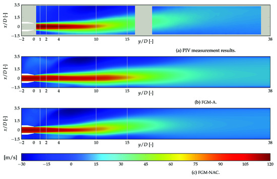
Figure 5.
Mean axial velocity.
Figure 6 shows profile plots of the axial velocity at several stream-wise locations along the combustor’s symmetry plane () for a more detailed image. The experimental data is visualised as a circle with lines to indicate the error margin as provided by Lammel et al. [2]. Again, overall, a very good agreement between simulation and experiment. The experimental results give a slightly higher velocity, though the overall shape of the profiles is very accurately described, for example the velocity gradient in the jet shear layer around . Here, the difference in the axial jet deceleration can be observed again. FGM-NAC provides the best agreement with the experiment. FGM-A overestimates the velocity from and onward. This is caused by an overprediction of the temperature and the consequent underprediction of the density. The plots furthermore show an overprediction of the negative velocity value in the recirculation zone.

Figure 6.
Mean axial velocity profiles plots at various stream-wise locations. FGM-NAC (–––), FGM-NA (– – –), FGM-A (−·−·−), Raman measurement results (∘) [2].
The mean transverse velocity , presented in Figure 7, shows a significantly larger difference between the models. This signifies a difference in the prediction of the size and location of the primary recirculation zone. For example, FGM-NAC shows a large negative velocity at , which indicates that the recirculation area is positioned more forward than in the other simulations. For all, however, it can be said that the transverse velocity magnitude is overpredicted in the recirculation zone. This can be attributed to the very large difference between axial and transverse momentum. The latter can jeopardise the assumption of isotropic turbulence made in the SST turbulence model. Downstream of the recirculation zone the simulations provide a better agreement with the experiments, with all models able to predict that the flame moves towards the centre.

Figure 7.
Mean transverse velocity profiles plots at various stream-wise locations. FGM-NAC (–––), FGM-NA (– – –), FGM-A (−·−·−), Raman measurement results (∘) [2].
4.2. Temperature Fields
Contour plots of the simulated mean temperature on the symmetry plane are shown in Figure 8b–d for FGM-A, FGM-NA and FGM-NAC, respectively. Figure 8a presents the experimental data as an average of the instantaneous shots, which is limited to a smaller region of the combustor (). A comparison of these plots points out a large difference between the simulation with non-adiabatic conditions and experimental data on one side and the adiabatic simulation on the other. In the case of adiabatic conditions, the temperature is not reduced by heat loss through the outer walls. This results in a mean maximum temperature of 2050 K, which corresponds to the adiabatic flame temperature at this equivalence ratio and inlet temperature. With the inclusion of heat loss through an isothermal wall boundary, a better agreement is found between simulations and experiment. This indicates the large effect of heat loss on the burner setup. Especially in the secondary recirculation zone behind the jet nozzle a large reduction in temperature can be seen, predicted well by the FGM simulations. FGM-NAC and FGM-NA yield maximum temperatures (1860 and 1890, respectively) close to the experimental value of 1850 K. However, the location of the maximum temperature is different in the simulations as opposed to the experiment. This can be attributed to the isothermal wall temperature condition; due to the large flow residence time in the primary recirculation zone around , the wall is expected to be heated by the flame through convective heat transfer. However, as the wall temperature is fixed, this heat transfer is exaggerated resulting in lower temperature values. It must be noted that due to the restricted region of available experimental data, it is not certain if the true maximum temperature is visible. It can be reasoned that further downstream, , a temperature higher than 1850 K is present in line with the nozzle centre line.
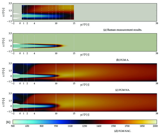
Figure 8.
Mean temperature on the symmetry plane.
In Figure 9 the profile plots of the temperature are shown. The temperature profiles indicate that heat loss indeed has significant effect for this combustor. The difference between adiabatic and non-adiabatic conditions is again very clear. Over the whole range, the heat loss reduces temperature by several hundred degrees Kelvin. Especially in the secondary recirculation zone the flow is cooled significantly. This can be seen at and is best represented by FGM-NAC. For the simulation follows the experiment very well. FGM-NA shows a steeper gradient at the jet shear layer as the tabulation does not incorporate the reduction of reaction rate due to heat loss. Interestingly, at , FGM-NA yields a lower temperature than the FGM-NAC. This might be caused by the change in shear layer break-up, which leads to a shorter primary recirculation area for the latter case. Therefore, a larger flow of hot exhaust gases reaches the upstream region of the recirculation area (which was also visible in the velocity profiles), resulting in a higher temperature locally. At downstream locations (), the temperature provided by the simulations deviates from the Raman spectroscopy results, with the simulations giving a shorter flame length characterised by the higher temperature inside the jet shear layer. This result was also observed in other RANS studies [8,11] and is said to be a result of underpredicted turbulent mixing at the shear layers. In instantaneous contour plots provided by LES [11] separated hot and cold pockets could be identified, which are a sign of a thickened flame. These unsteady pockets, which can only be produced by unsteady simulations, lead to conductive heat loss, reduced reaction rate and ultimately a thickened and longer flame. A last observation can be made at . Here, the minimum temperature obtained from the Raman experiment is higher than the specified inlet value, 630 K opposed to 573 K. This is too large to be the result from measurement inaccuracies and might indicate that reactions already start to take place at this location.
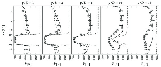
Figure 9.
Mean temperature profile plots at various stream-wise locations. FGM-NAC (–––), FGM-NA (– – –), FGM-A (−·−·−), Raman measurement results (∘) [2].
The temperature profile plots also show the effect of the velocity-pressure coupling and combined calculation of the density by the model (as density is directly linked to temperature with ideal gas law). The CFX solver uses a different approach for this than the original implementation of the model in Alya (Section 1). By comparing Figure 9 to the URANS temperature profiles reported in [11] it is found that results are almost identical for . For the locations further downstream, the current implementation is able to follow the experimental data better. Especially in the primary recirculation, the temperature is captured well by FGM-NAC, whereas the Alya solver results in a temperature of approximately 1400 K. Eventually at both studies obtain the same profile that is quantitatively and qualitatively incorrect. From this comparison it can be concluded that the FGM model is robust across solvers and turbulence treatments. Moreover, steady-state RANS provides almost identical results as compared to time-averaged URANS.
4.3. Heat Loss
From the contour and profile plots in Figure 8 and Figure 9 it was observed that a significant amount of the heat produced by the flame is lost through the wall boundary. This heat loss is a result of convective heat transfer following Newton’s law of heat transfer:
where the overall rate of convective heat loss is a function of the local heat transfer coefficient h, the surface (wall) temperature and the bulk temperature at some distance from the wall . However, since the velocity at the wall surface is zero due to the no-slip condition, the heat transfer directly at the wall is by conduction. This follows Fourier’s law:
with k the local fluid heat conductivity and n denoting the derivative with respect to the wall normal. Using this equation the total rate of heat loss through the wall is computed to be 3240 W. This result can be checked by assuming steady state and constant pressure and calculating the difference in ingoing and outgoing heat flow using the enthalpy:
This value for the heat loss is close to the estimated value of 3100 W computed in the Alya implementation of the model [14]. The small difference is satisfactory and might be the result of numerical errors in the implicit boundary condition for the temperature. This also again shows the consistency of the FGM model between Alya and CFX. The significance of this value for the heat loss can be made clear by comparing it to the thermal power of the combustor:
Here, LHV is the lower heating value of the fuel, being methane. This result shows that the heat lost to the combustor walls takes up 38% of the thermal power, which is a very large amount. Figure 10 shows a plot of the local heat transfer rate on the combustor wall boundary. A region of high heat loss can be identified, coinciding with the location of the recirculation zone. The fact that heat loss is large in this region was also predicted from the large gradients in the temperature profiles (Figure 9). There it was also observed that the high heat transfer results in a slight underprediction of the temperature in the recirculation area.

Figure 10.
Heat transfer through the outer wall.
4.4. Species Concentrations
Another property of interest is the mass or molar fraction of indicating species. These give more insight in the state of the reaction. The mass fraction of the steady state species are stored in a post-processing database. The molar fraction of species k can be computed from this as
with the molar mass of the mixture, , and species k, .
In Figure 11, Figure 12 and Figure 13 the molar fractions of the reacting species CH4, product H2O and intermediate species H2 are given. The first two plots show a good agreement between the simulations and experimental data. FGM-NAC shows the most spreading of the concentrations and gives the most accurate result. It can be noted that the maximum value of the methane molar fraction measured by the experiment is smaller than the unburnt mixture at this equivalence ratio ( = 0.0694, which is the value of the simulations). This indicates that reaction is already in progress, as was also mentioned in the discussion of the temperature profiles. Due to the underprediction of the flame length as described in Section 4.2, the simulations deviate from the experiment further downstream. At a significant amount of methane is still present according to the experiment which indicates that reaction is still in progress. The profile plots for H2O show a difference between experiment and simulations in the primary recirculation zone. The experiment again gives a lower molar fraction. A study using a detailed chemistry model by Di Domenico et al. [3] showed that burnt gases mix intensely with fresh gases in the shear layer. This can explain the lower concentration of H2O in the experimental data, opposed to the fully burnt mixture assumed by the simulations. This mixing effect can also be observed in the plots for the intermediate species H2 (Figure 13). Here, a very large discrepancy between experimental data and simulations is visible. Especially in the primary recirculation zone, where the experiment provides the largest molar fractions, it is noted that (fast) reactions not accounted for by the flamelet models affect the state of the flame. In other words, the equilibrium predicted by the chemistry tabulation is not equal to that shown by the experiments. Moreover, this effect cannot be attributed to the steady-state fluid flow modelling as unsteady simulations [11] showed the same distribution of species concentrations. It might rather be caused by the discrepancy between the FGM model assumptions and the flameless combustion regime, as will be discussed next.
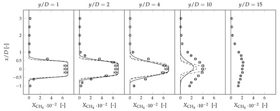
Figure 11.
Mean molar fraction of CH4 at various stream-wise locations. FGM-NAC (–––), FGM-NA (– – –), FGM-A (−·−·−), Raman measurement results (∘) [2].

Figure 12.
Mean molar fraction of H2O at various stream-wise locations. FGM-NAC (–––), FGM-NA (– – –), FGM-A (−·−·−), Raman measurement results (∘) [2].

Figure 13.
Mean molar fraction of H2 at various stream-wise locations. FGM-NAC (–––), FGM-NA (– – –), FGM-A (−·−·−), Raman measurement results (∘) [2].
4.5. Combustion Regime
A combustion regime diagram gives insight in the various regimes that a turbulent flame can reside in. To check whether the assumptions made in the derivation of the FGM model are valid, a scatter plot of all points in the fluid domain is mapped on the regime diagram and as result, the local flame regime can be estimated. For the plot, the laminar flame speed and flame thickness are based on the adiabatic flamelet solution calculated by Chemkin PREMIX, which is used in the FGM database. The laminar flame speed equals 0.068 m per second. The flame thickness is based on the definition using the temperature gradient [18]:
which yields a value of 3 × 10 m. The velocity fluctuations are estimated as and the integral turbulent length scale as . This gives the plot as shown in Figure 14. The diagram shows that the combustion falls mainly in the thickened flame regime. This result is in agreement with unsteady simulations on this burner configuration [9,10,11], where turbulence was seen to impact the combustion significantly. This result does mean that the assumption that the flame resides in the flamelet regime is not strictly valid. The plot must only be seen as an order of magnitude approximation, however. The definition of is based on isotropic turbulence, which is not accurate in the flame front. The regime of flameless combustion, which this setup is designed for, is normally associated with the distributed reaction zones area (top right of the diagram) [1]. The current simulation of the flame show data points that are in between the lines and , which is the transition zone between flamelet and distributed reaction zones. The contour and profile plots in the previous sections show that the model is able to predict velocity and temperature well. The FGM model in combination with the SST turbulence model provides satisfactory results for these variables. However, the flame length is underpredicted, and more specific to the FGM model the prediction of intermediate species concentrations in the recirculation area is poor. To accurately describe combustion in the flameless combustion regime using the FGM model an additional dimension in the flamelet generated manifold can be added as suggested by Huang et al. [19]. In this way flamelets at varying levels of flue gas dilution can be implemented in the chemistry tabulation. In combination with an extra control variable describing the vitiated recirculating gases, this can potentially improve the FGM model significantly in this regime.

Figure 14.
Regime diagram (as proposed by Peters [20]) with scatter based on FGM-NAC.
5. Conclusions
The effect of heat loss on the DLR jet burner setup is investigated. For this, the FGM combustion model by Gövert and Kok has been adapted for the use in Ansys CFX. This adaption has shown that the FGM model is robust across solvers and turbulence treatments. The model uses accurate laminar flame solutions stored in a chemistry database in combination with control variables to describe the local state of the flame. Three steady-state RANS simulations are performed with adiabatic conditions, isothermal wall boundaries with adiabatic chemistry tabulation and isothermal wall boundaries with heat loss included in the tabulation. The results are held against experimental data. From the comparison, the following conclusions can be drawn:
- The effect of heat loss on this configuration is shown to be prominent. The heat transfer through the wall is estimated to be 38% of the total thermal power. This is reflected in the results as the adiabatic simulation yields a maximum temperature of 2050 K, which is a significant overprediction of the measured value of 1850 K.
- However, the heat loss occurs mainly in the recirculation domains, which are large relative to the domain where chemical reaction occurs. In the limited domain where chemical reaction takes place, residence times are small and the heat loss is very small. Here the effect of heat loss is primarily due to mixing with cooled down recirculation gases. This has a modest effect on combustion chemistry.
- The effect of heat loss is demonstrated to be computed accurately on basis of convective and conductive heat loss for this non-luminous flame.
- While the velocity and temperature fields can be predicted accurately by the model, the species molar fractions show deviations from the experimental results in the recirculation area. From experiments the recirculating gases are known to mix with fresh gas. Therefore, a control variable representing vitiated recirculated gases may be beneficial for the representation of flameless combustion with FGM.
Author Contributions
Conceptualization, J.B.W.K.; methodology, J.W.H.; software, J.W.H.; validation, J.W.H.; formal analysis, J.W.H.; investigation, J.W.H.; resources, J.B.W.K. and A.G.K.; data curation, J.W.H.; writing—original draft preparation, J.W.H.; writing—review and editing, J.W.H. and J.B.W.K.; visualization, J.W.H.; supervision, J.B.W.K. and A.G.K.; project administration, J.B.W.K.; funding acquisition, J.B.W.K. All authors have read and agreed to the published version of the manuscript.
Funding
This research received no external funding.
Data Availability Statement
Simulation data can be found at https://doi.org/10.4121/18134045 (accessed on 4 July 2021).
Acknowledgments
We sincerely thank O. Lammel for providing the experimental data for comparison.
Conflicts of Interest
The authors declare no conflict of interest.
Abbreviations
The following abbreviations are used in this manuscript:
| CSP | Computational Singular Perturbation | DLR | German Aerospace Centre |
| FGM | Flamelet Generated Manifol | LES | Large Eddy Simulation |
| Probability Density Function | RANS | Reynolds-Averaged Navier-Stokes | |
| RPV | Reaction Progress Variable |
Appendix A. Database Generation
The adiabatic database is a two-dimensional manifold as a function of the reaction progress mean and variance . A single laminar flame is calculated using Chemkin PREMIX. To find a solution for the lean flame, a more rich flame () is used as a starting point and in consecutive calculations the equivalence ratio is reduced in steps of 0.02 to 0.71. The inlet temperature of this flame equals that of the simulation, i.e., 573 K. The laminar flame solution is employed in the CSP algorithm to define the b-vector for the mean reaction progress variable (Equation (1)). Subsequently, the properties are integrated using the presumed-PDF model. The turbulent manifold is stored for discretised points for the RPV mean and variance. For the mean a linear subdivision of 101 points is made. The reaction progress variance is discretised using a cubic division with 25 points, as the -PDF changes increasingly more for smaller values of the variance. The discretised point is defined as:
The turbulent database consequently consists of 2525 lines.
The non-adiabatic database uses multiple flamelet solutions as its basis, as mentioned in Section 2.1. A burner stabilised flame at is used as starting point and the equivalence ratio is reduced again in consecutive calculations until is reached. This first flamelet corresponds to adiabatic conditions with an inlet temperature of 573 K. Using this flamelet as initial guess, the second flame is calculated with a reduced reactants mass flow. This is continued until the lower enthalpy limit is reached. To describe the complete range of enthalpy accurately, a total of 40 flamelets is calculated and stored with corresponding value of . With the additional control variable the total number of lines in the database is increased to 101,000.
The properties stored in the database are shown in Table A1. A separate database contains the species mass fractions for post-processing.

Table A1.
Tabulated properties in the turbulent databases. For the adiabatic database equals unity.
Table A1.
Tabulated properties in the turbulent databases. For the adiabatic database equals unity.
References
- Perpignan, A.A.; Gangoli Rao, A.; Roekaerts, D.J. Flameless combustion and its potential towards gas turbines. Prog. Energy Combust. Sci. 2018, 69, 28–62. [Google Scholar] [CrossRef]
- Lammel, O.; Stöhr, M.; Kutne, P.; Dem, C.; Meier, W.; Aigner, M. Experimental Analysis of Confined Jet Flames by Laser Measurement Techniques. J. Eng. Gas Turbines Power 2012, 134, 041506. [Google Scholar] [CrossRef]
- Domenico, M.D.; Gerlinger, P.; Noll, B. Numerical Simulations of Confined, Turbulent, Lean, Premixed Flames using a Detailed Chemistry Combustion Model. In Proceedings of the ASME Turbo Expo 2011, Vancouver, BC, Canada, 6–10 June 2011. Number GT2011-45520. [Google Scholar]
- Bradley, D.; Kwa, L.; Lau, A.; Missaghi, M.; Chin, S. Laminar flamelet modeling of recirculating premixed methane and propane-air combustion. Combust. Flame 1988, 71, 109–122. [Google Scholar] [CrossRef]
- Sorrentino, G.; Ceriello, G.; de Joannon, M.; Sabia, P.; Ragucci, R.; van Oijen, J.; Cavaliere, A.; de Goey, L.P.H. Numerical Investigation of Moderate or Intense Low-Oxygen Dilution Combustion in a Cyclonic Burner Using a Flamelet-Generated Manifold Approach. Energy Fuels 2018, 32, 10242–10255. [Google Scholar] [CrossRef] [Green Version]
- Mayrhofer, M.; Koller, M.; Seemann, P.; Prieler, R.; Hochenauer, C. Evaluation of flamelet-based combustion models for the use in a flameless burner under different operating conditions. Appl. Therm. Eng. 2021, 183, 116190. [Google Scholar] [CrossRef]
- Perpignan, A.A.V.; Sampat, R.; Gangoli Rao, A. Modeling Pollutant Emissions of Flameless Combustion with a Joint CFD and Chemical Reactor Network Approach. Front. Mech. Eng. 2019, 5, 63. [Google Scholar] [CrossRef]
- Donini, A.; Martin, S.M.; Bastiaans, R.J.M.; van Oijen, J.A.; de Goey, L.P.H. Numerical Simulations of a Premixed Turbulent Confined Jet Flame Using the Flamelet Generated Manifold Approach with Heat Loss Inclusion. In Proceedings of the ASME Turbo Expo 2013, San Antonio, TX, USA, 3–7 June 2013. Number GT2013-94363. [Google Scholar]
- Fancello, A.; Panek, L.; Lammel, O.; Krebs, W.; Bastiaans, R.J.M.; de Goey, L.P.H. Turbulent Combustion Modeling using Flamelet-Generated Manifolds for Gas Turbine Applications in OpenFOAM. In Proceedings of the ASME Turbo Expo 2014, Düsseldorf, Germany, 16–20 June 2014. Number GT2014-26096. [Google Scholar]
- Proch, F.; Kempf, A.M. Modeling Heat Loss Effects in the Large Eddy Simulation of a Model Gas Turbine Combustor with Premixed Flamelet Generated Manifolds. Proc. Combust. Inst. 2015, 35, 3337–3345. [Google Scholar] [CrossRef]
- Gövert, S.; Mira, D.; Kok, J.B.W.; Vázquez, M.; Houzeaux, G. Turbulent Combustion Modelling of a Confined Premixed Jet Flame Including Heat Loss Effects Using Tabulated Chemistry. Appl. Energy 2015, 156, 804–815. [Google Scholar] [CrossRef]
- Houzeaux, G.; Vázquez, M.; Aubry, R.; Cela, J. A massively parallel fractional step solver for incompressible flows. J. Comput. Phys. 2009, 228, 6316–6332. [Google Scholar] [CrossRef]
- Smith, G.P.; Golden, D.M.; Frenklach, M.; Moriarty, N.W.; Eiteneer, B.; Goldenberg, M.; Bowman, C.T.; Hanson, R.K.; Song, S.; Gardiner, W.C.; et al. GRI-MECH 3.0. Available online: http://www.me.berkeley.edu/gri_mech/ (accessed on 4 July 2021).
- Gövert, S. Modelling the Effects of Heat Loss and Fuel/Air Mixing on Turbulent Combustion in Gas Turbine Combustion Systems. Ph.D. Thesis, University of Twente, Enschede, The Netherlands, 2016. [Google Scholar]
- Fiorina, B.; Baron, R.; Gicquel, O.; Thevenin, D.; Carpentier, S.; Darabiha, N. Modelling Non-Adiabatic Partially Premixed Flames Using Flame-Prolongation of ILDM. Combust. Theory Model. 2003, 7, 449–470. [Google Scholar] [CrossRef]
- McBride, B.J.; Gordon, S.; Reno, M.A. Coefficients for Calculating Thermodynamic and Transport Properties of Individual Species; Technical Memorandum 4513, NASA; 1993; Available online: https://shepherd.caltech.edu/EDL/PublicResources/sdt/refs/NASA-TM-4513.pdf (accessed on 4 July 2021).
- Menter, F.R. Two-equation Eddy-Viscosity Turbulence Models for Engineering Applications. AIAA J. 1994, 32, 1598–1605. [Google Scholar] [CrossRef] [Green Version]
- Poinsot, T.; Veynante, D. Theoretical and Numerical Combustion, 3rd ed.; Bordeaux, France; 2011; Available online: http://elearning.cerfacs.fr/combustion/onlinePoinsotBook/buythirdedition/index.php (accessed on 4 July 2021).
- Huang, X.; Tummers, M.; Roekaerts, D. Experimental and numerical study of MILD combustion in a lab-scale furnace. Energy Procedia 2017, 120, 395–402. [Google Scholar] [CrossRef]
- Peters, N. The turbulent burning velocity for large-scale and small-scale turbulence. J. Fluid Mech. 1999, 384, 107–132. [Google Scholar] [CrossRef]
Publisher’s Note: MDPI stays neutral with regard to jurisdictional claims in published maps and institutional affiliations. |
© 2022 by the authors. Licensee MDPI, Basel, Switzerland. This article is an open access article distributed under the terms and conditions of the Creative Commons Attribution (CC BY) license (https://creativecommons.org/licenses/by/4.0/).