Abstract
The phase-synchronized rotation of a pair of closely spaced vertical-axis wind turbines has been found in wind tunnel experiments and computational fluid dynamics (CFD) simulations. During phase synchronization, the two wind turbine rotors rotate inversely at the same mean angular velocity. The blades of the two rotors pass through the gap between the turbines almost simultaneously, while the angular velocities oscillate with a small amplitude. A pressure drop in the gap region, explained by Bernoulli’s law, has been proposed to generate the interaction torque required for phase synchronization. In this study, an analytical model of the interaction torques was developed. In our simulations using the model, (i) phase synchronization occurred, (ii) the angular velocities of the rotors oscillated during the phase synchronization, and (iii) the oscillation period became shorter and the amplitude became larger as the interaction became stronger. These observations agree qualitatively with the experiments and CFD simulations. Phase synchronization was found to occur even for a pair of rotors with slightly different torque characteristics. Our simulation also shows that the induced flow velocities influence the dependence of the angular velocities during phase synchronization on the rotation directions of the rotors and the distance between the rotors.
1. Introduction
A pair of closely spaced vertical-axis wind turbines (VAWTs) can yield more power than two isolated VAWTs [1]. This idea was extended to a wind farm where many pairs of small-sized VAWTs were placed in a limited area in order to yield a high power density [2]. VAWTs accept wind from all directions; thus, it is possible to place them in proximity to each other. In order to investigate the performance and characteristics of such closely spaced VAWTs, wind tunnel experiments [3,4,5,6,7,8] and computational fluid dynamics (CFD) simulations of a pair of VAWTs were performed in two dimensions [9,10,11,12,13,14], as well as in three dimensions [6,15].
In Refs. [4,5], wind tunnel experiments of a pair of two-bladed H-type Darrieus turbines were reported, and synchronization of the rotations was found in both counter-down (CD) and counter-up (CU) layouts. Note that, in the CD layout, the blades of the two rotors move in the downwind direction in the gap region between the rotors. In the CU layout, the blades move in the upwind direction in the gap region. It was found that the rotational speeds equalize and the power output increases. Let us call this phenomenon phase synchronization. It was also found that the phase difference between the rotors oscillates around a mean value, and converges to it during the phase synchronization period. However, the mechanism of phase synchronization was not discussed in their papers.
Jodai et al. performed wind tunnel experiments on a pair of closely spaced, small-sized rotors made by a 3D printer and found that phase synchronization occurs when the distance between the rotors is sufficiently small in the CD layout [7,8]. It was found that the rotational speed with phase synchronization was 13% greater than that for a single rotor under the extremely small gap condition; the gap distance was 10% of the rotor diameter. This was the first report on the steep rise of the rotational speed under phase synchronization of a pair of closely spaced VAWTs with the extremely small gap. The oscillation of the phase difference was not reported in their papers.
Hara et al. performed a two-dimensional CFD analysis [13,14] to simulate the experiments by Jodai et al. They adopted a dynamic fluid–body interaction (DFBI) model that enabled the angular velocities of the rotors to change dynamically. The simulation results showed that phase synchronization also occurred in the CFD analysis for both the CD and CU layouts. They also found that the angular velocities of the rotors oscillated around the mean value during phase synchronization. Note that the oscillation of the angular velocities around the mean value means the same as the oscillation of the phase difference. From the observations of the CFD simulation results, it was proposed that phase synchronization and the oscillation of the angular velocities occur because of the interaction torques generated by pressure fluctuations in the gap between the rotors. In fact, they found that the velocity increases and the pressure decreases according to Bernoulli’s law when blades of the two rotors come closer together in the gap region.
In this study, we developed an analytical model for the interaction torques that can be included in evolution equations of the angular velocities of rotors considered as solid bodies. Such a model is useful to understand the physics of the observed phenomena. Here, we present the details of the derivation, as well as numerical results showing the phase synchronization and the oscillation of the angular velocities. We also perform a simulation of a pair of rotors with slightly different torque characteristics and show that phase synchronization also occurs if interaction torques exist.
This paper is organized as follows. The details of the model, including the derivation of the interaction torques, are explained in Section 2. Then, Section 3 shows the numerical results based on the model. In particular, in Section 3.2, we report that the phase synchronization and oscillation of the angular velocities occur when using our model. We also report the dependence of the angular velocities in the phase synchronization regime on the gap in Section 3.3. The oscillations of the difference in angular velocities are shown in Section 3.4. The conclusions are given in Section 4. Appendix A shows the verification of our model based on comparison with CFD as well as experimental results, while Appendix B summarizes normalized expressions of our model.
2. Model
Let us consider a pair of VAWTs. The geometry of the layout is shown in Figure 1. The upstream wind flows from the left of the figure. The rotation directions of the rotors are shown by the arrows. Co-rotating, Counter Down, and Counter Up layouts are written as CO, CD, and CU, respectively. In the CD layout, the blades of the rotors move in the downwind direction in the gap region between the rotors. In contrast, in the CU layout, the blades move in the upwind direction.
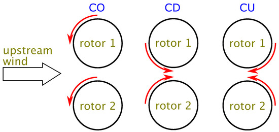
Figure 1.
Layouts of rotors.
Figure 2 explains the definitions of variables. The diameter and the radius of a rotor i are denoted by and , respectively. The gap between rotors i and j is given by . In this study, we only considered a pair of rotors. A rotor i has blades, and the position of a blade k is expressed as in the two-dimensional plane, of which the origin is at the center of rotor 1. An azimuthal angle of a blade k of a rotor i is expressed by , which is zero in the direction of the y axis and increases in the counterclockwise direction. The blades of a rotor are equally spaced in the azimuthal angle, and thus the angle between the neighboring blades is . The chord length and the area projected along the rotation direction of a blade k of a rotor i are denoted and , respectively.
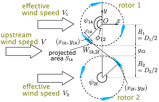
Figure 2.
Definitions of variables.
The distance between the blade k of the rotor i and the blade ℓ of the rotor j is written as , which varies in time due to the rotation. As we explain later in this section, we adopted a model to describe a change in the flow velocity according to the temporal change of , leading to a pressure fluctuation between the blades according to Bernoulli’s law. The center of the rotor j is in the direction of an angle seen from the center of rotor i. As with the azimuthal angle , the angle is also zero in the direction of the y axis and increases in the counterclockwise direction. The angle of the center of the rotor i seen from the center of the rotor j is , although only with and is shown in Figure 2.
The wind flows in the direction of the x axis. The upstream speed is denoted by V. The flow velocity experienced by the rotor differs for each rotor. The effective flow velocity immediately in front of rotor i is written as .
As mentioned above, we only considered a pair of rotors. The evolution equations governing the rotation are
where represent the two rotors, is the angular velocity, is the azimuthal angle of a representative blade, is the moment of inertia, is the rotor torque, is the load torque, and is the torque due to the interaction with the other rotor through pressure fluctuation in the gap between them. Note that is not necessarily but can be another with ; the meaning is the same for any choice of .
In the following section, we explain our torque models. First, we take the rotor torque as
This torque, without the last term , simulates the torque characteristics in the two-dimensional CFD by Hara et al., as shown in Figure 2 of Ref. [14]. Note that the rotor is operated at an angular velocity, in a sense of average over phase, where the torque in Equation (3) is balanced by a load torque introduced below. Since the balanced state occurs at an angular velocity larger than that at the maximum torque in the present choice of the load torque for a given flow velocity, the rotor torque characteristics at small angular velocity regime is not essential. Here, expresses a modulation in the rotor torque depending on the angle of the blades, which we explain shortly. Without this modulation, or setting , is a cubic function of for a given and takes a maximum value when on the positive side. When at the positive side, the rotor torque becomes zero. Thus, is sometimes called no-load angular velocity.
Here, we take
where and are constants. As shown in Appendix A, we chose these expressions by observing the CFD [13,14], as well as the experimental [7,8] data. The actual values used in our simulation are given in the next section. Note that normalized expressions of Equations (3)–(5), as well as equations to appear below are given in Appendix B, where it is shown that the normalized rotor torque is expressed by a tip–speed ratio for the rotor i and normalized and only.
The average of over is taken to be unity. As shown in Appendix A, it is known that the rotor torque by a single blade is finite at the upstream side and becomes maximal when a blade comes to the position . It decreases to almost zero at the downstream side when the rotor solidity is large. We assume that
for a single blade. Figure 3 shows the azimuthal angle dependence of . In the figure, plots Equation (6). The curve of plots a summation of the modulation function for over three blades equally spaced in the azimuthal angle and normalized such that . Note that the function for the modulation can be rather flexibly chosen since it is enough to simulate qualitative aspects of the torque modulation. Any function with its maximum at and almost zero in the downstream half may be acceptable.
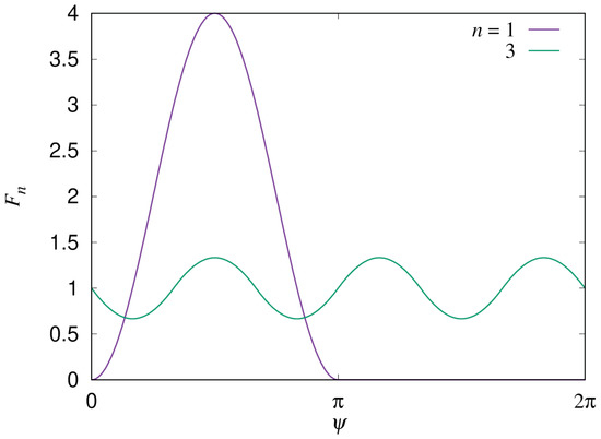
Figure 3.
Modulation function of the rotor torque on the azimuthal angle of the blade. The curves and plot the modulation for a single blade and a summation over three blades, respectively. The average of over is taken to be unity.
For the effective wind speed, we use
where is a coefficient of self-induced velocity, and is the circulation of rotor j. The second term expresses the velocity induced by another rotor. This assumption, assigning a circulation for a rotor, is similar to the one in Ref. [16]. We take
where is a constant. This dependence was also obtained by the CFD results as shown in Appendix A. By using the effective wind speed , the rotor torque on rotor i can be calculated. Note that in Equation (7), especially its mutually induced velocity in the second term of the right-hand side, is evaluated by using the coordinate of the center of rotor i. In reality, the effective flow velocity is different for each blade, and the summation of the torques on every blade of a rotor determines the rotor torque. However, in this study, the effective velocity is used for calculating the rotor torque as an average of the effective velocities for all blades in the rotor, and we assume that is the flow velocity immediately in front of rotor i. Instead of considering the torques on each blade, we take into account the torque modulation of the rotor torque via . The modulation expresses the fact that the blade experiences significantly smaller flow than the upstream when it is in the downstream half of the rotation.
Secondly, we take the load torque as
The dependence, square of angular velocity, is known as the ideal load torque to obtain highest power at each instance [17]. The CFD simulations by Hara et al. [13,14] also adopted the ideal load torque of the same form. Within our torque model, it is shown that the load torque in Equation (9) works to keep the highest power as follows. According to the rotor torque in Equation (3), the power takes a maximum value when , and the corresponding rotor torque is . By using Equations (4) and (5), these are written such that the maximum power is obtained when and the corresponding torque is . The ideal operation of the turbine is achieved by balancing the rotor torque by the load torque for whatever . This is realized by setting , which is obtained by eliminating in Q by using . The coefficient is determined so that the load torque takes 95% of when the power becomes maximal for a given in Section 3.1.
Finally, we come to the torque caused by pressure fluctuations between the blades. The positions of the blades of rotors 1 and 2 are given by
The distance between two blades at and is
Here, we consider the flow to be incompressible and assume that
where is the average flow velocity, and expresses the change in the flow velocity between the two blades due to a change in distance between them. Note that the calculation of may be improved by taking not only the x component of the flow velocity but also the y component, or taking the distance in the y direction between the blades k and ℓ instead of the distance itself. Let us leave this refinement as a future issue. We roughly estimate the change of velocity in this study. Then, we obtain the pressure fluctuation using Bernoulli’s law
as
Here, the air pressure is written as p. Note that we neglected the effects of viscous force and unsteadiness of the flow. We adopted the Bernoulli’s law to explain interactions between the blades due to pressure fluctuation through the increase in the flow velocity in the x direction observed in the CFD results, as shown in Figure 20 of Ref. [14]. The force on a blade due to this pressure fluctuation is calculated by integrating with the blade volume. The necessary force component is that along the rotation direction for the blade k of the rotor i. As an example, for , this is calculated as
By using Equation (15),
Then, we can obtain
The torque on a blade due to pressure fluctuations may be approximated by multiplying the blade volume by the rotor radius . Now, we also assume that the total torque on a rotor can be obtained by adding contributions from all blades. Then, we obtain
Here, a coefficient is included to control the strength of the interaction between the blades due to the pressure fluctuation, since the summation over all blades may be rather rough. Readers may think that it is strange to add a contribution from a blade at the opposite side of the gap between the rotors; it is natural to count only contributions from blades in the gap region. We also considered a model where rotors are taken as solid cylinders and only considered a narrowed channel between the gap region. This may not be a bad choice for high solidity rotors; however, the flow goes into the region surrounded by the blades of a rotor in reality. Thus, we decided to consider all combinations of blades and to add contributions from all pairs of blades in our model as an average in a sense, although big contributions must arise when two blades come to the gap region, and thus, other contributions may not play major roles. From a numerical computation viewpoint, this assumption, summation over all blades, is far simpler than taking the azimuthal angle of each blade into account to judge whether we should add its contribution or not. The on/off nature of the contributions can yield abrupt changes in torque, leading to a strange time evolution. Thus, we avoid this confusion.
3. Numerical Results
3.1. Characteristics of Rotors
We only consider a pair of rotors and assume that they have completely the same characteristics, except when otherwise stated. The following parameters are chosen. These are the same as those used in the CFD simulations in [13], Hara et al. [14]. The number of blades per rotor is . The radius of the rotor is . The chord length is , and the area projected along the rotation direction is for . The moment of inertia is . Note that the previous CFD simulation [13,14] was two-dimensional, where the rotor height was instead of , as used for the three-dimensional model, and the moment of inertia was set at .
From the CFD simulation for a single rotor with the above parameters, under a fixed angular velocity condition, it was found that the maximum power is obtained when for . The time-averaged rotor torque in this case is . By using these values, we determined and for the rotor torque, Equation (3), and for the load torque, Equation (9). We further determined that and from and via Equations (4) and (5).
In the case of our rotor torque (3), the power becomes maximal at for a given . The rotor torque at this angular velocity is . We chose this to match the CFD value . Therefore, it is assumed that and . From Equation (4), we determine that
Additionally, from Equation (5), we obtain
Furthermore, in the CFD simulation, the angular velocity becomes stationary when the load torque is chosen to be 95% of the optimum rotor torque. We assume the same and thus obtain
We will set the value of in Section 3.3.
By using these parameters, we obtain the torque curves shown in Figure 4. The rotor torque is plotted for and without considering the modulation by and the induced velocities. Note that the rotor torque characteristics at angular velocities lower than the maximum torque for each V are assumed to be different from those of the CFD and the experimental wind turbines to simplify the analysis. The intersection of the rotor torque curve for a given flow velocity and the load torque curve is the a stable steady state. For example, is the angular velocity at the steady state when . Note that the angular velocity at the steady state for a given flow velocity does not change when the rotor torque Q or is multiplied by a constant factor, since the load torque L was chosen to also be multiplied by the same factor in the present study.
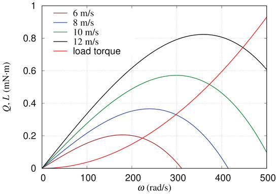
Figure 4.
The rotor torques for , and and load torques are plotted against the angular velocity of the rotor.
Note that the adopted angular velocity values (3500 rpm) and the torque at the maximum power are slightly different from the values at the steady state (3496 rpm) and obtained in the CFD simulation based on the DFBI for a single rotor [14]. “SI” stands for single. We can use these values of and instead of those used above to determine , and and then and via Equations (4) and (5) by assuming the following three conditions: (i) the rotor torque balances the load torque at , (ii) the balanced torque is , and (iii) is 95% of the torque at the maximum power. We can immediately obtain or from the second condition and from the third condition, respectively. We can also obtain from the first one, which becomes a cubic equation for for a given . The resulting values are , , and , of which relative differences from the values obtained in Equations (24)–(26) and used in the simulations presented in Section 3.2,Section 3.3,Section 3.4 are within 5%. Note that was calculated from the cubic equation by a perturbation technique based on a trivial approximate solution that gives the maximum power in our model.
3.2. Phase Synchronization
In this Section 3.2, we demonstrate that phase synchronization occurs due to the interaction torque generated by the pressure fluctuation. In order to focus on the effect of the interaction torque, we set and , so that , i.e., the effective flow velocity is the same as the upstream flow velocity. The upstream velocity used in this section is . Furthermore, we set to exclude the effects of torque modulation due to the azimuthal angle of the blade.
We solve the evolution Equations (1) and (2) for by the fourth-order Runge–Kutta method. The step size is , where . Average of initial angular velocities
Figure 5 shows the time evolution of for , and in the CD layout. The gap between the rotors is . The initial conditions are , , , and . The initial angular velocities have different magnitudes. One of the blades of rotor 1 is at the narrowest position in the gap initially and that of rotor 2 is slightly ahead.
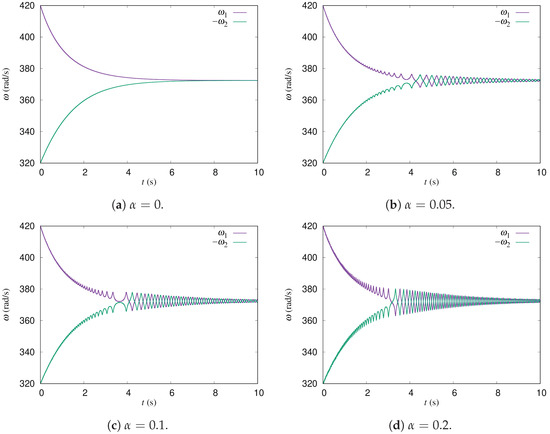
Figure 5.
Time evolution of for , and in the CD layout with a gap.
When , the rotors just reach their individual steady states since there is no interaction between the rotors. The rotors have identical characteristics, and thus they rotate at the same angular velocity at the steady state.
When is finite, the angular velocities oscillate. This simulates the phase synchronization observed in the experiments as well as in the CFD simulations. Such phase synchronization and oscillation of phase difference in the wind tunnel experiments of a pair of two-bladed H-type Darrieus turbines were reported in Section 6.2 of Ref. [4] and in Section 4.4 of Ref. [5]. The phase synchronization and the oscillation of angular velocities in the two-dimensional CFD were reported in Section 3.5 and Figure 17–19, of Ref. [14]. The oscillation period becomes shorter as increases since the interaction between the rotors becomes stronger. The oscillation period of the angular velocities is about for at , while it is about for . Moreover, the oscillation period becomes shorter over time.
The oscillation amplitude of the angular velocity becomes larger as is increased. This is also because the interaction becomes stronger as is increased.
Figure 6 shows the time evolution of the phase differences when and . The index k takes a value of , or 3. Before the phase synchronization, runs over the whole range of azimuthal angles. During phase synchronization, on the other hand, oscillates around a fixed angle. One of the three blades of rotor 2 has a phase difference of with blade 1 of rotor 1, which means that those blades meet in the gap region every rotation. We see that the oscillation period of the angular velocity during phase synchronization is shorter for larger values, as shown in Figure 6. Moreover, the phase synchronization starts earlier for larger values.
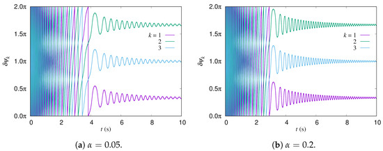
Figure 6.
Time evolution of phase differences for and in the CD layout with gap.
Phase synchronization occurs also in the CU layout. Since the induced velocity is not taken into account in the simulations presented in this section, the oscillation period and amplitude are the same as those in the CD layout.
Surprisingly, phase synchronization also occurs in the CO layout. The time evolution of for and is shown in Figure 7. Compared with the data presented in Figure 5 for the CD layout, the oscillation period of the angular velocities of the CO layout is longer than those of the CD layout with the same values. We can also see that the oscillation amplitude of the angular velocities is smaller in the CO layout than that in the CD layout. This is of course because the interaction in the CO layout is much weaker than in the CD and CU layouts. In this simulation, the characteristics of the rotors are identical, and thus, the angular velocity is the same at the steady state without the interaction. In the beginning, the magnitudes of and are largely different. Thus, they have almost no interaction. However, as the magnitudes of and become closer to their steady-state values, the time period that the blades of the rotors stay in the narrow gap region together becomes longer, although it must still be much shorter than that for the CD and CU layouts. This makes the interaction effect visible, even in the CO layout.
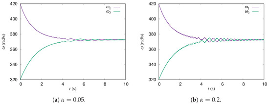
Figure 7.
Time evolution of for and in the CO layout with gap. Induced velocities are not taken into account.
In fact, it becomes difficult for phase synchronization to occur if the angular velocities of the rotors at steady state without interaction are different from each other. We set the rotor torque of rotor 2 as 95% of that of rotor 1 while keeping the load torque unchanged. The other parameters are the same as those used in Figure 7. This makes the angular velocity of rotor 2 about at its steady state without interaction, which is about 1.7% smaller than that of rotor 1. The time evolution of for is plotted in Figure 8a. Phase synchronization does not occur in this case. The angular velocities oscillate around each steady-state value. Note that phase synchronization occurs when , even in this case.
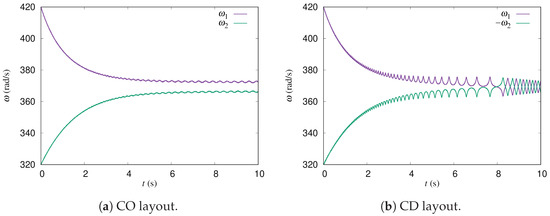
Figure 8.
Time evolution of for the (a) CO and (b) CD layouts with and when the rotor torque of rotor 2 is 95% that of rotor 1. The induced velocities are not taken into account.
On the other hand, phase synchronization occurs for the CD layout, even at , which is shown in Figure 8b. The angular velocity of the rotors during phase synchronization is about , which is about an average of the natural values of the two rotors without interaction. Phase synchronization occurs for smaller interactions because the relative speed of the blades of the two rotors is smaller for the CD layout than for the CO layout, leading to a longer interaction duration.
It may be worth pointing out that can be used to qualitatively reproduce the parameter dependence of the experimental and CFD results on aspects such as the solidity and upstream flow velocity by assuming that is dependent on these parameters. This is left as a future issue.
3.3. Dependence of the Synchronized Angular Velocity on the Gap
In this Section 3.3, we focus on the dependence of the synchronized angular velocity on the gap, especially when we take into account the mutually induced velocities generated by each component. Therefore, we set according to the CFD simulation results [13,14]. The sign of is positive when and negative when . On the contrary, we set , since the self-induced velocity by the rotor itself should be the same for identical rotors. When , the effect is only a change in the upstream velocity by a factor of for both rotors. Note that the torque modulation in Equation (3) with is taken into account in the results presented in this section.
The angular velocity at steady state is plotted against the gap width in Figure 9. Each angular velocity is obtained using the Fourier transform of the time series data at the steady state. We show the results for , although they are the same for different values. Additionally, just introduces modulation of the angular velocity, of which the period is one-third of the rotation period of the rotor and does not affect the phase-synchronized angular velocity.
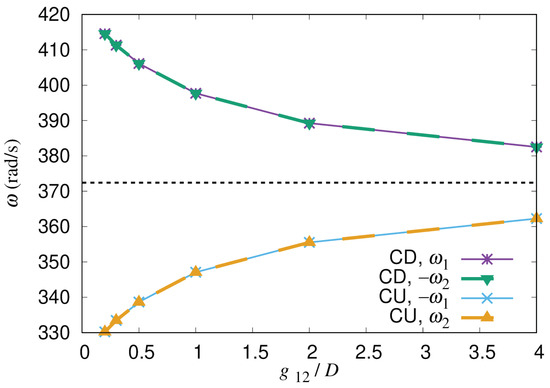
Figure 9.
The angular velocity in the phase-synchronized steady state is plotted against the gap . The dashed line around shows the angular velocity at the steady state without the mutually induced velocity.
The magnitudes of the angular velocities and agree well in both the CD and CU layouts. The dashed line at is the angular velocity without the mutually induced velocity. The angular velocities at each are larger (smaller) than this value in the CD (CU) layout. This is due to the induced velocity. The effective velocity is larger (smaller) than the upstream velocity in the CD (CU) layout, as found in the CFD simulation [13,14]. Furthermore, the angular velocity increases (decreases) as the gap is narrowed in the CD (CU) layout because the magnitude of the induced velocity becomes larger for smaller gaps. This dependence can be clearly observed for the CD layout in the experiments [7,8] and the CFD simulations, except for the small gap distances [13,14]. For the CU layout, on the other hand, further analysis is required for comparison with the experiments and the CFD simulations.
3.4. Oscillation Period of the Difference in Angular Velocities
In this Section 3.4, we analyze the oscillation period of the difference of angular velocities . The parameters used are the same as those in Section 3.3. Figure 10 shows the time evolution of for the CD and CU layouts with and . The parameter was chosen to control the interaction strength for which the oscillation period of has a comparable order of magnitude with the experiments [4,5] and the CFD simulations [13,14]. The difference oscillates around 0 during phase synchronization and decays gradually. The oscillation period becomes shorter as time proceeds in all cases, as shown in Figure 10.
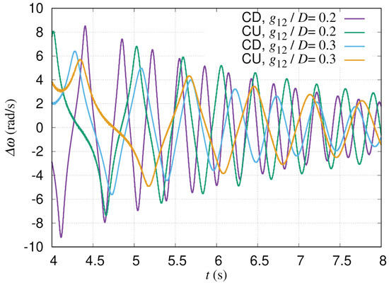
Figure 10.
Time evolution of difference of angular velocities is shown. The oscillation period is longer for larger gap distances, as well as for the CU layout compared with the CD layout.
First, we found that the oscillation period is longer for the CU layout than the CD layout if the gap distance is the same. For example, the oscillation period is about 0.36 s for the CD layout with at around s, while it is about 0.55 s for the CU layout.
Second, we found that the oscillation period is longer for a larger gap distance for a given layout. For example, the oscillation period is about 0.36 s when for the CD layout at around s, while it is about 0.62 s when .
The oscillation period of seems to be related to the mean angular velocity during phase synchronization; is longer for smaller mean angular velocities. The mean angular velocity is smaller in the CU layout than in the CD layout because of the mutual induced velocity (see Figure 9). Additionaly, the interaction becomes weaker if the gap distance is larger, thereby the oscillation period becomes longer.
Note that it is difficult to find such trends for the amplitude of , since it decays over time. However, we found that the decay is slower for the CU layout than the CD layout if the gap distance is the same. The damping rate seems to be smaller for longer oscillation periods. The oscillation amplitude for the CD layout with is about 7 rad/s at around s. The relative magnitude for the mean angular velocity rad/s is about 1.7%. The relative magnitude is a bit larger for the CU layout, since the mean angular velocity is smaller while the oscillation amplitude is comparable if the gap distance is the same.
4. Conclusions
We developed an analytical model of the interaction torque between two vertical-axis wind turbines through pressure fluctuation. In this model, the pressure fluctuation is obtained according to Bernoulli’s law, taking into account the temporal change in distance between the blades. Although rather crude assumptions were made in the development of the model, our simulations successfully demonstrated the phase synchronization as well as the oscillation of angular velocities around the mean value observed in the experiments and CFD simulations.
Our simulation results show that the angular velocities of the rotors oscillate in time during phase synchronization. When an artificial parameter is changed to strengthen the interaction, the oscillation period becomes shorter and the amplitude becomes larger. This is reasonable physically.
It was also found that phase synchronization occurs even for a pair of rotors with slightly different torque characteristics. This is important because the characteristics of the rotors cannot be identical in experiments.
Our model includes the induced velocities, which change the effective wind speed at each rotor. The simulation results also show that the mutually induced velocity can explain the qualitative dependence of the phase-synchronized angular velocities on the rotational direction of the rotors and the gap distance between them.
The oscillation period of the difference in angular velocities was found to be longer in the CU layout than in the CD layout. Additionally, the oscillation period was found to be longer for larger gap distances. This dependence seems to be related to the mean angular velocity of the rotors during phase synchronization. The mutually induced velocity changed the mean angular velocity in our simulations. The weaker interaction for larger gap distance made the oscillation period longer.
Author Contributions
Conceptualization, M.F., Y.H. and Y.J.; methodology, M.F.; software, M.F.; validation, Y.H. and Y.J.; formal analysis, M.F.; investigation, M.F.; resources, M.F.; data curation, M.F.; writing—original draft preparation, M.F.; writing—review and editing, Y.H. and Y.J.; visualization, M.F.; supervision, Y.H.; project administration, Y.H. and Y.J.; funding acquisition, Y.H. and Y.J. All authors have read and agreed to the published version of the manuscript.
Funding
This work was supported by JSPS KAKENHI Grant Number JP18K05013. The second author was supported in part by the International Platform for Dryland Research and Education (IPDRE), Tottori University.
Institutional Review Board Statement
Not applicable.
Informed Consent Statement
Not applicable.
Data Availability Statement
The data presented in this study are available from the corresponding author upon reasonable request.
Conflicts of Interest
The authors declare no conflict of interest.
Nomenclature
| Diameter of rotor i | |
| Radius of rotor i | |
| Gap between rotors i and j | |
| Number of blades on rotor i | |
| x | Coordinate in streamwise direction |
| y | Coordinate in spanwise direction |
| x coordinate of blade k of rotor i | |
| y coordinate of blade k of rotor i | |
| Azimuthal angle of blade k of rotor i | |
| Chord length of blade k of rotor i | |
| Projected area of blade k of rotor i along rotation direction | |
| Distance between blade k of rotor i and blade ℓ of rotor j | |
| Angle of rotor j observed from rotor i | |
| V | Upstream flow speed |
| Effective flow velocity at rotor i | |
| Moment of inertia of rotor i | |
| Angular velocity of rotor i | |
| Rotor torque on rotor i | |
| Load torque on rotor i | |
| Torque due to pressure fluctuation on rotor i | |
| Azimuthal angle of representative blade of rotor i | |
| Maximum rotor torque for given | |
| No-load angular velocity for given | |
| Torque-modulation function for n-blades rotor | |
| Parameter for | |
| Parameter for | |
| Tip-speed ratio of rotor i | |
| Azimuthal angle fixed in space | |
| Solidity of rotor i | |
| Torque-modulation function for single-blade rotor | |
| Parameter for self-induced velocity | |
| Circulation of rotor j | |
| Parameter for | |
| Parameter for | |
| Average flow velocity | |
| Change in flow velocity | |
| Pressure fluctuation | |
| p | Air pressure |
| Parameter controlling strength of interaction between rotors | |
| Steady-state angular velocity of single rotor by CFD using DFBI model | |
| Steady-state rotor torque of single rotor by CFD using DFBI model | |
| Average of initial angular velocities | |
| Phase differences between representative blade of rotor 1 and blade k of rotor 2 | |
| Difference of angular velocities | |
| Torque coefficient of rotor i | |
| Normalized maximum rotor torque | |
| No-load tip-speed ratio | |
| Mass density of air | |
| Swept area of rotor i | |
| Normalized circulation of rotor j | |
| Normalized load torque for rotor i | |
| Parameter for |
Appendix A. Verification of Parameter Dependence
In this Appendix A, CFD and experimental data to determine dependence of on flow velocity V in Equation (4), dependence of on V in Equation (5), CFD data to determine expression of the torque-modulation function in Equation (6), and dependence of on V in Equation (8) are shown.
First, let us show the dependence of on flow velocity V read from Figure 2 of Ref. [14] and Figure 3 of Ref. [8]. Figure A1 shows the CFD and experimental data, as well as their fitting curves taken to be quadratic in V. The fitting curves agree well with the CFD and experimental data.
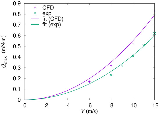
Figure A1.
from Figure 2 of Ref. [14], Figure 3 of Ref. [8], and their fitting curves are shown.
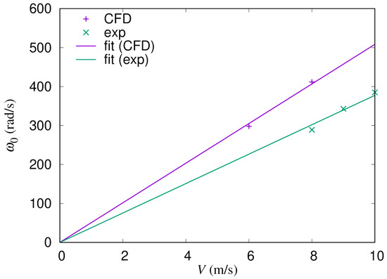
Second, let us show the dependence of on flow velocity V, also read from Figure 2 of Ref. [14] and Figure 3 of Ref. [8]. Figure A2 shows the CFD and experimental data, as well as their fitting curves taken to be linear in V. Although the number of data points is not enough, the fitting curves appear to agree well with the CFD and experimental data.
Third, the torque dependence on the azimuthal angle obtained by the CFD is shown. A rotor with three blades, of which dimensions are the same as described in Section 3.1, was placed in the flow field of which upstream flow velocity was 10 m/s. The modulation of the torque, expressed by Equation (6), tries to simulate this dependence. Figure A3 shows the averaged torques over the 16th–20th rotations of the CFD data, which was not published previously. For , the torque is the summation of torques on all blades of the rotor. The torque for a single blade has its maximum at . In the downstream half, the torque on a single blade becomes negative in the CFD, although it is set to be zero in Equation (6) for simplicity.
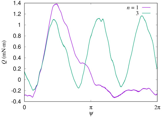
Figure A3.
Torque dependence on the azimuthal angle obtained by CFD. Equation (6) tries to simulate this dependence.
Finally, let us show the dependence of on flow velocity. Figure A4 shows obtained by CFD simulations, and their fitting curves taken to be linear in flow velocity. The CFD data were obtained by the time average of the simulation results. In the figure, “inf” means a plot of asymptotic values of at infinity against upstream flow speeds, and the “ep”, or evaluation point, means a plot of evaluated on a circle with a 36.1 mm radius centered at the rotor against flow speeds on the upstream side at 36.1 mm from the rotor center. Precisely, the flow speeds of the “ep” case are obtained by averaging over a 50 mm range in the spanwise direction. Note that the horizontal axis is not the upstream velocity for the “ep” case, although it is labeled by V. The fitting curves agree well with the CFD data.
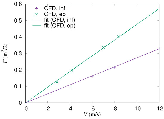
Figure A4.
obtained by CFD results and the fitting curves are shown.
Appendix B. Normalized Expression
In this Appendix B, normalized expressions of our model are summarized. First, let us normalize and given in Equations (4) and (5), respectively, as follows:
where is the mass density of air, and is the swept area of rotor i. Note that and are independent of . By using Equations (A1) and (A2), the torque coefficient , or normalized rotor torque given in Equation (3) with , can be expressed as
where is the tip–speed ratio of rotor i. The torque coefficient is expressed only by , and the dimensionless parameters and only. The rotor torque becomes zero when becomes equal to the no-load tip–speed ratio .
Next, the circulation in Equation (8) is normalized as
Note that is independent of .
Again, the parameter is independent of .
By using these expressions, numerical values of , , , and corresponding to the parameters used in Section 3 are obtained as follows:
Note that the mass density of air is assumed to be . The rotor radius is and the swept area is .
Let us point out that the simulation results shown in Section 3 can be interpreted, if is expressed by the tip–speed ratio , as results with a different set of a flow velocity , a rotor radius , and a swept are that give the same dimensionless parameters , , , and .
References
- Thomas, R.N. Coupled Vortex Vertical Axis Wind Turbine. US Patent US 6,784,566 B2, 31 August 2004. [Google Scholar]
- Dabiri, J.O.; Greer, J.R.; Koseff, J.R.; Moin, P.; Peng, J. A new approach to wind energy: Opportunities and challenges. AIP Conf. Proc. 2015, 1652, 51–57. [Google Scholar] [CrossRef] [Green Version]
- Ahmadi-Baloutaki, M.; Carriveau, R.; Ting, D.S.K. A wind tunnel study on the aerodynamic interaction of vertical axis wind turbines in array configurations. Renew. Energy 2016, 96, 904–913. [Google Scholar] [CrossRef]
- Vergaerde, A.; De Troyer, T.; Kluczewska-Bordier, J.; Parneix, N.; Silvert, F.; Runacres, M.C. Wind tunnel experiments of a pair of interacting vertical-axis wind turbines. J. Phys. Conf. Ser. 2018, 1037, 072049. [Google Scholar] [CrossRef]
- Vergaerde, A.; De Troyer, T.; Standaert, L.; Kluczewska-Bordier, J.; Pitance, D.; Immas, A.; Silvert, F.; Runacres, M.C. Experimental validation of the power enhancement of a pair of vertical-axis wind turbines. Renew. Energy 2020, 146, 181–187. [Google Scholar] [CrossRef]
- Jiang, Y.; Zhao, P.; Stoesser, T.; Wang, K.; Zou, L. Experimental and numerical investigation of twin vertical axis wind turbines with a deflector. Energy Convers. Manag. 2020, 209, 112588. [Google Scholar] [CrossRef]
- Jodai, Y.; Hara, Y.; Sogo, Y.; Marusasa, K.; Okinaga, T. Wind tunnel experiments on interaction between two closely spaced vertical axis wind turbines. In Proceedings of the 23rd Chu-Shikoku-Kyushu Branch Meeting, The Japan Society of Fluid Mechanics, Yamaguchi, Japan, 1–2 June 2019; pp. 11-1–11-2. [Google Scholar]
- Jodai, Y.; Hara, Y. Wind Tunnel Experiments on Interaction between Two Closely Spaced Vertical-Axis Wind Turbines in Side-by-Side Arrangement. Energies 2021, 14, 7874. [Google Scholar] [CrossRef]
- Zanforlin, S.; Nishino, T. Fluid dynamic mechanisms of enhanced power generation by closely spaced vertical axis wind turbines. Renew. Energy 2016, 99, 1213–1226. [Google Scholar] [CrossRef] [Green Version]
- Chen, W.H.; Chen, C.Y.; Huang, C.Y.; Hwang, C.J. Power output analysis and optimization of two straight-bladed vertical-axis wind turbines. Appl. Energy 2017, 185, 223–232. [Google Scholar] [CrossRef]
- De Tavernier, D.; Ferreira, C.; Li, A.; Paulsen, U.S.; Madsen, H.A. Towards the understanding of vertical-axis wind turbines in double-rotor configuration. J. Phys. Conf. Ser. 2018, 1037, 022015. [Google Scholar] [CrossRef] [Green Version]
- Ma, Y.; Hu, C.; Li, Y.; Li, L.; Deng, R.; Jiang, D. Hydrodynamic Performance Analysis of the Vertical Axis Twin-Rotor Tidal Current Turbine. Water 2018, 10, 1694. [Google Scholar] [CrossRef] [Green Version]
- Hara, Y.; Jodai, Y.; Okinaga, T.; Sogo, Y.; Kitoro, T.; Marusasa, K. A synchronization phenomenon of two closely spaced vertical axis wind turbines. In Proceedings of the 25th Chu-Shikoku-Kyushu Branch Meeting, The Japan Society of Fluid Mechanics, Takamatsu, Japan, 31 May 2020; pp. 3-1–3-2. [Google Scholar]
- Hara, Y.; Jodai, Y.; Okinaga, T.; Furukawa, M. Numerical Analysis of the Dynamic Interaction between Two Closely Spaced Vertical-Axis Wind Turbines. Energies 2021, 14, 2286. [Google Scholar] [CrossRef]
- Jin, G.; Zong, Z.; Jiang, Y.; Zou, L. Aerodynamic analysis of side-by-side placed twin vertical-axis wind turbines. Ocean Eng. 2020, 209, 107296. [Google Scholar] [CrossRef]
- Whittlesey, R.W.; Liska, S.; Dabiri, J.O. Fish schooling as a basis for vertical axis wind turbine farm design. Bioinspir. Biomimetics 2010, 5, 035005. [Google Scholar] [CrossRef] [PubMed] [Green Version]
- Novak, P.; Ekelund, T.; Jovik, I.; Schmidtbauer, B. Modeling and control of variable-speed wind-turbine drive-system dynamics. IEEE Control Syst. Mag. 1995, 15, 28–38. [Google Scholar] [CrossRef]
Publisher’s Note: MDPI stays neutral with regard to jurisdictional claims in published maps and institutional affiliations. |
© 2022 by the authors. Licensee MDPI, Basel, Switzerland. This article is an open access article distributed under the terms and conditions of the Creative Commons Attribution (CC BY) license (https://creativecommons.org/licenses/by/4.0/).