Analytical Model for Phase Synchronization of a Pair of Vertical-Axis Wind Turbines

Abstract

The phase-synchronized rotation of a pair of closely spaced vertical-axis wind turbines has been found in wind tunnel experiments and computational fluid dynamics (CFD) simulations. During phase synchronization, the two wind turbine rotors rotate inversely at the same mean angular velocity. The blades of the two rotors pass through the gap between the turbines almost simultaneously, while the angular velocities oscillate with a small amplitude. A pressure drop in the gap region, explained by Bernoulli’s law, has been proposed to generate the interaction torque required for phase synchronization. In this study, an analytical model of the interaction torques was developed. In our simulations using the model, (i) phase synchronization occurred, (ii) the angular velocities of the rotors oscillated during the phase synchronization, and (iii) the oscillation period became shorter and the amplitude became larger as the interaction became stronger. These observations agree qualitatively with the experiments and CFD simulations. Phase synchronization was found to occur even for a pair of rotors with slightly different torque characteristics. Our simulation also shows that the induced flow velocities influence the dependence of the angular velocities during phase synchronization on the rotation directions of the rotors and the distance between the rotors.

1. Introduction

A pair of closely spaced vertical-axis wind turbines (VAWTs) can yield more power than two isolated VAWTs [1]. This idea was extended to a wind farm where many pairs of small-sized VAWTs were placed in a limited area in order to yield a high power density [2]. VAWTs accept wind from all directions; thus, it is possible to place them in proximity to each other. In order to investigate the performance and characteristics of such closely spaced VAWTs, wind tunnel experiments [3,4,5,6,7,8] and computational fluid dynamics (CFD) simulations of a pair of VAWTs were performed in two dimensions [9,10,11,12,13,14], as well as in three dimensions [6,15].

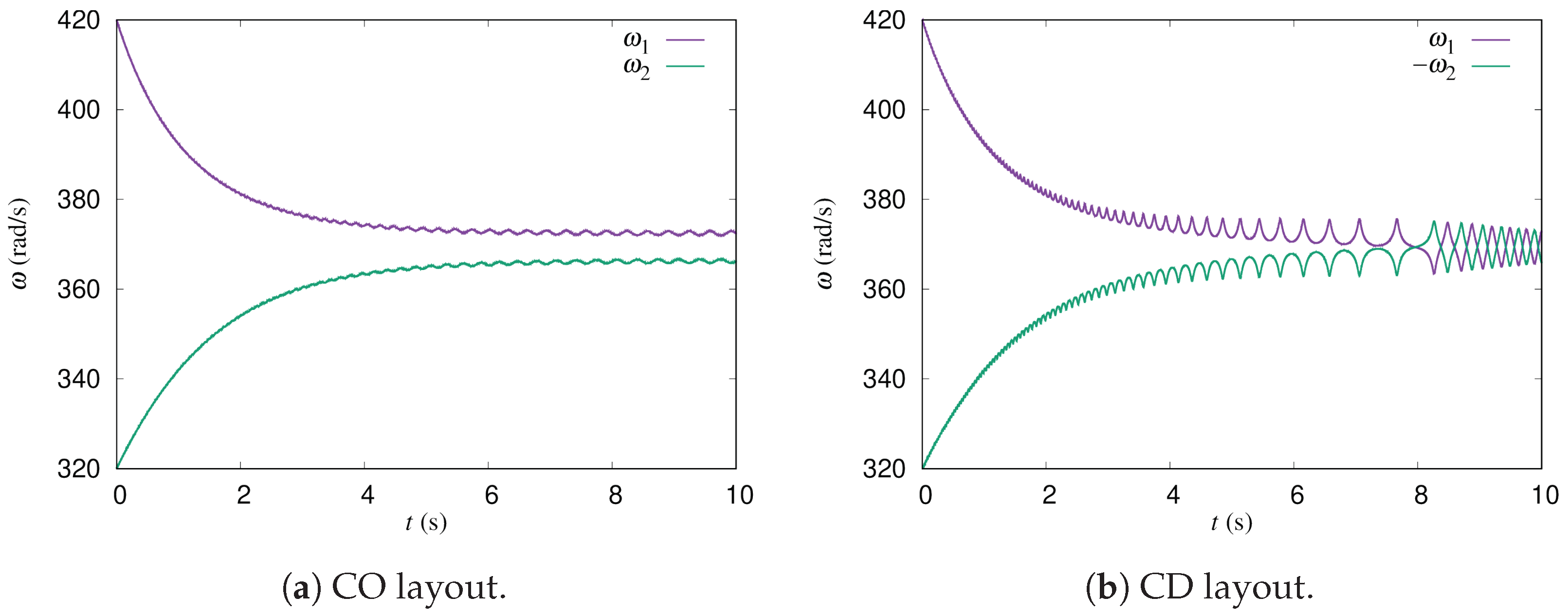
In Refs. [4,5], wind tunnel experiments of a pair of two-bladed H-type Darrieus turbines were reported, and synchronization of the rotations was found in both counter-down (CD) and counter-up (CU) layouts. Note that, in the CD layout, the blades of the two rotors move in the downwind direction in the gap region between the rotors. In the CU layout, the blades move in the upwind direction in the gap region. It was found that the rotational speeds equalize and the power output increases. Let us call this phenomenon phase synchronization. It was also found that the phase difference between the rotors oscillates around a mean value, and converges to it during the phase synchronization period. However, the mechanism of phase synchronization was not discussed in their papers.

Jodai et al. performed wind tunnel experiments on a pair of closely spaced, small-sized rotors made by a 3D printer and found that phase synchronization occurs when the distance between the rotors is sufficiently small in the CD layout [7,8]. It was found that the rotational speed with phase synchronization was 13% greater than that for a single rotor under the extremely small gap condition; the gap distance was 10% of the rotor diameter. This was the first report on the steep rise of the rotational speed under phase synchronization of a pair of closely spaced VAWTs with the extremely small gap. The oscillation of the phase difference was not reported in their papers.

Hara et al. performed a two-dimensional CFD analysis [13,14] to simulate the experiments by Jodai et al. They adopted a dynamic fluid–body interaction (DFBI) model that enabled the angular velocities of the rotors to change dynamically. The simulation results showed that phase synchronization also occurred in the CFD analysis for both the CD and CU layouts. They also found that the angular velocities of the rotors oscillated around the mean value during phase synchronization. Note that the oscillation of the angular velocities around the mean value means the same as the oscillation of the phase difference. From the observations of the CFD simulation results, it was proposed that phase synchronization and the oscillation of the angular velocities occur because of the interaction torques generated by pressure fluctuations in the gap between the rotors. In fact, they found that the velocity increases and the pressure decreases according to Bernoulli’s law when blades of the two rotors come closer together in the gap region.

In this study, we developed an analytical model for the interaction torques that can be included in evolution equations of the angular velocities of rotors considered as solid bodies. Such a model is useful to understand the physics of the observed phenomena. Here, we present the details of the derivation, as well as numerical results showing the phase synchronization and the oscillation of the angular velocities. We also perform a simulation of a pair of rotors with slightly different torque characteristics and show that phase synchronization also occurs if interaction torques exist.

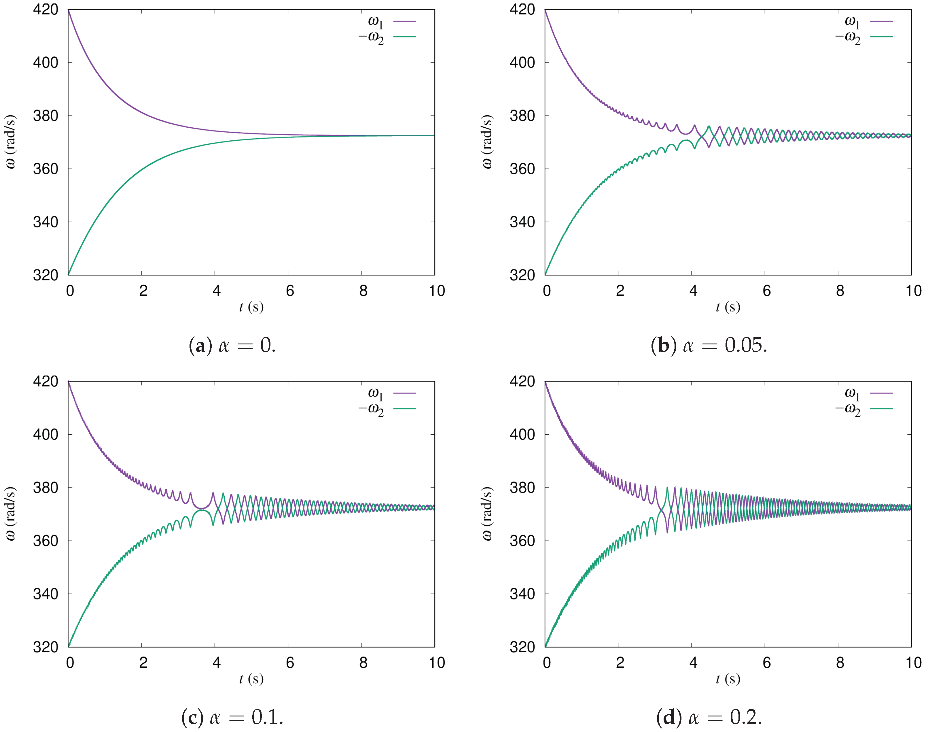
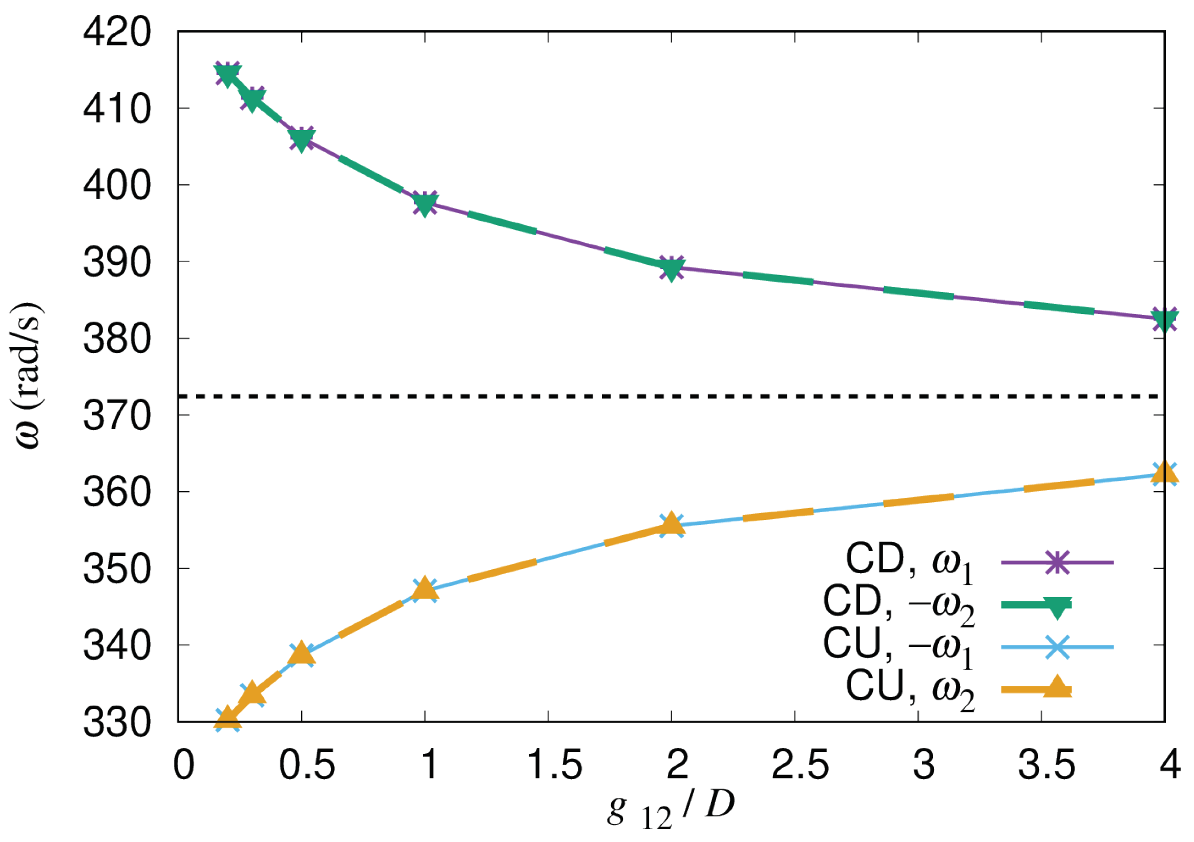
This paper is organized as follows. The details of the model, including the derivation of the interaction torques, are explained in Section 2. Then, Section 3 shows the numerical results based on the model. In particular, in Section 3.2, we report that the phase synchronization and oscillation of the angular velocities occur when using our model. 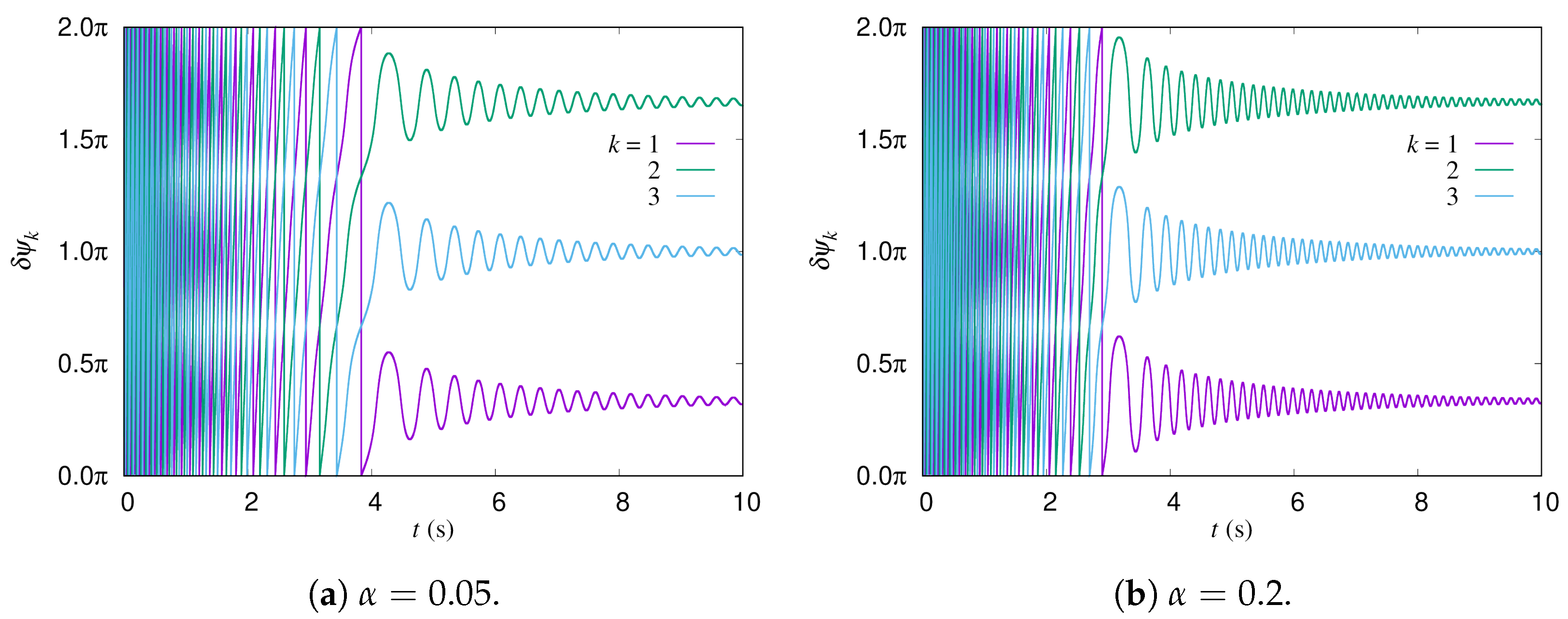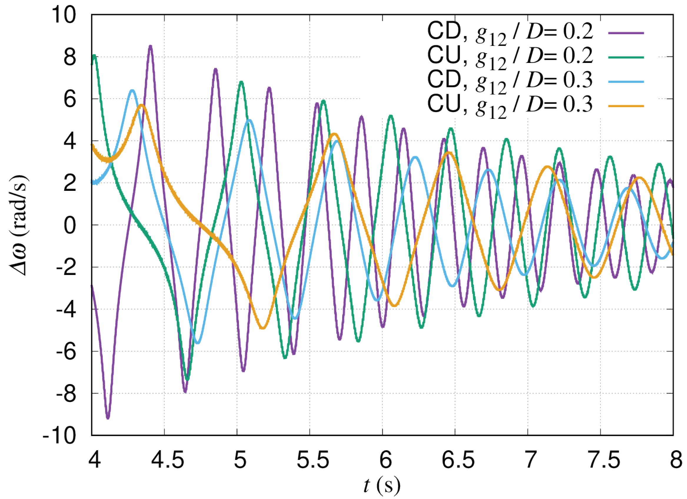We also report the dependence of the angular velocities in the phase synchronization regime on the gap in Section 3.3. The oscillations of the difference in angular velocities are shown in Section 3.4. The conclusions are given in Section 4. 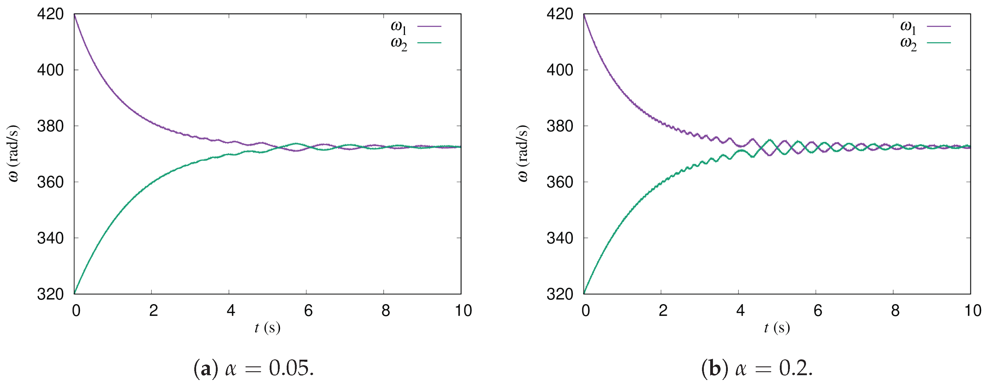Appendix A shows the verification of our model based on comparison with CFD as well as experimental results, while Appendix B summarizes normalized expressions of our model.

2. Model

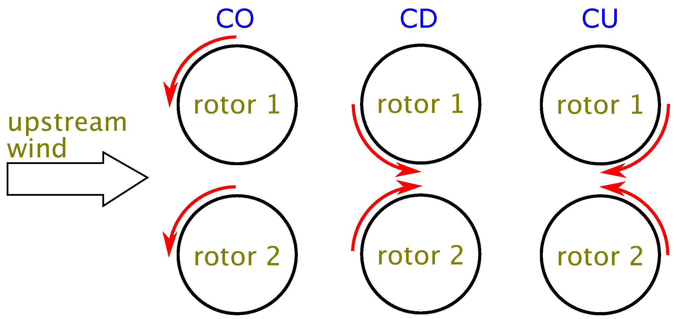
Let us consider a pair of VAWTs. The geometry of the layout is shown in Figure 1. The upstream wind flows from the left of the figure. The rotation directions of the rotors are shown by the arrows. Co-rotating, Counter Down, and Counter Up layouts are written as CO, CD, and CU, respectively. In the CD layout, the blades of the rotors move in the downwind direction in the gap region between the rotors. In contrast, in the CU layout, the blades move in the upwind direction.

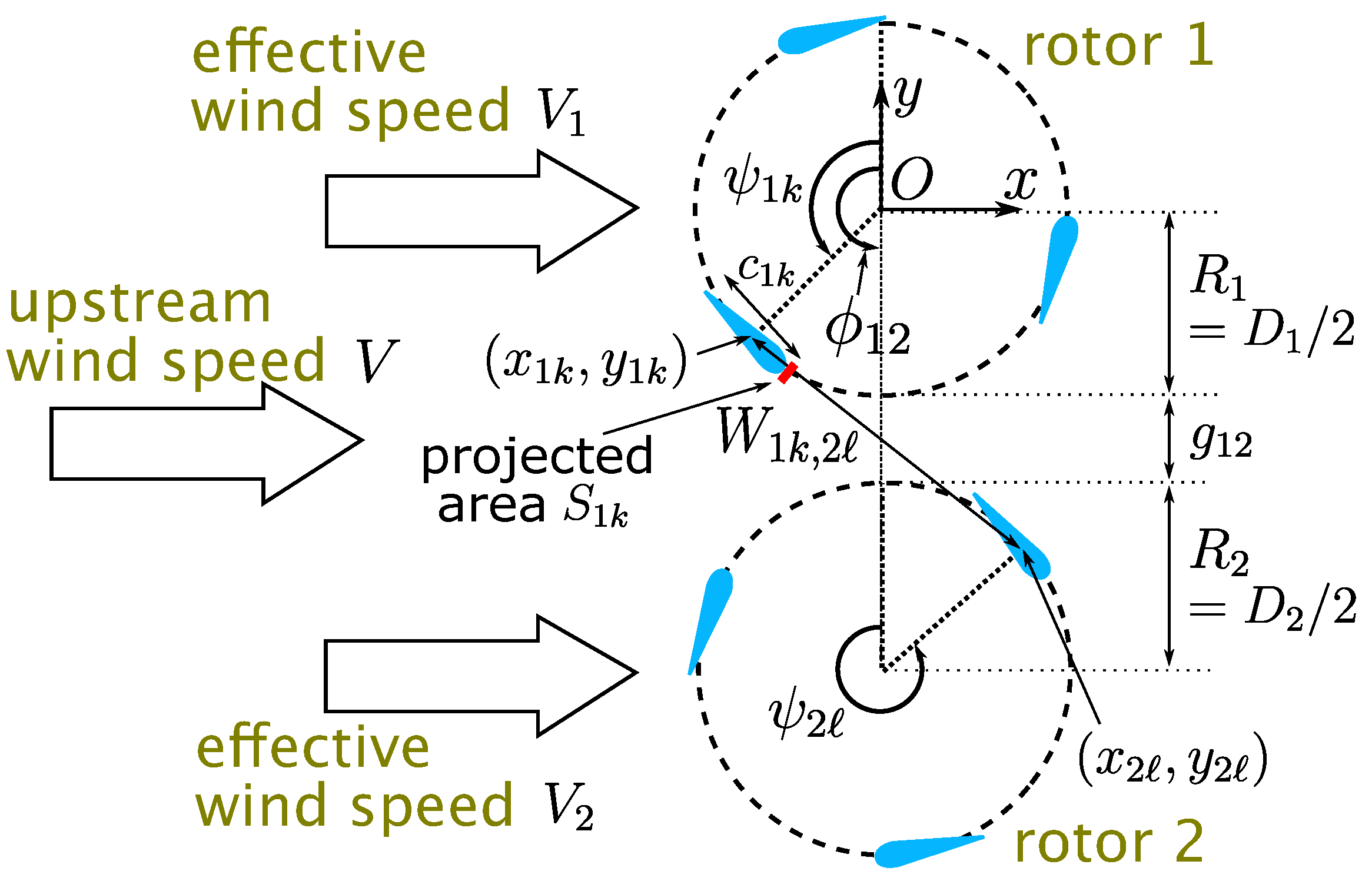
Figure 2 explains the definitions of variables. The diameter and the radius of a rotor i are denoted by $D_i$ and $R_i$, respectively. The gap between rotors i and j is given by $g_{ij}$. In this study, we only considered a pair of rotors. A rotor i has $n_i$ blades, and the position of a blade k is expressed as $(x_{ik},y_{ik})$ in the two-dimensional plane, of which the origin is at the center of rotor 1. An azimuthal angle of a blade k of a rotor i is expressed by ${\psi }_{ik}$, which is zero in the direction of the y axis and increases in the counterclockwise direction. The blades of a rotor are equally spaced in the azimuthal angle, and thus the angle between the neighboring blades is $2\pi /n_i$. The chord length and the area projected along the rotation direction of a blade k of a rotor i are denoted $c_{ik}$ and $S_{ik}$, respectively.

The distance between the blade k of the rotor i and the blade ℓ of the rotor j is written as $W_{ik,j\ell }$, which varies in time due to the rotation. As we explain later in this section, we adopted a model to describe a change in the flow velocity according to the temporal change of $W_{ik,j\ell }$, leading to a pressure fluctuation between the blades according to Bernoulli’s law. The center of the rotor j is in the direction of an angle ${\varphi }_{ij}$ seen from the center of rotor i. As with the azimuthal angle ${\psi }_{ik}$, the angle ${\varphi }_{ij}$ is also zero in the direction of the y axis and increases in the counterclockwise direction. The angle of the center of the rotor i seen from the center of the rotor j is ${\varphi }_{ji}$, although only ${\varphi }_{12}$ with $i=1$ and $j=2$ is shown in Figure 2.

The wind flows in the direction of the x axis. The upstream speed is denoted by V. The flow velocity experienced by the rotor differs for each rotor. The effective flow velocity immediately in front of rotor i is written as $V_i$.

As mentioned above, we only considered a pair of rotors. The evolution equations governing the rotation are

$$\begin{array}{cc}\hfill I_i\frac{\mathrm{d}{\omega }_i}{\mathrm{d}t}& =Q_i-L_i+Q_{\mathrm{p}i},\hfill \end{array}$$

(1)

$$\begin{array}{cc}\hfill \frac{\mathrm{d}{\psi }_i}{\mathrm{d}t}& ={\omega }_i,\hfill \end{array}$$

(2)

where $i=1,2$ represent the two rotors, ${\omega }_i$ is the angular velocity, ${\psi }_i:={\psi }_{i1}$ is the azimuthal angle of a representative blade, $I_i$ is the moment of inertia, $Q_i$ is the rotor torque, $L_i$ is the load torque, and $Q_{\mathrm{p}i}$ is the torque due to the interaction with the other rotor $j(\ne i)$ through pressure fluctuation in the gap between them. Note that ${\psi }_i$ is not necessarily ${\psi }_{i1}$ but can be another ${\psi }_{ik}$ with $k\ne 1$; the meaning is the same for any choice of $k=1,\dots ,n_i$.

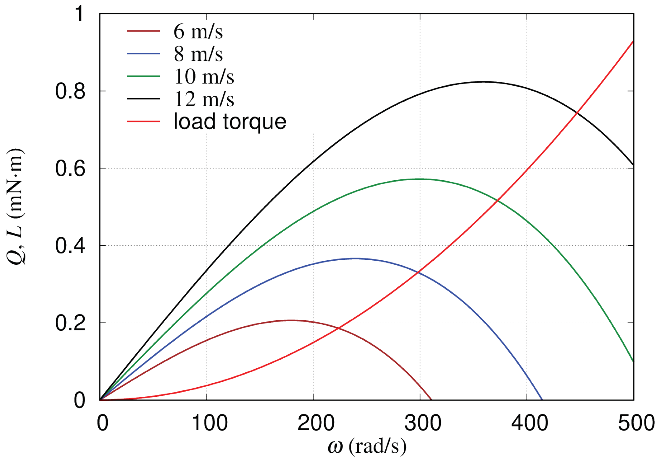
In the following section, we explain our torque models. First, we take the rotor torque $Q_i$ as

$$Q_i=-\frac{3\sqrt{3}{Q}_{\max }\left(V_i\right)}{2{\omega }_0^3\left(V_i\right)}{\omega }_i({\omega }_i+{\omega }_0\left(V_i\right))({\omega }_i-{\omega }_0\left(V_i\right))F_{n_i}\left({\psi }_i\right).$$

(3)

This torque, without the last term $F_{n_i}\left({\psi }_i\right)$, simulates the torque characteristics in the two-dimensional CFD by Hara et al., as shown in Figure 2 of Ref. [14]. Note that the rotor is operated at an angular velocity, in a sense of average over phase, where the torque in Equation (3) is balanced by a load torque introduced below. Since the balanced state occurs at an angular velocity larger than that at the maximum torque in the present choice of the load torque for a given flow velocity, the rotor torque characteristics at small angular velocity regime is not essential. Here, $F_{n_i}\left({\psi }_i\right)$ expresses a modulation in the rotor torque depending on the angle of the blades, which we explain shortly. Without this modulation, or setting $F_{n_i}\left({\psi }_i\right)\equiv 1$, $Q_i$ is a cubic function of ${\omega }_i$ for a given $V_i$ and takes a maximum value $Q_{\max }\left(V_i\right)$ when ${\omega }_i={\omega }_0\left(V_i\right)/\sqrt{3}$ on the positive ${\omega }_i$ side. When ${\omega }_i={\omega }_0$ at the positive ${\omega }_i$ side, the rotor torque becomes zero. Thus, ${\omega }_0$ is sometimes called no-load angular velocity.

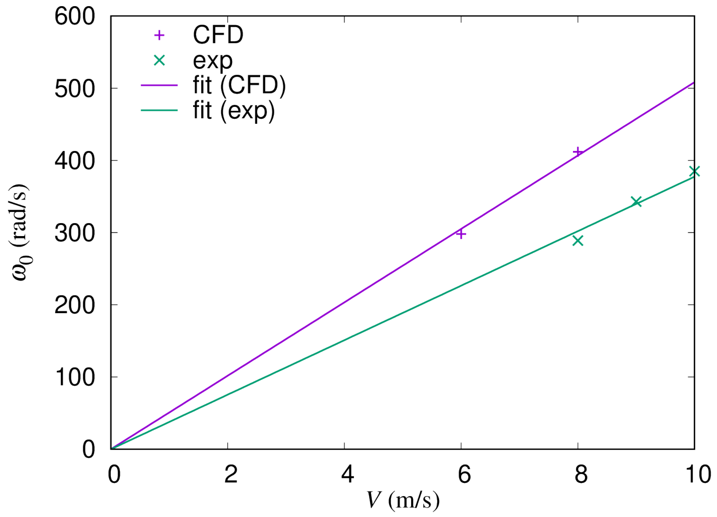
Here, we take

$$\begin{array}{cc}\hfill Q_{\max }\left(V_i\right)& =c_1{V}_i^2,\hfill \end{array}$$

(4)

$$\begin{array}{cc}\hfill {\omega }_0\left(V_i\right)& =c_2{V}_i,\hfill \end{array}$$

(5)

where $c_1$ and $c_2$ are constants. As shown in Appendix A, we chose these expressions by observing the CFD [13,14], as well as the experimental [7,8] data. The actual values used in our simulation are given in the next section. Note that normalized expressions of Equations (3)–(5), as well as equations to appear below are given in Appendix B, where it is shown that the normalized rotor torque $Q_i$ is expressed by a tip–speed ratio ${\lambda }_i:=R_i{\omega }_i/V_i$ for the rotor i and normalized $Q_{\max }$ and ${\omega }_0$ only.

The average of $F_{n_i}\left(\psi \right)$ over $\psi$ is taken to be unity. As shown in Appendix A, it is known that the rotor torque by a single blade is finite at the upstream side and becomes maximal when a blade comes to the position ${\psi }_i=\pi /2$. It decreases to almost zero at the downstream side when the rotor solidity ${\sigma }_i:=n_i{c}_{ik}/\left(\pi D_i\right)$ is large. We assume that

$$F_1\left(\psi \right)=\left\{\begin{array}{cc}4{sin}^2\psi \hfill & (0\le \psi \le \pi )\hfill \\ 0\hfill & (\pi <\psi <2\pi )\hfill \end{array}\right.$$

(6)

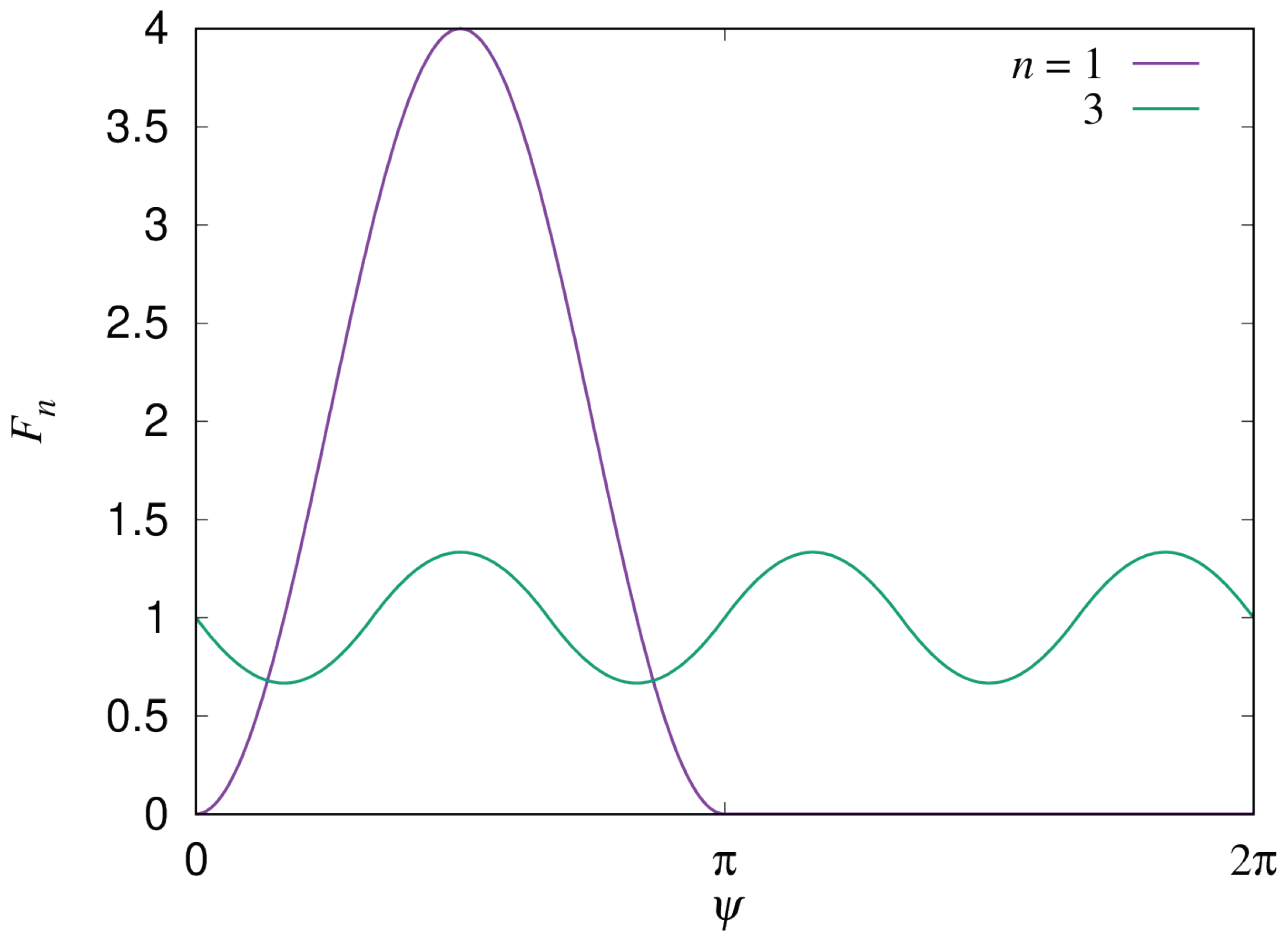
for a single blade. Figure 3 shows the azimuthal angle $\psi$ dependence of $F_n\left(\psi \right)$. In the figure, $n=1$ plots Equation (6). The curve of $n=3$ plots a summation of the modulation function for $n=1$ over three blades equally spaced in the azimuthal angle and normalized such that ${\int }_0^{2\pi }{F}_3\left(\psi \right)\mathrm{d}\psi /\left(2\pi \right)=1$. Note that the function for the modulation can be rather flexibly chosen since it is enough to simulate qualitative aspects of the torque modulation. Any function with its maximum at $\psi =\pi /2$ and almost zero in the downstream half may be acceptable.

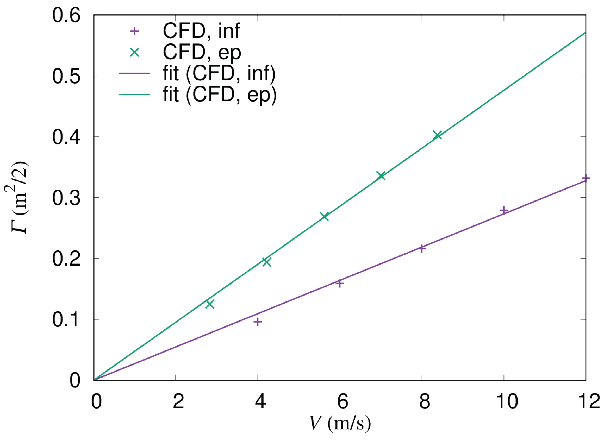
For the effective wind speed, we use

$$V_i=(1-a_i)V+\sum _{j\ne i}\frac{{\Gamma }_j}{2\pi (R_i+R_j+g_{ij})}cos{\varphi }_{ij},$$

(7)

where $a_i$ is a coefficient of self-induced velocity, and ${\Gamma }_j$ is the circulation of rotor j. The second term expresses the velocity induced by another rotor. This assumption, assigning a circulation for a rotor, is similar to the one in Ref. [16]. We take

$${\Gamma }_j=c_3{V}_j,$$

(8)

where $c_3$ is a constant. This dependence was also obtained by the CFD results as shown in Appendix A. By using the effective wind speed $V_i$, the rotor torque on rotor i can be calculated. Note that $V_i$ in Equation (7), especially its mutually induced velocity in the second term of the right-hand side, is evaluated by using the coordinate of the center of rotor i. In reality, the effective flow velocity is different for each blade, and the summation of the torques on every blade of a rotor determines the rotor torque. However, in this study, the effective velocity $V_i$ is used for calculating the rotor torque as an average of the effective velocities for all blades in the rotor, and we assume that $V_i$ is the flow velocity immediately in front of rotor i. Instead of considering the torques on each blade, we take into account the torque modulation of the rotor torque via $F_{n_i}\left(\psi \right)$. The modulation expresses the fact that the blade experiences significantly smaller flow than the upstream when it is in the downstream half of the rotation.

Secondly, we take the load torque as

$$L_i=c_4{\omega }_i^2.$$

(9)

The dependence, square of angular velocity, is known as the ideal load torque to obtain highest power at each instance [17]. The CFD simulations by Hara et al. [13,14] also adopted the ideal load torque of the same form. Within our torque model, it is shown that the load torque in Equation (9) works to keep the highest power as follows. According to the rotor torque in Equation (3), the power $Q_i{\omega }_i$ takes a maximum value when ${\omega }_i={\omega }_0\left(V_i\right)/\sqrt{2}$, and the corresponding rotor torque is $Q_i=3\sqrt{3}{Q}_{\max }\left(V_i\right)/4\sqrt{2}$. By using Equations (4) and (5), these are written such that the maximum power is obtained when ${\omega }_i=c_2{V}_i/\sqrt{2}$ and the corresponding torque is $Q_i=3\sqrt{3}{c}_1{V}_i^2/4\sqrt{2}$. The ideal operation of the turbine is achieved by balancing the rotor torque $Q_i$ by the load torque $L_i$ for whatever $V_i$. This is realized by setting $L_i\propto {\omega }_i^2$, which is obtained by eliminating $V_i$ in Q by using ${\omega }_i=c_2{V}_i/\sqrt{2}$. The coefficient $c_4$ is determined so that the load torque takes 95% of $Q_i$ when the power becomes maximal for a given $V_i$ in Section 3.1.

Finally, we come to the torque caused by pressure fluctuations between the blades. The positions of the blades of rotors 1 and 2 are given by

$$\begin{array}{cc}\hfill x_{1k}& =-R_{1}sin{\psi }_{1k},\hfill \end{array}$$

(10)

$$\begin{array}{cc}\hfill y_{1k}& =R_{1}cos{\psi }_{1k},\hfill \end{array}$$

(11)

$$\begin{array}{cc}\hfill x_{2\ell }& =-R_{2}sin{\psi }_{2\ell },\hfill \end{array}$$

(12)

$$\begin{array}{cc}\hfill y_{2\ell }& =R_{2}cos{\psi }_{2\ell }-(R_1+R_2+g_{12}).\hfill \end{array}$$

(13)

The distance $W_{1k,2\ell }$ between two blades at $(x_{1k},y_{1k})$ and $(x_{2\ell },y_{2\ell })$ is

$$W_{1k,2\ell }=\sqrt{{(x_{1k}-x_{2\ell })}^2+{(y_{1k}-y_{2\ell })}^2}.$$

(14)

Here, we consider the flow to be incompressible and assume that

$$V_{\mathrm{av}}(R_1+R_2+g_{12})=(V_{\mathrm{av}}+\delta V)W_{1k,2\ell },$$

(15)

where $V_{\mathrm{av}}:=(V_1+V_2)/2$ is the average flow velocity, and $\delta V$ expresses the change in the flow velocity between the two blades due to a change in distance between them. Note that the calculation of $\delta V$ may be improved by taking not only the x component of the flow velocity but also the y component, or taking the distance in the y direction between the blades k and ℓ instead of the distance $W_{1k,2\ell }$ itself. Let us leave this refinement as a future issue. We roughly estimate the change of velocity $\delta V$ in this study. Then, we obtain the pressure fluctuation $\delta p$ using Bernoulli’s law

$$\frac{1}{2}\rho V_{\mathrm{av}}^2+p=\frac{1}{2}\rho {(V_{\mathrm{av}}+\delta V)}^2+p+\delta p,$$

(16)

as

$$\delta p=-\frac{1}{2}\rho \left(2V_{\mathrm{av}}\delta V+{\left(\delta V\right)}^2\right).$$

(17)

Here, the air pressure is written as p. Note that we neglected the effects of viscous force and unsteadiness of the flow. We adopted the Bernoulli’s law to explain interactions between the blades due to pressure fluctuation through the increase in the flow velocity in the x direction observed in the CFD results, as shown in Figure 20 of Ref. [14]. The force on a blade due to this pressure fluctuation is calculated by integrating $-\nabla \delta p$ with the blade volume. The necessary force component is that along the rotation direction $-(\partial \delta p/\partial {\psi }_{ik})/R_i$ for the blade k of the rotor i. As an example, for $i=1$, this is calculated as

$$\begin{array}{cc}\hfill \frac{\partial \delta p}{\partial {\psi }_{1k}}& =-\rho (V_{\mathrm{av}}+\delta V)\frac{\partial \delta V}{\partial {\psi }_{1k}}\hfill \\ \hfill & =-\rho \frac{R_1+R_2+g_{12}}{W_{1k,2\ell }}{V}_{\mathrm{av}}\frac{\partial \delta V}{\partial {\psi }_{1k}}.\hfill \end{array}$$

(18)

By using Equation (15),

$$\begin{array}{cc}\hfill \frac{\partial \delta V}{\partial {\psi }_{1k}}& =-\frac{R_1+R_2+g_{12}}{W_{1k,2\ell }^2}{V}_{\mathrm{av}}\frac{\partial W_{1k,2\ell }}{\partial {\psi }_{1k}}\hfill \\ \hfill & =-\frac{R_1+R_2+g_{12}}{W_{1k,2\ell }^3}{V}_{\mathrm{av}}\left[(x_{1k}-x_{2\ell })\right(\frac{\partial x_{1k}}{\partial {\psi }_{1k}}-\frac{\partial x_{2\ell }}{\partial {\psi }_{1k}})\hfill \\ \hfill & +(y_{1k}-y_{2\ell })(\frac{\partial y_{1k}}{\partial {\psi }_{1k}}-\frac{\partial y_{2\ell }}{\partial {\psi }_{1k}})].\hfill \end{array}$$

(19)

Then, we can obtain

$$\begin{array}{cc}\hfill \frac{\partial \delta p}{\partial {\psi }_{1k}}& =\rho V_{\mathrm{av}}^2\frac{{(R_1+R_2+g_{12})}^2}{W_{1k,2\ell }^4}{R}_1\left[R_{2}sin({\psi }_{1k}-{\psi }_{2\ell })\right.\hfill \end{array}$$

$$\begin{array}{cc}\hfill & \left.-(R_1+R_2+g_{12})sin{\psi }_{1k}\right],\hfill \\ \hfill \frac{\partial \delta p}{\partial {\psi }_{2\ell }}& =-\rho V_{\mathrm{av}}^2\frac{{(R_1+R_2+g_{12})}^2}{W_{1k,2\ell }^4}{R}_2\left[R_{1}sin({\psi }_{1k}-{\psi }_{2\ell })\right.\hfill \end{array}$$

(20)

$$\begin{array}{cc}\hfill & \left.-(R_1+R_2+g_{12})sin{\psi }_{2\ell }\right].\hfill \end{array}$$

(21)

The torque on a blade due to pressure fluctuations may be approximated by multiplying the blade volume $c_{ik}{S}_{ik}$ by the rotor radius $R_i$. Now, we also assume that the total torque on a rotor can be obtained by adding contributions from all blades. Then, we obtain

$$\begin{array}{cc}\hfill Q_{\mathrm{p}1}& =-\alpha \sum _{k=1}^{n_i}\sum _{\ell =1}^{n_j}{c}_{1k}{S}_{1k}\rho V_{\mathrm{av}}^2\frac{{(R_1+R_2+g_{12})}^2}{W_{1k,2\ell }^4}{R}_1\left[R_{2}sin({\psi }_{1k}-{\psi }_{2\ell })\right.\hfill \end{array}$$

$$\begin{array}{cc}\hfill & \left.-(R_1+R_2+g_{12})sin{\psi }_{1k}\right],\hfill \\ \hfill Q_{\mathrm{p}2}& =\alpha \sum _{\ell =1}^{n_j}\sum _{k=1}^{n_i}{c}_{2\ell }{S}_{2\ell }\rho V_{\mathrm{av}}^2\frac{{(R_1+R_2+g_{12})}^2}{W_{1k,2\ell }^4}{R}_2\left[R_{1}sin({\psi }_{1k}-{\psi }_{2\ell })\right.\hfill \end{array}$$

(22)

$$\begin{array}{cc}\hfill & \left.-(R_1+R_2+g_{12})sin{\psi }_{2\ell }\right].\hfill \end{array}$$

(23)

Here, a coefficient $\alpha$ is included to control the strength of the interaction between the blades due to the pressure fluctuation, since the summation over all blades may be rather rough. Readers may think that it is strange to add a contribution from a blade at the opposite side of the gap between the rotors; it is natural to count only contributions from blades in the gap region. We also considered a model where rotors are taken as solid cylinders and only considered a narrowed channel between the gap region. This may not be a bad choice for high solidity rotors; however, the flow goes into the region surrounded by the blades of a rotor in reality. Thus, we decided to consider all combinations of blades and to add contributions from all pairs of blades in our model as an average in a sense, although big contributions must arise when two blades come to the gap region, and thus, other contributions may not play major roles. From a numerical computation viewpoint, this assumption, summation over all blades, is far simpler than taking the azimuthal angle of each blade into account to judge whether we should add its contribution or not. The on/off nature of the contributions can yield abrupt changes in torque, leading to a strange time evolution. Thus, we avoid this confusion.

3. Numerical Results

3.1. Characteristics of Rotors

We only consider a pair of rotors and assume that they have completely the same characteristics, except when otherwise stated. The following parameters are chosen. These are the same as those used in the CFD simulations in [13], Hara et al. [14]. The number of blades per rotor is $n_1=n_2=3$. The radius of the rotor is $R_1=R_2=25\mathrm{mm}$. The chord length is $c_{1k}=c_{2\ell }=20\mathrm{mm}$, and the area projected along the rotation direction is $S_{1k}=S_{2\ell }=43.4\mathrm{mm}\times 3.8\mathrm{mm}$ for $k,\ell =1,2,3$. The moment of inertia is $I_1=I_2=5.574\times {10}^{-6}{\mathrm{kg}\mathrm{m}}^2$. Note that the previous CFD simulation [13,14] was two-dimensional, where the rotor height was $1\mathrm{m}$ instead of $43.4\mathrm{mm}$, as used for the three-dimensional model, and the moment of inertia was set at $I_1=I_2=1.284\times {10}^{-4}{\mathrm{kg}\mathrm{m}}^2(=5.574\times {10}^{-6}{\mathrm{kg}\mathrm{m}}^2\times (1\mathrm{m}/43.4\mathrm{mm}))$.

From the CFD simulation for a single rotor with the above parameters, under a fixed angular velocity condition, it was found that the maximum power is obtained when $\omega =366.52\mathrm{rad}/\mathrm{s}$ for $V=10\mathrm{m}/\mathrm{s}$. The time-averaged rotor torque in this case is $Q=0.525\mathrm{mN}·\mathrm{m}$. By using these values, we determined $Q_{\max }\left(V_i\right)$ and ${\omega }_0\left(V_i\right)$ for the rotor torque, Equation (3), and $c_4$ for the load torque, Equation (9). We further determined that $c_1$ and $c_2$ from $Q_{\max }\left(V_i\right)$ and ${\omega }_0\left(V_i\right)$ via Equations (4) and (5).

In the case of our rotor torque (3), the power $Q_i{\omega }_i$ becomes maximal at ${\omega }_i={\omega }_0\left(V_i\right)/\sqrt{2}$ for a given $V_i$. The rotor torque at this angular velocity is $Q_i=3\sqrt{3}{Q}_{\max }\left(V_i\right)/4\sqrt{2}$. We chose this to match the CFD value $Q=0.525\mathrm{mN}·\mathrm{m}$. Therefore, it is assumed that ${\omega }_0\left(10\mathrm{m}/\mathrm{s}\right)=\sqrt{2}\times 366.52\mathrm{rad}/\mathrm{s}$ and $Q_{\max }\left(10\mathrm{m}/\mathrm{s}\right)=(4\sqrt{2}/3\sqrt{3})\times 0.525\mathrm{mN}·\mathrm{m}$. From Equation (4), we determine that

$$\begin{array}{cc}\hfill c_1& =\frac{Q_{\max }\left(V_i\right)}{V_i^2}\hfill \\ \hfill & =\frac{4\sqrt{2}\times 0.525\mathrm{mN}·\mathrm{m}}{3\sqrt{3}\times {\left(10\mathrm{m}/\mathrm{s}\right)}^2}\hfill \\ \hfill & =5.72\times {10}^{-6}\mathrm{kg}.\hfill \end{array}$$

(24)

Additionally, from Equation (5), we obtain

$$\begin{array}{cc}\hfill c_2& =\frac{\sqrt{2}\times 366.52\mathrm{rad}/\mathrm{s}}{10\mathrm{m}/\mathrm{s}}\hfill \\ \hfill & =51.8\frac{\mathrm{rad}}{\mathrm{m}}.\hfill \end{array}$$

(25)

Furthermore, in the CFD simulation, the angular velocity becomes stationary when the load torque is chosen to be 95% of the optimum rotor torque. We assume the same and thus obtain

$$\begin{array}{cc}\hfill c_4& =\frac{L_i}{{\omega }_i^2}\hfill \\ \hfill & =\frac{0.95\times 0.525\mathrm{mN}·\mathrm{m}}{{\left(366.52\mathrm{rad}/\mathrm{s}\right)}^2}\hfill \\ \hfill & =3.71\times {10}^{-9}\frac{\mathrm{kg}·{\mathrm{m}}^2}{{\mathrm{rad}}^2}.\hfill \end{array}$$

(26)

We will set the value of $c_3$ in Section 3.3.

By using these parameters, we obtain the torque curves shown in Figure 4. The rotor torque is plotted for $V=6,8,10$ and $12\mathrm{m}/\mathrm{s}$ without considering the modulation by $F_{n_i}\left(\psi \right)$ and the induced velocities. Note that the rotor torque characteristics at angular velocities lower than the maximum torque for each V are assumed to be different from those of the CFD and the experimental wind turbines to simplify the analysis. The intersection of the rotor torque curve for a given flow velocity and the load torque curve is the a stable steady state. For example, $\omega \simeq 370\mathrm{rad}/\mathrm{s}$ is the angular velocity at the steady state when $V=10\mathrm{m}/\mathrm{s}$. Note that the angular velocity at the steady state for a given flow velocity does not change when the rotor torque Q or $Q_{\max }\left(V\right)$ is multiplied by a constant factor, since the load torque L was chosen to also be multiplied by the same factor in the present study.

Note that the adopted angular velocity values $\omega =366.52\mathrm{rad}/\mathrm{s}$ (3500 rpm) and the torque $Q=0.525\mathrm{mN}·\mathrm{m}$ at the maximum power are slightly different from the values at the steady state ${\omega }_{\mathrm{SI}}=366.1\mathrm{rad}/\mathrm{s}$ (3496 rpm) and $Q_{\mathrm{SI}}=0.485\mathrm{mN}·\mathrm{m}$ obtained in the CFD simulation based on the DFBI for a single rotor [14]. “SI” stands for single. We can use these values of ${\omega }_{\mathrm{SI}}$ and $Q_{\mathrm{SI}}$ instead of those used above to determine $Q_{\max }\left(V\right)$, ${\omega }_0\left(V\right)$ and $c_4$ and then $c_1$ and $c_2$ via Equations (4) and (5) by assuming the following three conditions: (i) the rotor torque balances the load torque at $\omega ={\omega }_{\mathrm{SI}}$, (ii) the balanced torque is $Q=Q_{\mathrm{SI}}$, and (iii) $Q_{\mathrm{SI}}$ is 95% of the torque at the maximum power. We can immediately obtain $Q_{\max }\left(V\right)$ or $c_1$ from the second condition and $c_4$ from the third condition, respectively. We can also obtain ${\omega }_0\left(V\right)$ from the first one, which becomes a cubic equation for ${\omega }_0\left(V\right)$ for a given ${\omega }_{\mathrm{SI}}$. The resulting values are $c_1=5.56\times {10}^{-6}\mathrm{kg}$, $c_2=49.5\mathrm{rad}/\mathrm{m}$, and $c_4=3.62\times {10}^{-9}\mathrm{kg}·{\mathrm{m}}^2/{\mathrm{rad}}^2$, of which relative differences from the values obtained in Equations (24)–(26) and used in the simulations presented in Section 3.2,Section 3.3,Section 3.4 are within 5%. Note that ${\omega }_0\left(V\right)$ was calculated from the cubic equation by a perturbation technique based on a trivial approximate solution ${\omega }_0\left(V\right)/\sqrt{2}\simeq {\omega }_{\mathrm{SI}}$ that gives the maximum power in our model.

3.2. Phase Synchronization

In this Section 3.2, we demonstrate that phase synchronization occurs due to the interaction torque generated by the pressure fluctuation. In order to focus on the effect of the interaction torque, we set $a_i=0$ and $c_3=0$, so that $V_i=V$, i.e., the effective flow velocity is the same as the upstream flow velocity. The upstream velocity used in this section is $V=10\mathrm{m}/\mathrm{s}$. Furthermore, we set $F_{n_i}\left({\psi }_i\right)\equiv 1$ to exclude the effects of torque modulation due to the azimuthal angle of the blade.

We solve the evolution Equations (1) and (2) for $i=1,2$ by the fourth-order Runge–Kutta method. The step size is $(2\pi /n{\omega }_{\mathrm{av}}\left(0\right))/30$, where ${\omega }_{\mathrm{av}}\left(0\right)=\left(\right|{\omega }_1\left(0\right)|+|{\omega }_2\left(0\right)\left|\right)/2$. ${\omega }_{\mathrm{av}}\left(0\right)$ Average of initial angular velocities $\left(\right|{\omega }_1\left(0\right)|+|{\omega }_2\left(0\right)\left|\right)/2$

Figure 5 shows the time evolution of ${\omega }_i$ for $\alpha =0,0.05,0.1$, and $0.2$ in the CD layout. The gap between the rotors is $g_{12}=10\mathrm{mm}$. The initial conditions are ${\omega }_1\left(0\right)=420\mathrm{rad}/\mathrm{s}$, ${\omega }_2\left(0\right)=-320\mathrm{rad}/\mathrm{s}$, ${\psi }_1\left(0\right)=\pi$, and ${\psi }_2\left(0\right)=-0.5$. The initial angular velocities have different magnitudes. One of the blades of rotor 1 is at the narrowest position in the gap initially and that of rotor 2 is slightly ahead.

When $\alpha =0$, the rotors just reach their individual steady states since there is no interaction between the rotors. The rotors have identical characteristics, and thus they rotate at the same angular velocity at the steady state.

When $\alpha$ is finite, the angular velocities oscillate. This simulates the phase synchronization observed in the experiments as well as in the CFD simulations. Such phase synchronization and oscillation of phase difference in the wind tunnel experiments of a pair of two-bladed H-type Darrieus turbines were reported in Section 6.2 of Ref. [4] and in Section 4.4 of Ref. [5]. The phase synchronization and the oscillation of angular velocities in the two-dimensional CFD were reported in Section 3.5 and Figure 17–19, of Ref. [14]. The oscillation period becomes shorter as $\alpha$ increases since the interaction between the rotors becomes stronger. The oscillation period of the angular velocities is about $0.5\mathrm{s}$ for $\alpha =0.05$ at $t\simeq 4\mathrm{s}$, while it is about $0.25\mathrm{s}$ for $\alpha =0.2$. Moreover, the oscillation period becomes shorter over time.

The oscillation amplitude of the angular velocity becomes larger as $\alpha$ is increased. This is also because the interaction becomes stronger as $\alpha$ is increased.

Figure 6 shows the time evolution of the phase differences $\delta {\psi }_k=({\psi }_{11}+{\psi }_{2k})\mathrm{mod}2\pi$ when $\alpha =0.05$ and $\alpha =0.2$. The index k takes a value of $1,2$, or 3. Before the phase synchronization, $\delta {\psi }_k$ runs over the whole range of azimuthal angles. During phase synchronization, on the other hand, $\delta {\psi }_k$ oscillates around a fixed angle. One of the three blades of rotor 2 has a phase difference of $\pi$ with blade 1 of rotor 1, which means that those blades meet in the gap region every rotation. We see that the oscillation period of the angular velocity during phase synchronization is shorter for larger $\alpha$ values, as shown in Figure 6. Moreover, the phase synchronization starts earlier for larger $\alpha$ values.

Phase synchronization occurs also in the CU layout. Since the induced velocity is not taken into account in the simulations presented in this section, the oscillation period and amplitude are the same as those in the CD layout.

Surprisingly, phase synchronization also occurs in the CO layout. The time evolution of $\omega$ for $\alpha =0.05$ and $0.2$ is shown in Figure 7. Compared with the data presented in Figure 5 for the CD layout, the oscillation period of the angular velocities of the CO layout is longer than those of the CD layout with the same $\alpha$ values. We can also see that the oscillation amplitude of the angular velocities is smaller in the CO layout than that in the CD layout. This is of course because the interaction in the CO layout is much weaker than in the CD and CU layouts. In this simulation, the characteristics of the rotors are identical, and thus, the angular velocity is the same at the steady state without the interaction. In the beginning, the magnitudes of ${\omega }_1$ and ${\omega }_2$ are largely different. Thus, they have almost no interaction. However, as the magnitudes of ${\omega }_1$ and ${\omega }_2$ become closer to their steady-state values, the time period that the blades of the rotors stay in the narrow gap region together becomes longer, although it must still be much shorter than that for the CD and CU layouts. This makes the interaction effect visible, even in the CO layout.

In fact, it becomes difficult for phase synchronization to occur if the angular velocities of the rotors at steady state without interaction are different from each other. We set the rotor torque of rotor 2 as 95% of that of rotor 1 while keeping the load torque unchanged. The other parameters are the same as those used in Figure 7. This makes the angular velocity of rotor 2 about $366\mathrm{rad}/\mathrm{s}$ at its steady state without interaction, which is about 1.7% smaller than that of rotor 1. The time evolution of $\omega$ for $\alpha =0.1$ is plotted in Figure 8a. Phase synchronization does not occur in this case. The angular velocities oscillate around each steady-state value. Note that phase synchronization occurs when $\alpha \ge 0.5$, even in this case.

On the other hand, phase synchronization occurs for the CD layout, even at $\alpha =0.1$, which is shown in Figure 8b. The angular velocity of the rotors during phase synchronization is about $369\mathrm{rad}/\mathrm{s}$, which is about an average of the natural values of the two rotors without interaction. Phase synchronization occurs for smaller interactions because the relative speed of the blades of the two rotors is smaller for the CD layout than for the CO layout, leading to a longer interaction duration.

It may be worth pointing out that $\alpha$ can be used to qualitatively reproduce the parameter dependence of the experimental and CFD results on aspects such as the solidity and upstream flow velocity by assuming that $\alpha$ is dependent on these parameters. This is left as a future issue.

3.3. Dependence of the Synchronized Angular Velocity on the Gap

In this Section 3.3, we focus on the dependence of the synchronized angular velocity on the gap, especially when we take into account the mutually induced velocities generated by each component. Therefore, we set $|c_3|=0.0427\mathrm{m}$ according to the CFD simulation results [13,14]. The sign of $c_3$ is positive when $\omega >0$ and negative when $\omega <0$. On the contrary, we set $a_i=0$, since the self-induced velocity by the rotor itself should be the same for identical rotors. When $a_1=a_2$, the effect is only a change in the upstream velocity by a factor of $a_1=a_2$ for both rotors. Note that the torque modulation $F_{n_i}\left({\psi }_i\right)$ in Equation (3) with $n_i=3$ is taken into account in the results presented in this section.

The angular velocity at steady state is plotted against the gap width in Figure 9. Each angular velocity is obtained using the Fourier transform of the time series data at the steady state. We show the results for $\alpha =0.05$, although they are the same for different $\alpha$ values. Additionally, $F_{n_i}\left({\psi }_i\right)$ just introduces modulation of the angular velocity, of which the period is one-third of the rotation period of the rotor and does not affect the phase-synchronized angular velocity.

The magnitudes of the angular velocities ${\omega }_1$ and ${\omega }_2$ agree well in both the CD and CU layouts. The dashed line at $\omega \simeq 372\mathrm{rad}/\mathrm{s}$ is the angular velocity without the mutually induced velocity. The angular velocities at each $g_{12}/D$ are larger (smaller) than this value in the CD (CU) layout. This is due to the induced velocity. The effective velocity is larger (smaller) than the upstream velocity in the CD (CU) layout, as found in the CFD simulation [13,14]. Furthermore, the angular velocity increases (decreases) as the gap is narrowed in the CD (CU) layout because the magnitude of the induced velocity becomes larger for smaller gaps. This dependence can be clearly observed for the CD layout in the experiments [7,8] and the CFD simulations, except for the small gap distances [13,14]. For the CU layout, on the other hand, further analysis is required for comparison with the experiments and the CFD simulations.

3.4. Oscillation Period of the Difference in Angular Velocities

In this Section 3.4, we analyze the oscillation period of the difference of angular velocities $\Delta \omega :=|{\omega }_1|-|{\omega }_2|$. The parameters used are the same as those in Section 3.3. Figure 10 shows the time evolution of $\Delta \omega$ for the CD and CU layouts with $g_{12}/D=0.2$ and $0.3$. The parameter $\alpha =0.05$ was chosen to control the interaction strength for which the oscillation period of $\Delta \omega$ has a comparable order of magnitude with the experiments [4,5] and the CFD simulations [13,14]. The difference $\Delta \omega$ oscillates around 0 during phase synchronization and decays gradually. The oscillation period becomes shorter as time proceeds in all cases, as shown in Figure 10.

First, we found that the oscillation period is longer for the CU layout than the CD layout if the gap distance is the same. For example, the oscillation period is about 0.36 s for the CD layout with $g_{12}/D=0.2$ at around $t=5$ s, while it is about 0.55 s for the CU layout.

Second, we found that the oscillation period is longer for a larger gap distance for a given layout. For example, the oscillation period is about 0.36 s when $g_{12}/D=0.2$ for the CD layout at around $t=5$ s, while it is about 0.62 s when $g_{12}/D=0.3$.

The oscillation period of $\Delta \omega$ seems to be related to the mean angular velocity during phase synchronization; $\Delta \omega$ is longer for smaller mean angular velocities. The mean angular velocity is smaller in the CU layout than in the CD layout because of the mutual induced velocity (see Figure 9). Additionaly, the interaction becomes weaker if the gap distance is larger, thereby the oscillation period becomes longer.

Note that it is difficult to find such trends for the amplitude of $\Delta \omega$, since it decays over time. However, we found that the decay is slower for the CU layout than the CD layout if the gap distance is the same. The damping rate seems to be smaller for longer oscillation periods. The oscillation amplitude for the CD layout with $g_{12}/D=0.2$ is about 7 rad/s at around $t=5$ s. The relative magnitude for the mean angular velocity $\omega \simeq 415$ rad/s is about 1.7%. The relative magnitude is a bit larger for the CU layout, since the mean angular velocity is smaller while the oscillation amplitude is comparable if the gap distance is the same.

4. Conclusions

We developed an analytical model of the interaction torque between two vertical-axis wind turbines through pressure fluctuation. In this model, the pressure fluctuation is obtained according to Bernoulli’s law, taking into account the temporal change in distance between the blades. Although rather crude assumptions were made in the development of the model, our simulations successfully demonstrated the phase synchronization as well as the oscillation of angular velocities around the mean value observed in the experiments and CFD simulations.

Our simulation results show that the angular velocities of the rotors oscillate in time during phase synchronization. When an artificial parameter is changed to strengthen the interaction, the oscillation period becomes shorter and the amplitude becomes larger. This is reasonable physically.

It was also found that phase synchronization occurs even for a pair of rotors with slightly different torque characteristics. This is important because the characteristics of the rotors cannot be identical in experiments.

Our model includes the induced velocities, which change the effective wind speed at each rotor. The simulation results also show that the mutually induced velocity can explain the qualitative dependence of the phase-synchronized angular velocities on the rotational direction of the rotors and the gap distance between them.

The oscillation period of the difference in angular velocities was found to be longer in the CU layout than in the CD layout. Additionally, the oscillation period was found to be longer for larger gap distances. This dependence seems to be related to the mean angular velocity of the rotors during phase synchronization. The mutually induced velocity changed the mean angular velocity in our simulations. The weaker interaction for larger gap distance made the oscillation period longer.