Geothermal Resources Recognition and Characterization on the Basis of Well Logging and Petrophysical Laboratory Data, Polish Case Studies

Abstract

Examples from the Polish clastic and carbonate reservoirs from the Central Polish Anticlinorium, Carpathians and Carpathian Foredeep are presented to illustrate possibilities of using well logging to geothermal resources recognition and characterization. Firstly, there was presented a short description of selected well logs and methodology of determination of petrophysical parameters useful in geothermal investigations: porosity, permeability, fracturing, mineral composition, elasticity of orogeny and mineralization of formation water from well logs. Special attention was allotted to spectral gamma-ray and temperature logs to show their usefulness to radiogenic heat calculation and heat flux modelling. Electric imaging and advanced acoustic logs provided with continuous information on natural and induced fracturing of formation and improved lithology recognition. Wireline and production logging were discussed to present the wealth of methods that could be used. A separate matter was thermal conductivity provided from the laboratory experiments or calculated from the results of the comprehensive interpretation of well logs, i.e., volume or mass of minerals composing the rocks. It was proven that, in geothermal investigations and hydrocarbon prospection, the same petrophysical parameters are considered, and well-logging acquisition equipment and advanced methods of processing and interpretation, developed and improved for almost one hundred years, can be successfully used in the detection and characterization of the potential geothermal reservoirs. It was shown that the newest (current investment)—as well as the old type (archive)—logs provide useful information.

1. Introduction

Sun and gravity determine almost all natural processes that occur on the Earth’s surface. However, only a small part of the solar energy is absorbed and sun heat penetrates a short distance, some tens of centimetres in the case of the daily cycle and a few tens of meters for the annual changes [1]. Temperature, reflecting the volume of heat in the body, influences rock properties and is of great importance in the development and utilization of hydrocarbon and geothermal resources and also mining after the underground gasification of coal. Drying makes the rock cementation weaker which results in porosity increase, while at the same time high temperature causes the thermal increase of grains in the rock, making changes in strength and elastic moduli. Therefore, knowledge on the temperature is important to make the correction and work with real values of physical properties of rocks. Temperature is measured in boreholes, underground mines and on the Earth’s surface, but knowledge on the temperature is only from the nearest part of the Earth’s surface. For many purposes, scientists and engineers construct temperature vs. depth profiles which widely vary with location and geological structure of the site. Laboratory measurements of thermal properties of rocks and mathematical modelling of heat transfer are sources of data for calibration such profiles.

In the textbooks on well logging, diverse borehole thermometers are presented and temperature measurement methods are discussed. However, well logging is the source of extensive data and important information useful in geothermal considerations [2,3,4,5]. Sophisticated well logging methods, dedicated to effective prospection and completion of hydrocarbon deposits, developed for tens of years in the international companies all over the world under high financial outlays and using innovative research facilities and solutions, provide data on porosity, permeability, movable water saturation, irreducible/bound water volume, shaliness, radioactive heat production, temperature and other quantities indispensable in the geothermal resources prospection and characterization. Well logging measurements and interpretation results are also irreplaceable sources of data on lithology, mineral composition, the salinity of formation waters, fracturing in clastic and carbonate reservoirs. In the literature, there are examples of using wireline and production logging for data impossible to be obtained in another way.

The majority of thermal water resources recognized in Poland belong to the low enthalpy ones with a temperature of outflow less or equal to 100 °C. From the beginning, it was known that waters of such temperature can be useful in balneology, recreation and heating [6]. Since the 1960s, in Poland, mostly in the regions well recognized as the hydrocarbon prospection areas some institutions, for instance, Polish Geological Institute appointed to state geological survey, AGH University of Science and Technology, Faculty of Geology Geophysics and Environmental Protection and Faculty of Drilling Oil and Gas, Mineral and Energy Economy Research Institute of the Polish Academy of Sciences and many others started regular, intensive investigations of the geothermal resources [7,8,9,10,11,12,13,14,15,16,17,18,19].

The compact information on the geothermal resources in Poland with an extended list of references is presented in the EOG-Report-GeoHeat-Pol-2017 [20]. In this report, four main hydrogeothermal provinces are characterized: the Polish Lowland, Carpathians, Carpathian Foredeep and the Sudetes. Significant geothermal resources in the Polish Lowland are locally concentrated in the Upper and Middle Jurassic and Lower and Upper Triassic formations [21]. The case of the GT-1 borehole discussed in the paper concerns them. A super-deep borehole in Poland, K-1 (7541 m), in which the highest temperature of the orogeny was measured—178.5 °C [22], was drilled in the Carpathians. The highest temperature of the geothermal water was found in the east part of the Polish Outer Carpathians (BD-1 borehole)—105 °C [7]). In the Western Carpathians, in Poland, the highest temperature was recorded in B IG-1 borehole—127.5 °C [23].

Geothermal waters are the main source of thermal energy. Additionally, hot dry rocks (HDR) can produce heat, first of all in the regions of high volcanic activity but also in the areas of high geothermal gradient. HDR were initially investigated in the Sudetes Mountains, the region of the highest geothermal gradient in Poland, close to the first recognized and utilized thermal waters in balneology [24,25].

Thermal water resource recognition, prospection and production seem to be easier using the highly developed, well equipped and technically recognized methodologies known in hydrocarbon prospection. Historically, geothermal water prospection was joined with table water in hydrogeological investigations. Similar to hydrocarbon reservoirs, water reservoirs are located in clastic and carbonate rocks. So, the methodologies elaborated and still developed for HC prospection can be utilized in geothermal resources investigations, scientific studies and engineering.

2. Theoretical Considerations

2.1. Physical Processes Related to Heat Production and Transport in the Earth

Two main sources of heat are considered in the Earth: a process of slow Earth cooling related to heat transport as conduction and convection/advection and heat generation by the decay of long-lived radioactive isotopes. Conduction is the most significant process of heat transport in the Earth’s crust. Convection becomes important in fluids and gases filling the porous space in rocks and their flow through the permeable formations. The process is not convection but advection, because fluid motion is made by a pressure gradient, not temperature. The average temperature gradient for a geological unit or a selected depth interval multiplied by the mean thermal conductivity of the rocks in the unit/interval enables estimation of heat flux. The temperature gradient can be obtained from the temperature measurements in boreholes, corrected for the environmental influences, to get value at the so-called stable/balanced thermal conditions. It is assumed that the heat flow is only vertical. Heat flow measured in a borehole must be corrected for the effects of local topography and also for influences of the climate changes. Erosion, sedimentation and variability in the thermal conductivity of soils are other factors that may require correction.

The highest concentrations of long-lived radioactive isotopes responsible for the internal heat of the Earth are in the rocks and minerals of the Earth’s crust (

Table 1. Estimates of radioactive heat production in the selected rocks [after 1].

Rock Type/Element	Concentration [ppm/Weight]			Heat Production [10−11 W/kg]
	U	Th	K	U	Th	K	Total
Granite	4.6	18	33	43.8	46.1	11.5	101
Alkali basalt	0.75	2.5	12	7.1	6.4	4.2	18
Continental crust	1.2	4.5	15.5	11.4	11.5	5.4	28
Mantle	0.025	0.087	70	0.238	0.223	0.024	0.49

).

Radioactive isotopes that have a half-life T_1/2 comparable to the age of the Earth are: ²³⁸U, ²³⁵U, ²³²Th and ⁴⁰K (T_1/2 = 4.5 × 10⁹ yr., 7.1 × 10⁸, 1.4 × 10¹⁰ and 1.3 × 10⁹, respectively). They are responsible for radiogenic heat production. The abundance of the radioactive isotope ⁴⁰K in natural potassium is only 0.01167 %, but potassium is a very common element and its heat production plays an important role. The heat amount generated per second by uranium, thorium and potassium is as follows 95.2, 25.6, 0.00348 [μW/kg]. The heat, Qr produced by rock with the C_U, C_Th and C_K concentrations is calculated using formula (1) [26,27] on the basis of laboratory measurements of natural radioactivity.

Qr = 95.2 C_u + 25.6 C_Th + 0.0348 C_k

(1)

The volume concentration of radioactive elements and bulk density from well logs also enable radiogenic heat calculation according to formula (2) [28]:

A = (ρ (9.52 URAN + 2.56 THOR + 3.48 POTA)) × 10⁻⁵

(2)

where: A [μW/m³]—radiogenic heat, ρ [kg/m³]—bulk density, URAN [ppm], THOR [ppm], POTA [%]—uranium, thorium and potassium volumetric contents, respectively.

2.2. Logs That Could Be Used in Geothermal Resources Recognition and Characterization

Gamma-ray (GR) is a simple log measuring the natural radioactivity of rocks, most popular and willingly used by geologists in the primary recognition of lithology. It is a passive method in the group of nuclear logs, fully safe from the environmental protection and human safety viewpoint. GR logging result as one curve—intensity of natural radioactivity vs. depth provides information about the presence of radioactive elements in rocks. GR curve in the potassium mud boreholes should be corrected due to the ⁴⁰K radiation of the borehole fluid. GR is always included in the set of logs used for the comprehensive interpretation, because it provides indispensable information on shaliness, i.e., clay mineral content. In the spectral gamma log, spectral gamma-rays (SGR) are gathered in three energetically separated windows formed around the energy of gamma rays emitted by potassium (1.46 MeV), uranium (1.67 MeV) and thorium (2.62 MeV). SGR acquisition result comprises five quantities: total natural gamma radioactivity, GG [API], natural gamma radioactivity from potassium and thorium, GRS [API], volumetric potassium, POTA [%], uranium, URAN [ppm] and thorium, THOR [ppm] contents. Ratios: Th/K, Th/U, U/K also result from measurements. SGR is also used for shaliness determination but the most important application is clay mineral identification and radioactive heat calculation. Ratios (Th/U and U/K) are used as indicators of fractures, especially in carbonate reservoirs, in which chemical compounds of uranium and even uranium from hydrothermal solutions can crystallize.

Gamma–gamma log, named Density log or spectral gamma–gamma log, named Litho-Density log, belonging to the active nuclear logs group, provides bulk density, RHOB, and photoelectric absorption index, PE. RHOB (bulk density) and DRHO (correction) curves are obtained from both logs. DRHO curve plays an only informative role, together with the caliper, CAL (borehole diameter) log. Due to the special construction of the gamma–gamma devices pushed to the borehole wall, high-value DRHO in the depth section of the increased caliper (cavern) means low credibility of the bulk density. Bulk density belongs to the group of three basic parameters/logs used to calculate total porosity: Density, Neutron and Sonic logs. Total porosity determined from three porosity logs: DPHI, NPHI and SPHI presented in the specific limestone units are compared (overlay) in quick, qualitative interpretation in the lithology characterization.

Neutron logging result, presented as neutron porosity, NPHI, is attributed to the limestone lithology. This quantity reflects the hydrogen content in the formation. In reservoirs, hydrogen is considered in water and hydrocarbons in pore space, in clay minerals, as water bound in the interlayer space and hydroxyl groups. Hydrogen is also present in crystal water, for instance, in gypsum.

The nuclear magnetic resonance log, NMR, one of the modern borehole measurements and laboratory experiments, provides the most important information about the porosity and bound water in the formation, also with pore size and permeability [29,30]. Hydrogen and its location in rock formation play here a crucial role, similar to the Neutron log, but the NMR device, in contrast to Neutron, is free from the radioactive source. In borehole and laboratory measurements based on the NMR phenomenon times of the relaxation of the hydrogen nuclei are considered. The newest NMR laboratory equipment and borehole devices enable differentiating between moveable and bound water (capillary and clay), providing dynamic porosity from measurements of the T1 and T2 relaxation times. NMR porosity is independent of the matrix minerals’ influence.

Shortly characterizing acoustic/sonic logs is worth mentioning that even from the oldest records, i.e., transit interval time (slowness) of elastic P-wave, DT total porosity could be calculated. The physical basis of this log is the changeability of elastic properties of rocks, related to the different mineral composition of the matrix, volume and type of porosity and type of media filling pore space. Nowadays, sophisticated sonic devices, equipped with dipole sources, provide the interpreter with a wealth of elastic parameters enabling total porosity determination, dynamic elastic moduli calculation, synthetic seismogram construction, information on fracturing and orogeny zone of weakness.

Resistivity logs of great variety (classic—normal and lateral, laterologs, induction logs) are used from the very beginning of the hydrocarbon prospecting history to determine water/HC saturation. In the case of geothermal resource recognition and characterization, resistivity can be used to calculate the effective porosity. The oldest Archie formula [3] is frequently used for the effective porosity calculation of the carbonate reservoirs, treated as clean (shaliness free) rocks. Resistivity logs are extremely useful in the comprehensive interpretation, because they are run in all boreholes, in each depth section.

Electric imaging is a relatively novel measurement, relying on the resistivity scanning of the borehole wall. Now, technologically advanced devices operate in boreholes filled with conductive and oil-based muds. Natural and induced fracturing is the most important outcome from this log, apart from the structural dips and azimuths and borehole breakouts. In a similar role, acoustic imaging can be used, but only in the wells filled with muds of relatively low density.

SP log—spontaneous potential recording along the borehole axis belongs to the same group of the simplest and oldest measurements as resistivity, GR and caliper logs. It is a passive log that records the natural liquid-junction potentials generated in the vicinity of the borehole due to the difference in the salinity of mud filtrate and formation water mixing in the invaded zone. It is useful in delineating reservoir formations and in the determination of the resistivity/salinity of formation water.

The special type of logs, important in geothermal investigations are borehole temperature measurements. Here, there is important to define the transient and stable/balanced state of temperature in the borehole and its vicinity. Because drilling fluids (mud, water) circulating in the borehole during the drilling process have a temperature different from the orogeny, the measured temperature of the borehole fluid is not the same as the rock formation. Time (several days or even months, depending on geological conditions) is needed to level up the temperature in the borehole and surrounding rock formation. The frequently met state when the temperature in the borehole differs from the temperature of the surrounding rock is named thermal quasi-equilibrium [31], unlike real equilibrium. Three basic types of temperature measurements in boreholes are considered. Nowadays, the most popular and made in all log runs is bottom hole temperature measurement (BHT) providing an actual temperature (of the borehole fluid) at the bottom of drilled and logged depth section, in the conditions of disturbed thermal equilibrium. Because drilling and logging are realized in sections the outcome of BHT comprises several values, which can be the basis for constructing the temperature log. There are also direct measurements of the transient temperature along the borehole axis in depth sections—thermal logs. They provide the current temperature necessary to make temperature corrections for other logs but also carry information on the orogeny temperature. The so-called stable/balanced temperature logs made in thermal equilibrium are used for thermal gradient determination. They are very important from the geological point of view and provide thermal data close to the real one, but are expensive and rather rare.

2.3. Petrophysical Parameters from Well Logging

The most important parameter is the porosity. Quantity considered as porosity determined from different logs is not the same. Total porosity, PHI can be calculated from individual logs: Density, Neutron and Sonic and also from the comprehensive interpretation of the set of logs. Two symmetric formulas are used for the total porosity calculation from the Density (3) and Sonic (4) logs:

$${\varnothing }_{\mathrm{t}} = \mathrm{PHI} = \frac{{\mathsf{\rho }}_{\mathrm{m}}-\mathsf{\rho }}{{\mathsf{\rho }}_{\mathrm{m}}-{\mathsf{\rho }}_{\mathrm{f}}}$$

(3)

$${\varnothing }_{\mathrm{t}} = \mathrm{PHI} = \frac{\mathrm{DT}-{\mathrm{DT}}_{\mathrm{m}}}{{\mathrm{DT}}_{\mathrm{f}}-{\mathrm{DT}}_{\mathrm{m}}}$$

(4)

where: ${\varnothing }_{\mathrm{t}}$, PHI—total porosity, $\mathsf{\rho }$—logged bulk density (RHOB), ${\mathsf{\rho }}_{\mathrm{m}}$ and ${\mathsf{\rho }}_{\mathrm{f}}$—density of matrix and pore fluid, respectively, DT—logged transit interval time (slowness), ${\mathrm{DT}}_{\mathrm{m}}$ and ${\mathrm{DT}}_{\mathrm{f}}$—transit interval time (slowness) of matrix and pore fluid, respectively.

Calculated total porosity, ${\varnothing }_{\mathrm{t}}$, PHI should be corrected for the shaliness influence, which is very important in clastic rocks. Clays in rock formation cause an increase of the calculated total porosity according to formulas (3 and 4), because recorded RHOB is lowered and recorded DT is enlarged by the shaliness. Total porosity from Equations (3) and (4) is influenced by matrix mineral composition. The interpreter is responsible for the adoption of proper matrix density and slowness, which is relatively easy in carbonates, for instance in dolomites, but is very difficult in sandstones or mudstones. In the case of the latter, weighted average values of the matrix parameters can be calculated, but to do it, volume or mass of minerals building the rock formation should be determined. The comprehensive interpretation, i.e., solution the set of equations, where each equation relates to the individual log provides with the volumes of given matrix minerals and porosity. To obtain total porosity PHI from the neutron porosity, NPHI in clastic rocks shaliness is necessary. The relationship between NPHI and PHI is described by formula (5):

$$\mathrm{NPHI}=\mathrm{PHI}+\mathrm{VSH}\times { \mathrm{NPHI}}_{\mathrm{SH}}$$

(5)

where: NPHI—neutron porosity, VSH—shaliness (volume of clay minerals), NPHI_SH—neutron porosity of shale.

In well logging and core analysis, shale and clay are differentiated in the way, that shale means clayey rock without specifying clay minerals, including other components, for instance, quartz or calcite in pelitic fraction and clay means clay minerals. NPHI_SH changes in a large range depending on the type of dominating clay mineral, from 0.20 for kaolinite to 0.55 for montmorillonite. Comparing various types of porosity which are considered in petrophysical interpretations and delivered by well logging the following inequality (6) can be written:

$$\mathrm{NPHI}\ge \mathrm{PHI}\ge \mathrm{PHIE}\ge {\mathrm{PHI}}_{\mathrm{dyn}}$$

(6)

where NPHI, PHI, PHIE and ${\mathrm{PHI}}_{\mathrm{dyn}}$ are neutron, total, effective and dynamic porosities, respectively. Generally, effective porosity, ${\varnothing }_{\mathrm{ef}}$, PHIE is a result of total porosity, PHI correction for the shaliness. Using resistivity logs and Archie formula [2] (7) effective porosity of clean, i.e., shaliness free rocks can be calculated.

$${\varnothing }_{\mathrm{ef}}={({\mathrm{R}}_{\mathrm{w}}/{\mathrm{R}}_{\mathrm{o}})}^{1/\mathrm{m}}$$

(7)

where: ${\mathrm{R}}_{\mathrm{o}}$ and ${\mathrm{R}}_{\mathrm{w}}$ are resistivities of rock fully saturated with water and resistivity of the water, respectively, m—cementation exponent, equal to 2 in the original Archie formula, but needed to be defined in individual interpretation of clastic rocks (1.3 < m < 2).

Effective porosity value reflects pore space open for electric current flow. It comprises water bound in capillary and clay minerals. The difference between effective and dynamic porosity is related to the difference in the physical basis of resistivity and NMR logs. NMR provides dynamic porosity, ${\mathrm{PHI}}_{\mathrm{dyn}}$, which comprises only moveable part of pore water.

Shaliness or volume of clay minerals, $\mathrm{VSH}$ can be obtained from GR or SGR logs and calculated from the comprehensive interpretation of the set of logs. The frequently used empirical Larionov formulas [3] (8–10) for $\mathrm{VSH}$ calculation are presented as follows:

$$\mathrm{VSH}=0.33\times \left(2^{2{\mathrm{I}}_{\mathrm{GR}}}-1\right)$$

(8)

$$\mathrm{VSH}=0.083\times \left(2^{3.7{\mathrm{I}}_{\mathrm{GR}}}-1\right)$$

(9)

$${\mathrm{I}}_{\mathrm{GR}}=\frac{\mathrm{GR}-{\mathrm{GR}}_{\min }}{{\mathrm{GR}}_{\max }-{\mathrm{GR}}_{\min }}$$

(10)

where: $\mathrm{VSH}$—shaliness (volume of clay minerals), ${\mathrm{I}}_{\mathrm{GR}}$—gamma-ray index, $\mathrm{GR}$—current GR value, ${\mathrm{GR}}_{\min }$ and ${\mathrm{GR}}_{\max }$—minimal and maximal values of GR curve in the interpreted formation, respectively. Formula (8) is dedicated for the older than Tertiary, consolidated rocks, (9)—for the Tertiary, unconsolidated rocks.

SP curves (Spontaneous Potential log) in formations drilled with old type muds being the suspension of clays in water provide credible information on resistivity, next salinity of formation water [2]. Additionally, sophisticated nomograms can be used to recognize the type of salts composing formation water, which is highly important in geothermal considerations.

$${\mathrm{E}}_{\mathrm{SP}}={\mathrm{K}}_{\mathrm{SP}}\times \log \frac{{\mathrm{R}}_{\mathrm{mfe}}}{{\mathrm{R}}_{\mathrm{we}}}$$

(11)

where: ${\mathrm{E}}_{\mathrm{SP}}$—SP anomaly read in thick, clean porous, permeable bed, ${\mathrm{K}}_{\mathrm{SP}}$—liquid junction coefficient, ${\mathrm{R}}_{\mathrm{mfe}}$ and ${\mathrm{R}}_{\mathrm{we}}$—equivalent resistivity of mud filtrate and formation water, respectively.

Petrophysical parameters and other quantities interpreted from borehole curves were shortly presented to point out the importance and usefulness of well logging in geothermal investigations. Advantage means continuous data collected in situ, also a great variety of logs based on different physical phenomena, delivering data complementary to each other, not redundant. Disadvantage means data gathered along the borehole axis and necessity to extrapolate it into 3D volume considered in seismic using, for instance, geostatistical methods because borehole sites are irregular and their density is rather low. Formulas presented in the paper are used in the commercial computer systems for interpretation of well logs and integrating data from various geological and geophysical sources. The authors would like to share the basic knowledge and explicitly present the equations to enable understanding the selection of options available in systems.

2.4. Thermal Conductivity Laboratory Measurements

There are many results of laboratory thermal conductivity, λ measurements of minerals and rocks (e.g., [32]) and also many published solutions on thermal conductivity calculated on the basis of mineral composition or porosity–lithology interpretation of the set of well logs [33]). Heat flow to the surface strongly depends on the thermal conductivity of rocks in the Earth’s crust and mantle, and recognition of it in the region is important from an ecological point of view, considering geothermal heat pumps as sources of energy [34,35]. Thermal conductivity is closely related to other petrophysical parameters and similarly to electric and elastic properties depends on mineral composition, material density, grain size and porosity. Pore space saturation, i.e., volume and type of medium in rock formation also influences thermal conductivity—the lowest values are characteristic for gas saturated rocks. The λ parameter can show large variations in the results of laboratory measurements and calculations, so the harmonic mean of results from some samples is recommended. A short description of laboratory equipment is presented on the basis of the set available at the Petrophysical Laboratory at the Faculty of Geology Geophysics and Environmental Protection, AGH UST, Krakow, Poland, consisting of FOX 50 Heat Flow Meter, TA Instruments with pump and recirculating chiller automatically managed by computer [36]. Rock samples of the diameter 0.05–0.062 m and the maximum thickness equal to 0.025 m (~1 inch) should have two parallel surfaces and be polished up to ensure the measurement accuracy. Temperature range covers 10—110 °C with resolution: ±0.01 °C.

3. Results

The examples given are from the reservoir formations drilled by boreholes (GT-1, GT-2, K-1, S-1 and L-4) in the Polish territory, in different geological units (Figure 1). GT-1 (2925.5 m) and GT-2 (2361 m) boreholes were drilled (2008–2009 years) to recognize the geothermal potential of the Mesozoic formations in the Central Polish Anticlinorium (

Table 2. Stratigraphy and lithology of the formations drilled by GT-1 and GT-2 boreholes (on the basis of the report entitled “Opracowanie wyników pomiarów geofizycznych w otworze GT-1, Geofizyka Toruń S.A., 2008”).

GT-1		Both Boreholes—GT-1 and GT-2		GT-2
Depth Interval [m]	Lithology	Stratigraphy	Stratigraphy Code	Lithology	Depth Interval [m]
0.0–76.0	Sand, clay, sandy clay, loam, brown coal	Quaternary + Neogene + Paleogene	Q + Ng + Pg	Sand, clay, sandy clay, loam, brown coal	0.0–59.0
76.0–195.5	Marly limestones, marls, marly claystones, claystones	Upper Cretaceous	K3	Marly limestones, marls, marly claystones, claystones	59–142
195.5–541.0	Sandstones, claystones, limestone inserts	Lower Cretaceous	K1	Claystones, marly claystones, shaly sandstones,	142–553
541–1267	Gypsum, marls, limestones, marlyclaystones	Upper Jurassic	J3	Gypsum, marls, marly limestones, limestones	553–1279.5
1267–1776.5	Alternate packets of sandstones, shaly sandstones, claystones	Middle Jurassic	J2	Alternate packets of sandstones, shaly sandstones, claystones	1279.5–1792.5
1776.5–1820	Sandstones with admixture of calcareous substance	Lower Jurassic	J1; Borucice Beds	Sandstones with admixture of calcareous substance	1792.5–1829
1820–1905	Mudstones and claystones with calcareous substance	Lower Jurassic	J1; Ciechocinek Beds	Mudstones and claystones with calcareous substance	1829–1936.5
1905–1971	Sandstones with mudstone and claystone intercalations	Lower Jurassic	J1; Upper Sławęcice Beds	Sandstones with mudstone and claystone intercalations	1936.5–1973.5
1971–2132	Sandstone, mudstone, claystone	Lower Jurassic	J1; Main Sławęcice Beds	Sandstones separated with mudstone and claystone	1973.5–2136
2132–2335.5	Thick-layered sandstones	Lower Jurassic	J1; Ksawerów and Kłodawa Beds	Thick-layered sandstones, locally separated with claystones and mudstones	2136–2349
2335.5–2528	Sandstones intercalated by mudstones and claystones	Upper Triassic	TRe; Rhaetian	Clayey and muddy formation with sandstones	2349–2362 *
2528–2755	Clayey and muddy formations with calcareous and dolomitic substance	Upper Triassic	TK; Keuper
2755–2883.5	Carbonate–anhydrite formations: dolomites, anhydrite, marls	Middle Triassic	T2; Muschelkalk
2883.5–2925 *	Marly claystones, marls, marly and dolomitic limestones	Lower Triassic	Tp3; BunterSandstone (Ret)

*—end of well (TD).

). The temperature measurements from the very deep K-1 borehole (7541 m), drilled over several years in the Carpathians, were the examples of temperature logging made in the temperature balanced conditions for the geothermal gradient determination. The SGR log from S-1 borehole, also from the Carpathians, enabled radiogenic heat calculations to compare the results with those obtained in GT-1, to underline the relationship between lithology and stratigraphy, thermal conductivity and volume of generated heat flux. The last example, from L-4 borehole in the Carpathian Foredeep, showed how the modern NMR log could bring extended information on porosity. In the boreholes, various sets of well logs and results of the comprehensive interpretation together with the outcomes of laboratory measurements were used to determine petrophysical parameters useful in geothermal resource characterization.

Lithological and stratigraphic information presented in detail in Table 2 informs about the sequence of formations forming the orogeny, which could be recognized using well-logging measurement and interpretation results, next used for proper adopting/calculation of thermal conductivity for temperature and heat flux modelling.

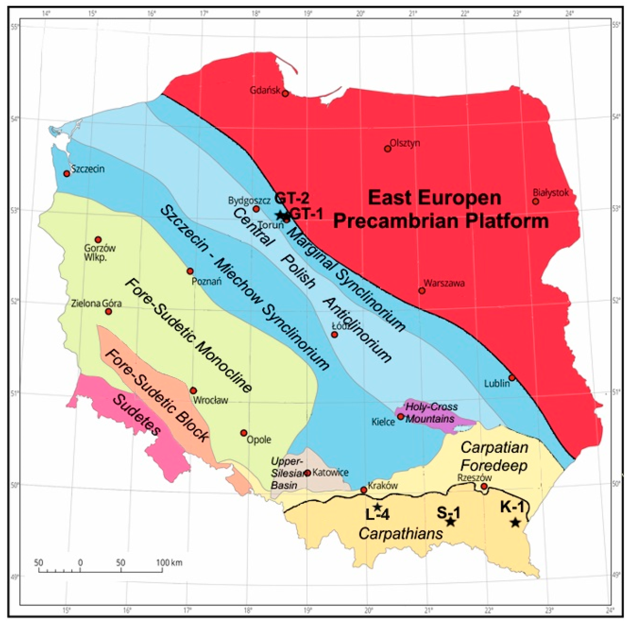
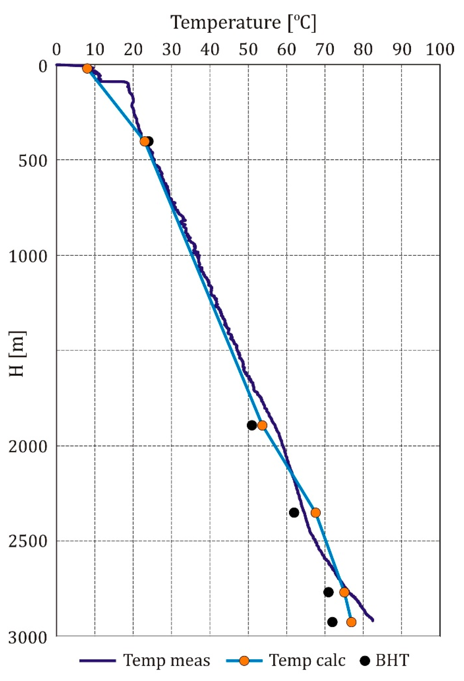
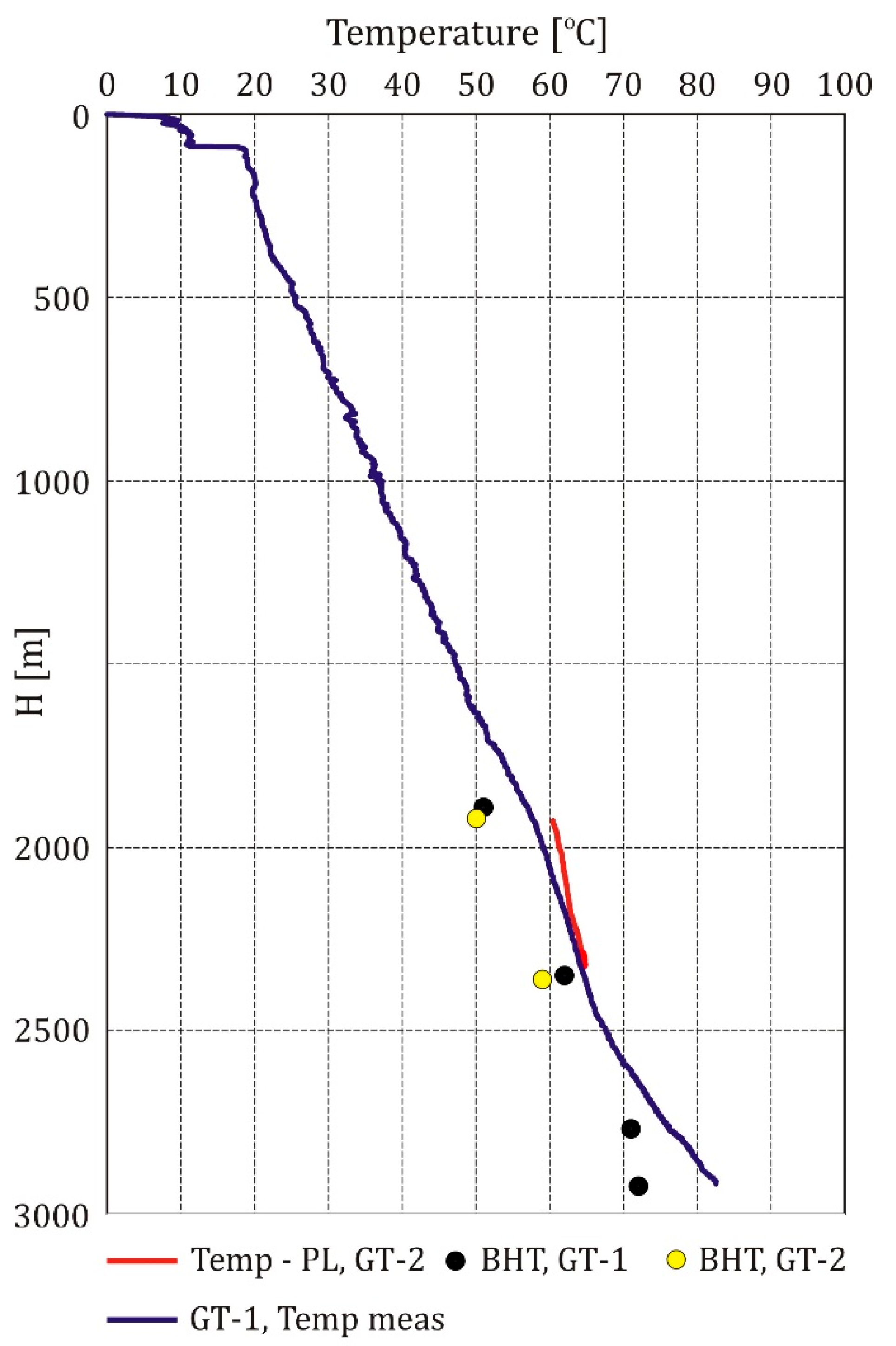
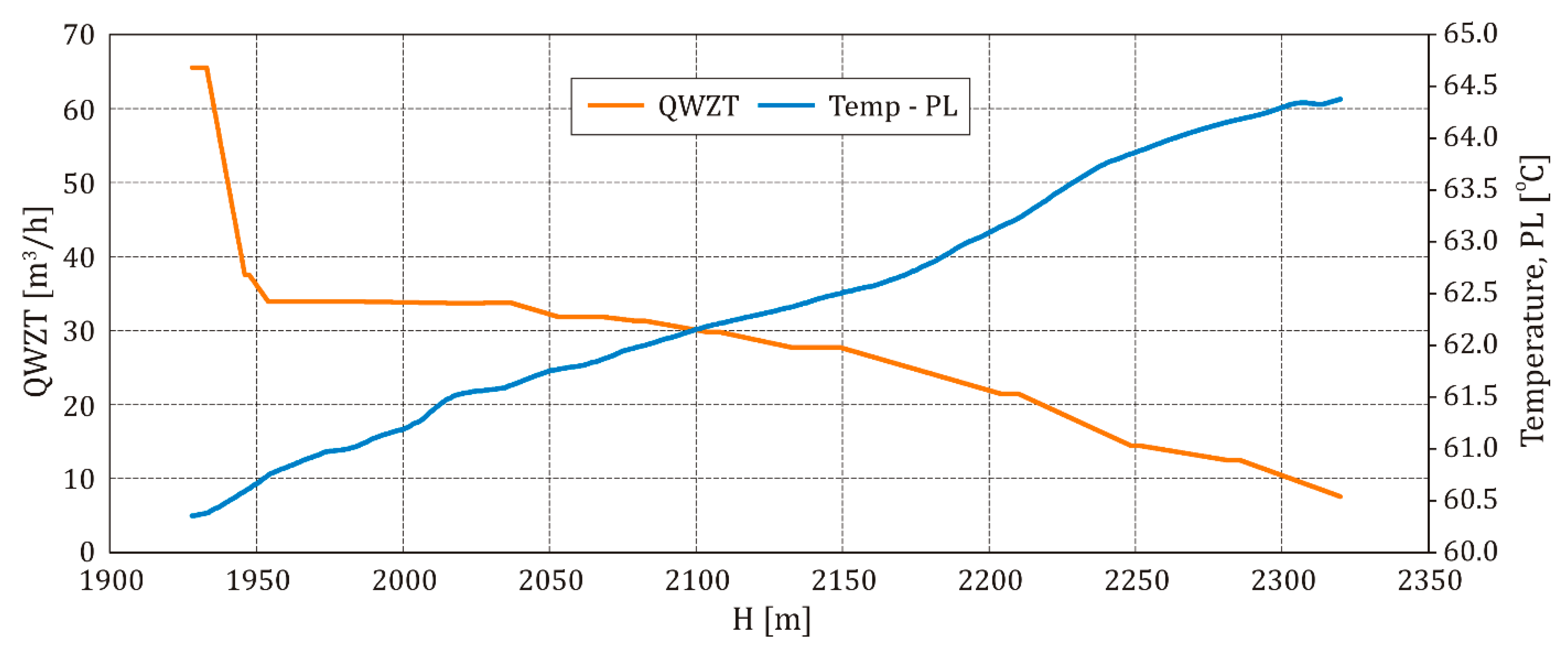
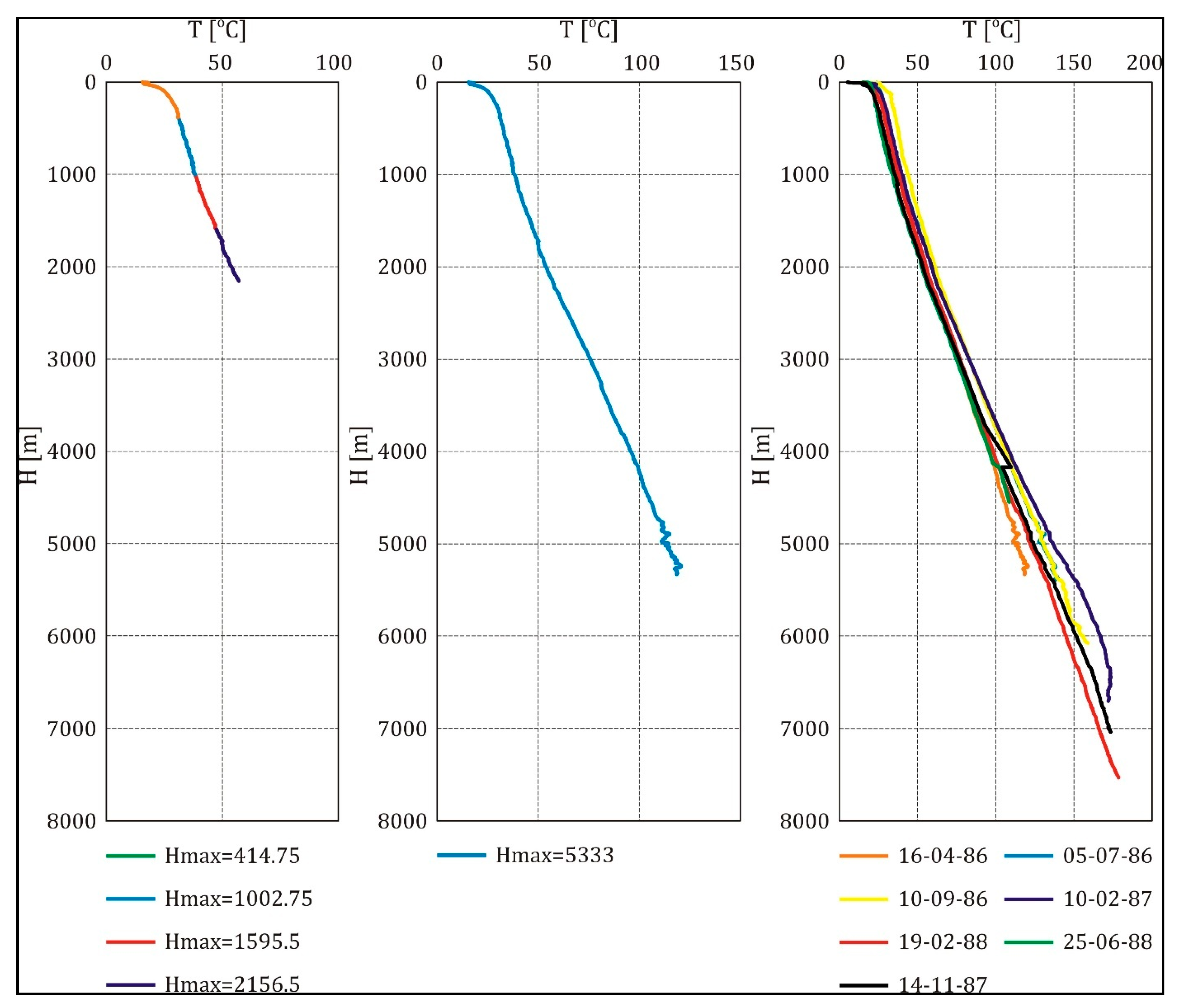
3.1. Temperature Measurements and Interpretation in GT-1, GT-2 and K-1 Boreholes

In the GT-1 borehole, in-depth interval 1894–2923 m, there was realized expanded set of logs comprising among others spectral gamma log, SGR, electric imaging with the use of X-tented Range Micro Imager (XRMI) device, and advanced sonic log using WSST tool. In this depth section, the Jurassic and Triassic clastic and carbonate formations were analyzed as the potential geothermal water reservoirs (Table 2). Production logging was realized in the GT-2 borehole, so direct measurements of outflow were available, together with the transient temperature log, Temp–PL curve (

Table 3. Results of various temperature measurements in GT-1 and GT-2 boreholes.

Bottom Hole Temperature, BHT					Production Log Temperature
GT-1			GT-2		GT-2
Depth [m]	BHT [°C]	Temp_Calc [°C]	Depth [m]	BHT [°C]	Depth [m]	Temp [°C]
20		8
403	24	22.99
1892.5	51	53.67	1922	50	2320	64.2
2351	62	67.58	2361	59
2769	71	75.07
2925.5	72	76.92

, Figure 2 and Figure 3). The presented cases were good examples to illustrate the usefulness of well logging in geothermal prospection and analyses. The temperature was measured as bottom-hole temperature (BHT) at the final depth points of logging runs (Table 3, Figure 2 and Figure 3). Based on the BHT measured values in the GT-1 borehole, calculated/aligned values of the temperature, Temp_calc were obtained using Horner plot [37,38]. The blue curve in Figure 2 may be the basis for the geothermal gradient determination. Figure 2 and Figure 3 also include a Temp meas log as the result of temperature logging in the GT-1 borehole after 13 days for getting temperature equilibrium.

Production logging was realized in the open hole GT-2 depth section 1928.5–2320.0 m. The water outflow log and temperature log in the dynamic conditions and GR log were realized (water outflow was unstable: 77–61.2 m³/h). The depth intervals, in which the maximal water outflow was observed, were determined in the interpretation. In the maximal water outflow intervals, a distinct increase in temperature was observed (Figure 4). Transient/temporary geothermal gradient calculated in the depth section of maximal outflow: 1933–1954 and 2149–2248.5 m was as equal to 1.74 and 1.46 °C/100 m, respectively.

In Poland, in older wells, it is possible to find temperature logs that are aimed to determine geothermal gradient. Such established temperature measurements are cost generating because the credible records of the orogeny temperature can be obtained after a significant time lapse between the end of the drilling process/mud circulation and temperature logging. The importance and difficulty of the process of obtaining the temperature balance in orogeny are illustrated in Figure 5. Three plots T vs. H present the results of the interval temperature measurements in the very deep borehole K-1, in south-eastern Poland. Results of the four sections of the temperature measurements are presented in the left plot. In the middle part, the results obtained on the same day as the results presented in the left plot are presented (the same date: 16 April 1988). Hmax represents the depth of the bottom of the borehole section at each run. The results obtained on the same day are repeatable. The right plot illustrates changes in temperature curves measured after the different number of days of time-lapse (different dates). Temperature vs. depth curve logged on 19 February 1988 (brown) is the most credible for geothermal gradient determination. The green curve, logged later (25 June 1988) in a shorter section covers the previous one. Differences in courses of the curves T vs. H measured in the different dates illustrate the importance of keeping a long time-lapse in temperature measurements.

3.2. Radiogenic Heat Calculation in GT-1 and S-1 Boreholes

Using the spectral gamma-ray (SGR) log in GT-1 borehole, in-depth section 1800–2906.8 m radiogenic heat, A in the selected formations was calculated using the formula (2). Simple statistics are presented (

Table 4. Simple statistics of the bulk density, spectral gamma ray, spectral gamma-ray (SGR) data and radiogenic heat in the selected formations in GT-1 borehole (Central Polish Anticlinorium), stratigraphy and adopted thermal conductivity.

Statistics	Stratigraphy/Formation/ Depth Interval [m], λ [W/m/°K]	RHOB [g/cm3]	U [ppm]	Th [ppm]	K [%]	A [μW/m3]
Min	J1, Ciechocinek Beds, 1820–1905, 2.47	2.21	0.19	1.14	1.34	0.262
Aver.		2.47	1.90	4.50	1.99	0.919
Hyp. Aver.		2.47	1.31	3.71	1.93	0.863
Max		2.67	3.75	7.79	3.29	1.334
Min	J1, Upper Sławęcice Beds 1905–1971, 2.80	2.20	0.06	0.25	1.03	0.196
Aver.		2.26	0.87	2.82	1.82	0.616
Hyp. Aver.		2.26	0.53	1.67	1.70	0.512
Max		2.51	3.79	9.48	3.58	1.520
Min	J1, Main Sławęcice Beds 1971–2132, 2.90	2.19	0.06	0.31	1.06	0.184
Aver.		2.27	1.09	3.80	1.58	0.618
Hyp. Aver		2.27	0.55	2.19	1.51	0.449
Max		2.49	5.41	11.14	2.76	1.882
Min	J1, Ksawerów and Kłodawa Beds 2132–2335.5, 3.72	2.19	0.01	0.24	0.82	0.150
Aver.		2.24	0.61	2.27	1.25	0.348
Hyp. Aver		2.24	0.34	1.54	1.22	0.291
Max		2.52	5.50	14.66	2.97	2.167
Min	TRe, Rhaetian, 2335.5–2528, 2.38	2.20	0.09	0.67	1.29	0.184
Aver.		2.39	1.99	7.31	3.03	1.071
Hyp. Aver		2.39	0.89	4.31	2.61	0.704
Max		2.85	6.79	25.37	4.38	3.202
Min	TK, Keuper, 2528–2755, 2.73	2.20	0.31	3.25	1.83	0.740
Aver.		2.49	3.01	9.17	3.42	1.588
Hyp. Aver		2.48	2.38	8.80	3.27	1.499
Max		2.95	8.29	12.89	4.99	3.024
Min	T2, Muschelkalk, 2755–2883.5, 3.75	2.21	0.54	0.98	0.45	0.348
Aver.		2.65	2.08	3.60	1.10	0.879
Hyp. Aver		2.64	1.92	3.04	1.01	0.817
Max		2.91	4.28	8.32	2.98	1.497
Min	T3, BunterSandstone, 2883.5–2906.8 (2925.4), 3.22	2.21	0.93	3.17	0.93	0.643
Aver.		2.59	1.59	6.75	1.59	1.231
Hyp. Aver		2.59	1.51	6.35	1.51	1.120
Max		2.70	2.69	10.11	2.69	1.603

) to show the variability of the parameters. Min and max values present the range of changeability. Arithmetic and hyperbolic averages are included to emphasize the large range and outliers’ presence. Both averages are almost the same in the bulk density but for other quantities, high differences are observed, leaning authors towards using hyperbolic average as more credible in the heat flow modelling.

Different values of radiogenic heat, A, were observed. Maximal values, reaching 2.167–3.202 μW/m³ are noted in the Jurassic (J1, Ksawerów and Kłodawa Beds) and Triassic (TRe, Rhaetian) formations. The highest average value of radiogenic heat was observed in the Triassic, TK, Keuper formation. High radiogenic heat in the J1, Ksawerów and Kłodawa Beds, built of thick-layered sandstones, resulted from the high thorium and potassium contents, in the Triassic mudstone, claystone formations were related to the highest uranium content. Results in Table 4 show that there is a distinctly visible relation between A and lithology.

Another example illustrating the differences in radiogenic heat in various lithostratigraphic formations was presented in the S-1 borehole, in the Carpathians, in the depth section 745–3500 m. Here, the Menilite Beds were the source formation of hydrocarbons [39]. They characterized the anomalously high values of radiogenic heat. All simple statistics of the Menilite Beds radiogenic heat were the highest in comparison to other formations. High ranges of quantities in the analyzed depth sections meant that formations were heterogeneous. Extremely high uranium content in the Menilite Beds was related to high organic matter content. High radiogenic heat was also characteristic for the First Variegated shales, but statistics are distinctly lower in comparison to the Menilite Beds, due to lower uranium content. Eocene Ciężkowice Sandstones are of lower radiogenic heat comparing to the Eocene Variegated shales due to lower uranium and thorium content. In the Paleocene and Cretaceous Istebna Shales and Sandstone, there was observed radiogenic heat lowering with depth.

The thermal conductivity of the Carpathians formation was adopted on the basis of the literature information and the archive results (

Table 5. Average thermal conductivity of the selected Carpathian rocks (K-1 borehole) [22,40].

Formation	λ [W/m°K]	Formation	λ [W/m°K]
Upper Krosno Beds	1.68	Inoceramus Beds	2.88
Lower Krosno Beds	2.36	Spas Beds	2.15–2.37
Menilite Beds	2.03	Kuźmina Sandstones	2.99
Hieroglyphic Beds and Variegated Shales	3.19	Stebnik Beds	2.41

) [22,32,40]. Archive data were obtained on the samples from the K-1 borehole using a similar experimental set for laboratory measurements of thermal conductivity like described in subchapter 2.4 [37]. Archive thermal conductivity values were the basis for the adoption of for heat flux and temperature modelling in the S-1 borehole (

Table 6. Simple statistics of the bulk density, spectral gamma ray, SGR data and radiogenic heat in the selected formations in S-1 borehole (the Carpathians), stratigraphy and adopted thermal conductivity.

Stratigraphy/Formation/ Depth Interval [m], Lithology, λ [W/m/°K]	RHOB [g/cm3]	U [ppm]	Th [ppm]	K [%]	A [μW/m3]
Oligocene, Krosno Beds,745–1692, fine grained sandstones—marly, limy and dolomitic, mudstone shales, 2.36	2.61	3.21	7.04	4.84	1.771
Lower Oligocene, Menilite Beds, 1692–1789.3, shales, fine grained sandstones—limy and dolomitic, 2.03	2.49	5.04	7.23	4.50	2.361
Lower Oligocene/Upper Eocene, Globigerine Beds, 1789.3–11795, marls with enclosure of shales, 1.25	2.19	3.21	9.13	5.75	1.656
Eocene, the First Variegated Shales, 1795–2041, shales, 2.10	2.28	3.92	12.06	5.99	2.085
Eocene, the First Ciężkowice Sandstone, 2041–2097.5, heterogranular sandstones, up to conglomerates, laminated with shales, 2.47	2.50	2.44	5.36	4.26	1.394
Eocene, the Second Variegated Shales, 2097.5–2108, shales, 2.15	2.36	3.29	9.18	5.64	1.840
Eocene, the Second Ciężkowice Sandstone, 2108–2181.3, hetero-granular sandstones, up to gravel facies, locally mudstone type, 2.48	2.55	2.26	4.47	3.80	1.249
Eocene, the Third and Forth Variegated Shales, 2181,3–2250, shale, 2.20	2.46	3.51	9.77	5.31	1.972
Paleocene, Upper Istebna Shales, 2250–2734, shales—limy, clayey, partially marly, 2.00	2.36	0.22	9.62	3.58	1.499
Paleocene, Upper Istebna Sandstones, 2734–2917, fine and middle grained sandstones, laminated with shales, 2.48	2.46	0.25	5.47	3.13	1.114
Paleocene, Lower Istebna Shales, 2917–2948, shales—limy, clayey, partially marly, 2.00	2.33	0.26	6.27	3.38	1.120
Upper Cretaceous, Lower Istebna Sandstone, 2948–3500, fine grained sandstones to mudstones, laminated with shales, 2.50	2.48	0.25	4.49	2.97	0.998

).

Data in Table 4 and Table 6 reveal the differences in radiogenic heat only on the basis of bulk density and uranium, thorium and potassium contents in boreholes GT-1 and S-1. The depth of the boreholes is more or less similar but the age of drilled formation and lithology is different. In the GT-1 borehole, the drilled formations are older compared to the S-1 borehole. The GT-1 borehole was drilled to recognize heat productivity from the formation waters. The most perspective as regards average radiogenic heat turned out the Jurassic and Triassic formations. In the Carpathians, the general level of radiogenic heat is higher. Radiogenic heat, A (Table 4 and Table 6), together with the adopted thermal conductivity values, were the basis for heat flow and temperature modelling.

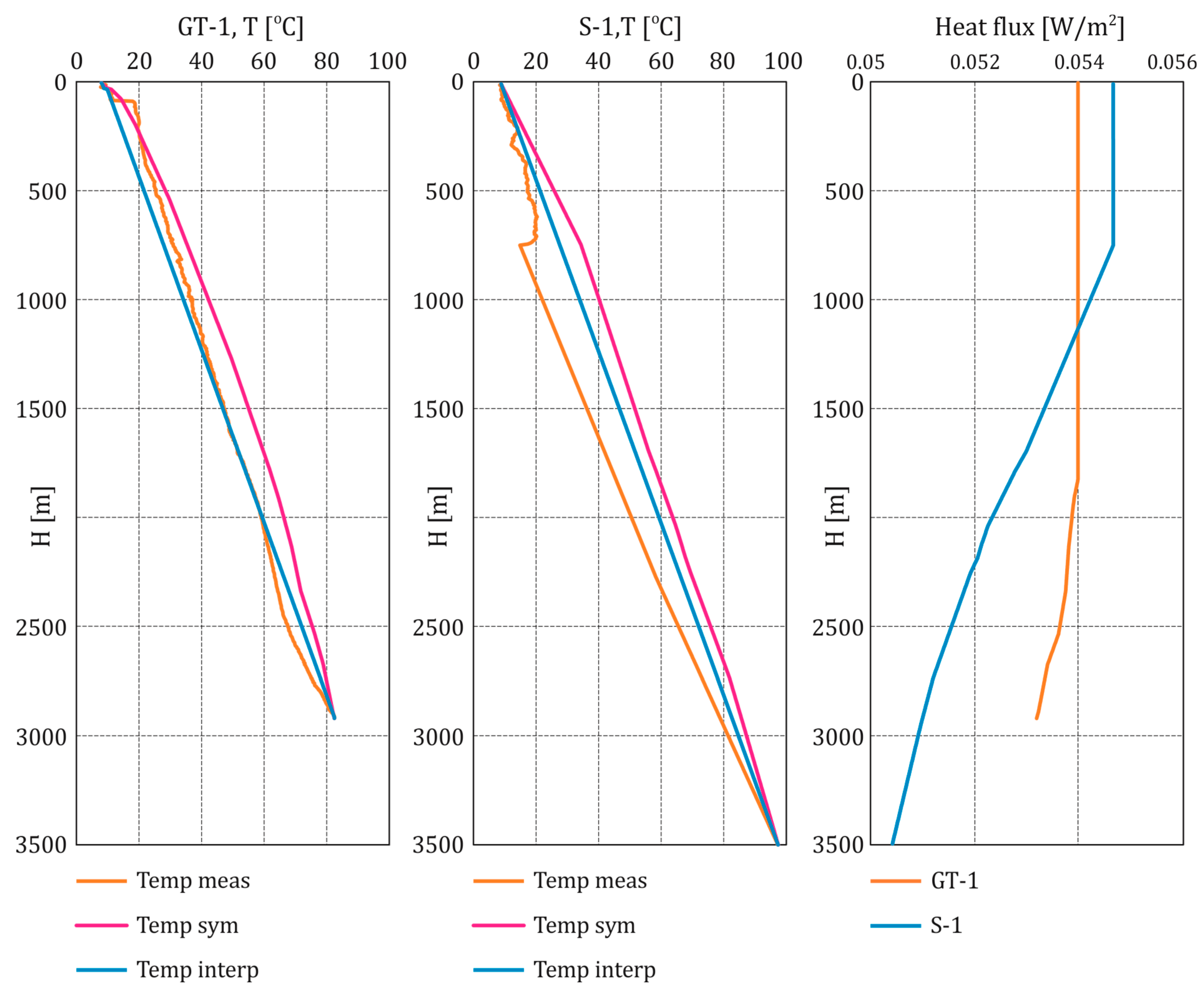
3.3. Heat Flow and Temperature Modelling

The elementary balance method [41] was applied for modelling using finite difference solution for calculations. One-dimensional balance conditions for inner cells were adopted on the basis of Equation (12) for heat and (13)—temperature:

$${\dot{Q}}_{\left(x-1\right)\to x}+{\dot{Q}}_{\left(x+1\right)\to x}+{\dot{Q}}_{vx}=0$$

(12)

$$T_x=\frac{T_{x-1}+T_{x+1}+\frac{{\dot{q}}_{vx}{\left(\Delta x\right)}^2}{{\lambda }_x}}{2}$$

(13)

where: ${\dot{Q}}_{\left(x-1\right)\to x}$, ${\dot{Q}}_{\left(x+1\right)\to x}$ and ${\dot{Q}}_{vx}$—heat flowing from the upper and lower cells and generated in the modelled cell, respectively, $T_{x-1}$, $T_{x+1}$, $T_x$—temperature in the upper, lower and modelled cells, respectively, ${\dot{q}}_{vx}$—unit heat generated in the modelled cell, $\Delta x$—depth step, ${\lambda }_x$—heat conductivity in the modelled cell.

For the marginal cells, where the temperature of the neutral layer and the bottom hole temperature, BHT is known, there were used the Dirichlet boundary conditions [42,43]. Thermal conductivity was adopted on the basis of archival laboratory measurements [22], literature [32], known lithology and depth (Table 4 and Table 6). Comparison of the modelling results revealed some differences (

Table 7. Comparison of the heat flow modelling results in GT-1 and S-1 boreholes.

Description	Heat Flux [mW/m2]		Description	Thermal Power [mW/m2]
	GT-1	S-1		GT-1	S-1
Earth surface heat flux			Thermal power in the column of the base area equal to 1m2	0.794	4.264
Without radiogenic heat	53.89	53.41
with radiogenic heat	53.98	54.65
Difference	0.09	1.24	Thermal power ratio (S-1/GT-1)	5.370
Heat flux at the bottom of the borehole	53.19	50.41
Difference between heat flux in the neutral layer and borehole bottom	0.70	2.00	Difference heat flux ratio (S-1/GT-1)	2.857

). The difference between the Earth surface heat flux (neutral layer) and the borehole bottom fluxes is almost three times higher in S-1 in comparison to GT-1. Thermal power in the S-1 borehole is more than 5 times higher than in GT-1. This allows us to conclude that the generated radiogenic heat in the Carpathians contributed to the increase of the local Earth heat flux to a greater extent than in the Central Polish Anticlinorium.

The modelling results show that the influence of the radiogenic heat generated inside the analysed rock formation is not very big. Radiogenic heat generated in the upper layers reduces the heat flux from the layers below, while the surface heat flux is slightly increased. Higher values of the Earth surface fluxes modelled including radiogenic heat and difference between modelled heat fluxes at the borehole bottom and surface show that it is valuable to use the available data (SGR and bulk density). Temperature vs. depth plots in GT-1 and S-1 boreholes (Figure 6) as the results of the modelling (Temp sym) showed the different courses in comparison to the measured curves (Temp meas). The linear interpolation provided more credible curves (Temp interp).

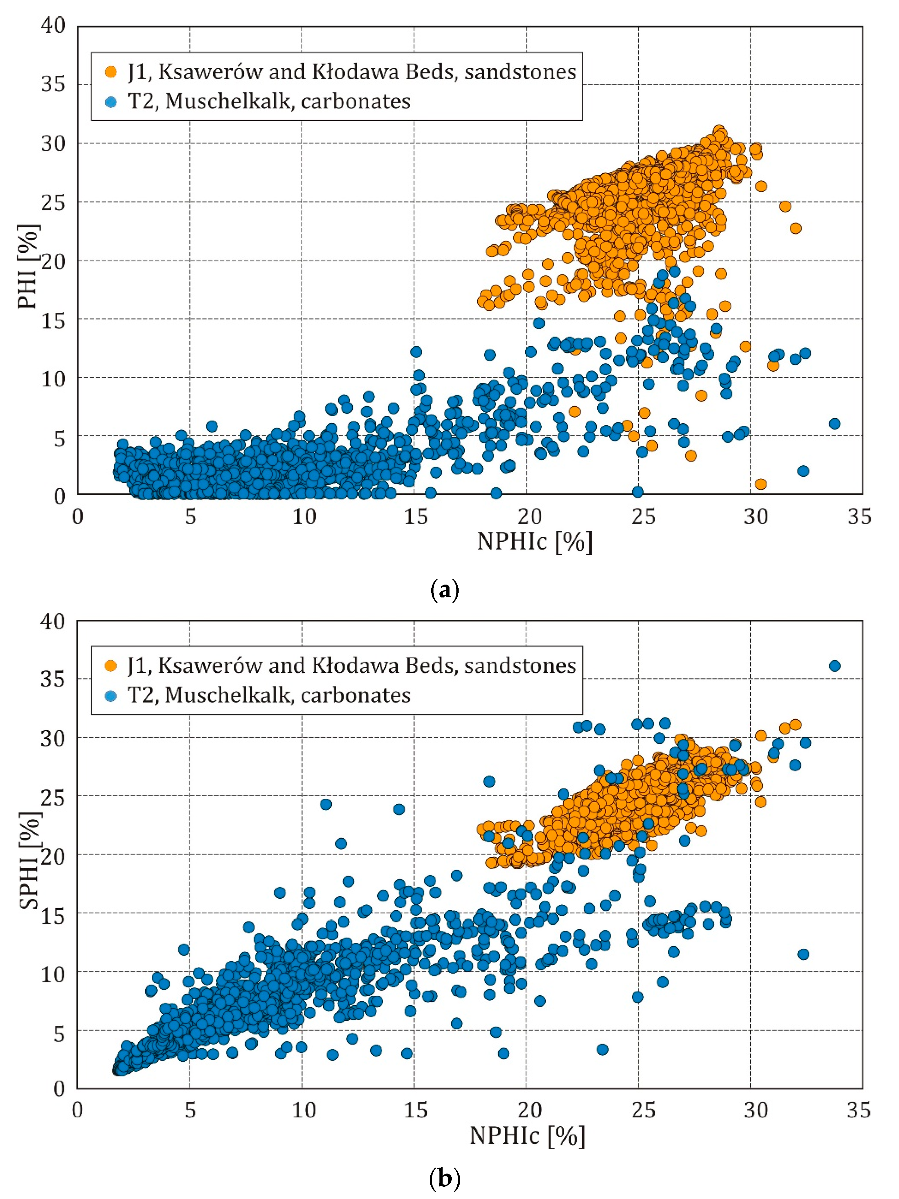
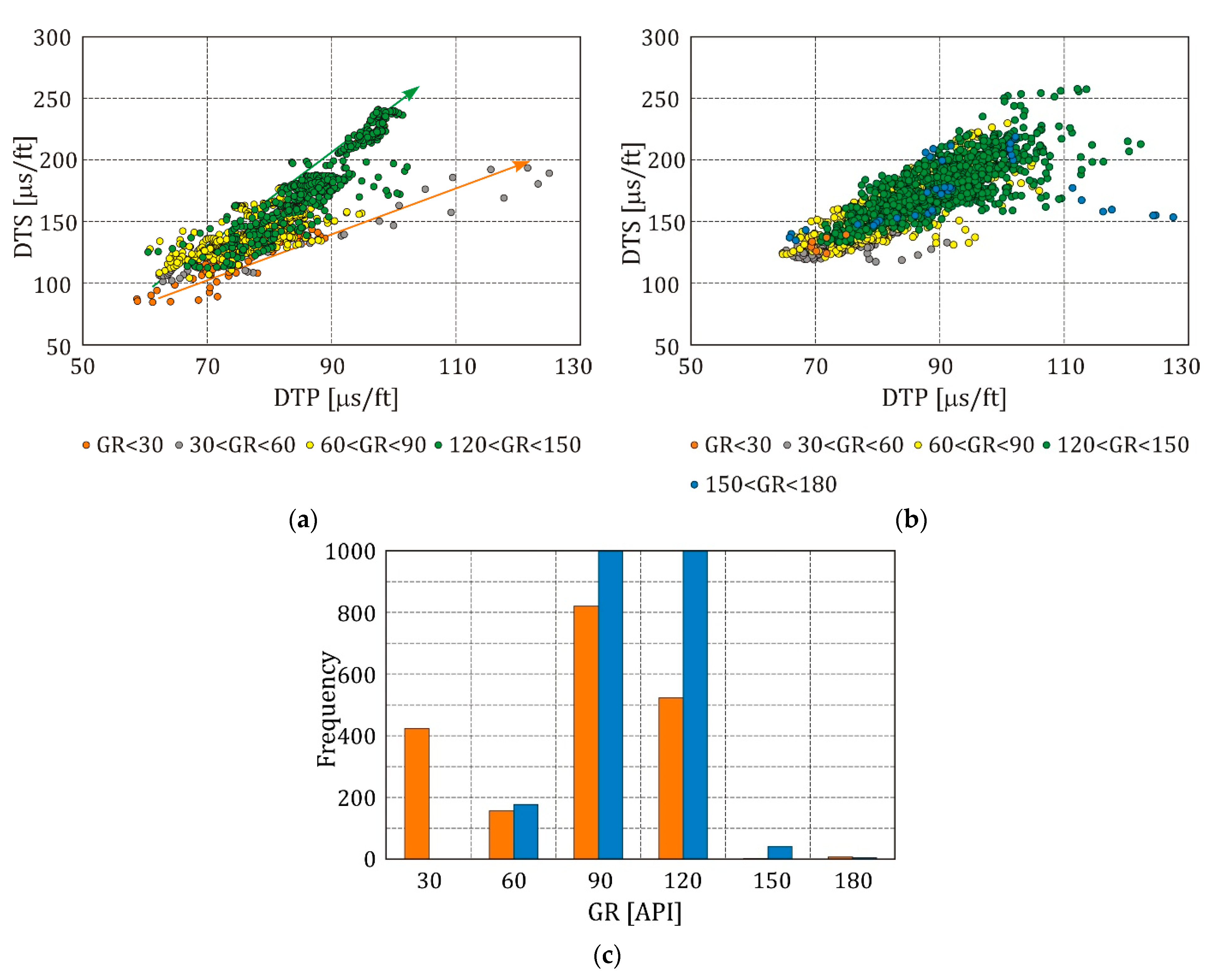
3.4. Examples of the Comprehensive Interpretation of Well Logs Used in Petrophysical Characterization of Reservoir Rocks

Standard comprehensive interpretation of well logs made in the computer systems used in Poland enables porosity and lithology determination. The number of independent logs running in the borehole always limited the number of mineral components in which volumes could be calculated. So, it is very important to make as many as possible logs measuring different parameters to obtain as extend information as possible. Total porosity, PHI from the comprehensive interpretation of logs is the most credible value, much more reliable than values calculated from individual logs (RHOB, NPHI, DT, formulas (3) and (4)). PHI is not quite free from the matrix influence, but adopting matrix parameters for density, neutron and sonic logs causes that total porosity, PHI could be considered as an average value including features of each logging. For quick lithology characterization of the potential water reservoirs in the GT-1 borehole cross-plotted comparison of the various porosity logs were considered (Figure 7a,b). In the PHI vs. NPHIc plot total porosity, PHI of the Jurassic J1 sandstones revealed higher values than Triassic T2 carbonates (Table 2). Shaliness of sandstones explained data scattering. PHI of the Triassic T2 carbonates was generally lower than Jurassic J1 sandstones, scattering of data was related to intergranular porosity, fissures and fractures of carbonates. PHI of carbonates was distinctly lower than NPHIc, In sandstones, PHI and NPHIc were close ones to another. A similar but not so distinct difference between SPHI and NPHIc in carbonates was visible in Figure 7b. SPHI and NPHIc of sandstones are focused around the diagonal. NPHI is considered as higher than real porosity due to various hydrogen location in rock while SPHI is lower than real PHI due to the shorter supposed trajectory of the elastic wave in comparison to the real one.

Primary lithology recognition was also possible based on other logs. After processing results of Wave Sonic log with dipole source in GT-1 borehole slowness of elastic P- and S-waves (DTP and DTS) were determined in-depth section 2335.0–2752.0 m comprising the Rhaetian and Keuper formations (Figure 8a,b). In Figure 8a two branches are observed—one in more sandy formation and the second—in more shaly one. The position of the branches is determined by DTP and DTS values. GR histograms (added in Figure 8c) distinctly differentiate between more shaly Keuper and more sandy Rhaetian formations. Histograms are a quick and effective statistical tool, good for illustrating differences in shaliness. Numerical data for histograms are presented in

Table 8. Numerical data for histograms in Figure 8c.

GR Class [API]	TRe, Rhaetian	TK, Keuper
	Number od Data
30	424	0
60	156	177
90	820	1010
120	523	1009
150	2	41
180	6	4

. It is visible that shaliness is present in the sandy Rhaetian layers but on the lower level compared to the Keuper. In the deeper depth section, 2771.0–2912.0 m, comprising Muschelkalk and Bunter Sandstone slowness of P-, S- and Stoneley waves (DTP, DTS and DTST) were determined from the Full Wave Sonic Log (Figure 9a,b). Similar lithology of Rhaetian and Keuper built with sandstone, mudstone and claystone with the admixture of calcareous and dolomitic substance was differentiated using shaliness and slowness, representing the base data for porosity calculation. Stoneley wave slowness provided qualitative information on permeability and enabled differentiation between hard and porous carbonates.

Electric imaging in GT-1 borehole, made using XRMI (Halliburton) device, was the newest version of the micro-resistivity measurements realized on the borehole wall. Six Electrode Dipmeter, SED (Halliburton) probe, providing six micro-resistivity logs was the prototype of the modern electric imaging, which now provides with 125 micro-resistivity logs. The basic goal of dipmeter logging was to show dips and azimuths of the inter-beds in clastic formations. XRMI device turned out to be more advanced in interpretation enabling the additional calculation of natural and induced fractures. Two samples of electric imaging and dipmeter plots from the Jurassic J1 clastic formation—the Ksawerów and Kłodawa Beds built of thick sandstone layers (Figure 10) and T2 carbonates of the Muschelkalk (Figure 11) are presented to show similarities and differences in the illustrations. Bedding is distinctly visible in the static image of XRMI and Resistivity Map from SED. Dips, presented as coloured vectors, occupied range 0–30°. Coloured azimuth roses showed the dominating dips and azimuths. Groups of fractures resulted from processing of XRMI images. In SED processing different parameters were adopted: (a) 0.5 m × 0.25 m × 45 or (b) 1 m × 0.5 m × 45 or (c) 2 m × 1 m × 75 to reveal more (a) or less (c) details in bedding. Colours in the Static image and Resistivity Map are related to lower (darker) and higher (lighter) resistivity. Information on mineral components—shaliness (darker layers) decreasing porosity and permeability is important in geothermal water potential estimating in the reservoir. In carbonates, dips covered lower range than in clastics, dominating dips were lower than 10°. Carbonate structures were observed in the upper part of the section, where the high scattering of dips and azimuths were noted. Outcomes of electric imaging (also acoustic imaging) together with the novel sonic log results provide unique information on the directions of low and high orogeny pressure useful in artificial fracturing planning.

3.5. Nuclear Magnetic Resonance—A Source of Expanded Information on Porosity

Nuclear Magnetic Resonance logging and laboratory experiments distinctly differentiate between total and effective/dynamic porosity and show variability between water in micropores, bound and free water. It is a safety method from the environmental protection viewpoint, useful in qualitative illustration and quantitative calculation of porosity and permeability. Results of NMR logging (made by Halliburton for PGNiG SA) in the Miocene shaly sandstones and Jurassic carbonates in L-4 borehole (Carpathian Foredeep) reveal the quick look possibility to recognize the position of water in pore space (Figure 12). In both parts of the plot, in the first track the measured depth is presented, in the second—three resistivity curves are shown in the same logarithmic scale. There is a difference in the resistivity level—low in the shaly-sandstone, high in carbonate. LLS (blue) and LLD (red) curves (shallow and deep laterologs, respectively) almost cover one another, MSFL log (black) presents the lowest value in the upper part due to the caverns that occurred in the soft shaly–sandy formation. Small differences between MSFL and LLS/LLD curves in the carbonate part show low porosity filled with formation water. The third and fourth tracks show relaxation times, T2 and T1 distributions. Rose and blue lines in these plots mean cut-offs for the micropore and bound water spaces. There are visible differences in the cut-offs for the shaly–sandy and carbonate formations. Cut-off values are adopted based on the lab experiments and interpreter experience [44,45]. In both plots, in the last track, there are presented coloured areas. Micropores are marked in green, free fluid index, i.e., movable water—in yellow. In carbonates, there is no water bound in clays, but microporosity is observed. T2 and T1 signals registered in low times are related to microporosity.

Permeability, K can be calculated on the basis of NMR results using for instance Coates formula (13) [46] in which there are used the following quantities obtained from NMR measurement: K_{p NMR}—total porosity from NMR, Kp1—volume of irreducible water, Kp2—volume of capillary water and Kp3—volume of free water. In well-logging interpretation in Poland, there is also the popular Zawisza formula [47], (14) in which effective porosity K_ef and irreducible water saturation, S_wi are used.

$$\mathrm{K}{\_}_{\mathrm{C}}={\left(\mathrm{C}\times {\mathrm{K}}_{\mathrm{PNMR}}\right)}^4\times {\left(\frac{\mathrm{Kp}3}{\mathrm{Kp}1+\mathrm{Kp}2}\right)}^2$$

(14)

$$\mathrm{K}{\_}_{\mathrm{ZAW}}=\mathrm{C}\times {\mathrm{K}}_{\mathrm{ef}}{}^{\mathrm{C}1}\times {\left(1-{\mathrm{S}}_{\mathrm{wi}}\right)}^2$$

(15)

The presented formulas (13 and 14) are empirical ones and the interpreter is obliged to adopt suitable constants (C, C1). Discrepancies between $\mathrm{K}{\_}_{\mathrm{C}}$ and $\mathrm{K}{\_}_{\mathrm{ZAW}}$ are frequently observed but they are treated as a source of additional information taking into account that NMR identifies hydrogen presence in various parts of pore space and mineral crystals and ${\mathrm{K}}_{\mathrm{ef}}$ and ${\mathrm{S}}_{\mathrm{wi}}$ are determined from resistivity logs.

4. Summary

The goal of the paper was to present the well logging possibility of use in geothermal resources recognition and characterization. Thanks to the extended development of well logging devices for measurements and interpretation techniques a great variety of petrophysical parameters—porosity, permeability, fracturing, mineral composition—the elasticity of orogeny and mineralization of formation water can be credibly determined. The authors would like to underline possible cooperation between well log analysts and petrophysicists and specialists on geothermal energy to increase efficient utilization of the technical solutions known from the HC deposits prospection and evaluation. Well logging measurement technics and methods of processing and statistical elaboration of data are successfully used in several areas, among others in hydrogeology, for evaluating formation shaliness in groundwater studies [48]. Another example is uranium mining, where gamma-ray spectroscopy measurements are the input for the orogeny condition simulations [49]. Additionally, non-destructive laboratory and borehole measurements based on gamma radiation of rocks are popular for obtaining indispensable information on bulk density in mining exploitation [50]. The interest in radiogenic heat calculations based on spectral gamma-ray measurements, also using aero-geophysical acquisition, is also observed in Africa to determine the spatial distribution of radiogenic heat and temperature within the lithosphere, thanks to the relative ease of obtainment and cheap data [51,52]. Additionally, geothermal heat pump development indicates that it is worthwhile to pay attention to the measurements and calculation of radiogenic heat in boreholes in the recognized lithological profiles, as it is a part of heat supplying pumps [53,54]. Petrophysical characteristics of individual formations and correlation of reservoir horizons in geothermal provinces using well logging were also practiced in Poland [17]. The authors treated the research results and selected encouraging examples as a kind of promotion of highly developed well logging methods and methodologies in novel applications in the area of great importance for the sustainable development of the environment.

Only selected methods were discussed but an existing variety of other methodologies could provide additional information on pressure gradient influencing heat flow or detailed information on the salinity of formation water. It is worth underlining that necessary information for geothermal aims is mostly gathered in well logging archive data and could be accessible with minimal costs. Archive data could be effectively used in further analyses and complete the new measurements. For investors, knowledge of the parameters possible to be determined from logs to order proper measurements is important.

Many petrophysical parameters obtained from well logs can be also obtained in laboratory experiments with the same physical basis as well logging. Despite their point character, direct laboratory measurements construct the platform confirming well-logging data, continuous and relatively cheap but indirect and obtained in boreholes in a special environment.

5. Conclusions

Reservoir parameters considered in hydrocarbon deposits and geothermal resource prospection and characterization can be determined from well logs. Archive and contemporary well-log data are useful sources of porosity, fracturing, permeability, mineral composition (shaliness) and elastic properties of rocks. Various temperature logs and spectral gamma-ray logs play special roles. The first ones provide information on the orogeny and thermal water temperature and geothermal gradient, and the second enable radiogenic heat calculation and determination of shaliness, deeply influencing porosity and permeability.

Porosity is obtained from logs with a different physical basis, so the differences in results are the source of additional information. Three resistivity logs of the different radius of investigation give quick recognition of reservoir formation and precisely inform on effective porosity. Nuclear magnetic resonance credibly differentiates between total and dynamic porosity. Reliable effective/dynamic porosity values are the basis for physical permeability determination. Electric imaging provides quick information on the fracturing and, together with the modern acoustic logs, enriches the characteristics of the rock on the elasticity of orogeny. Precise information on the thickness of the reservoir, porosity and permeability enables credible calculation of geothermal water resources.

Thermal conductivity is an important parameter in geothermal investigations. Laboratory measurements of this parameter are relatively simple, necessary equipment is not very complicated and expensive and rock specimens can be obtained without great effort. Another way to obtain thermal conductivity is the calculation based on mineral composition, which is available from the comprehensive interpretation of well logs. Temperature and radiogenic heat, together with thermal conductivity, are the input parameters for surface heat flux modelling, representing important information in planning ecological energy sources.

References

1. Lowrie, W. Fundamentals of Geophysics, 2nd ed.; Swiss Federal Institute of Technology, Zürich, Cambridge University Press: Cambridge, UK; New York, NY, USA; Melbourne, Australia; Madrid, Spain; Cape Town, South Africa; Singapore; São Paulo, Brazil, 2007; pp. 207–250. [Google Scholar]
2. Serra, O. Fundamentals of Well-Log Interpretation—The Acquisition of Logging Data; Elsevier Science Publishers B.V.: Amsterdam, The Netherlands, 1984; p. 435. ISBN 0-444-42132-7. [Google Scholar]
3. Darling, T. Well Logging and Formation Evaluation; Elsevier: Amsterdam, The Netherlands; Boston, MA, USA; Heidelberg, Germany; London, UK; New York, NY, USA; Oxford, UK; Paris, France; San Diego, CA, USA; San Francisco, CA, USA; Singapore; Sydney, Australia; Tokyo, Japan, 2005; p. 336. [Google Scholar]
4. Asquith, G.B.; Krygowski, D. Basic Well Log Analysis, 2nd ed.; AAPG: Tulsa, OK, USA, 2004; pp. 1–244. [Google Scholar]
5. Ellis, D.V.; Singer, J.M. Well Logging for Earth Scientists, 2nd ed.; Springer: Dordrecht, The Netherlands, 2008; p. 692. ISBN 978-1-4020-3738-2. [Google Scholar]
6. Janowski, M. The possibilities of using geothermal waters for recreational and balneological purposes-technical-economic aspect. Tech. Poszuk. Geol. 2011, 1, 257–265. [Google Scholar]
7. Chowaniec, J.; Poprawa, D.; Witek, K. Występowanie wód geotermalnych w polskiej części Karpat. Prz. Geol. 2001, 49, 734–742. [Google Scholar]
8. Dowgiałło, J. The Sudetic geothermal region of Poland. Geothermics 2002, 31, 343–359. [Google Scholar] [CrossRef]
9. Górecki, W.; Ciągło, J. Perspektywiczne lokalizacje dla zagospodarowania energii geotermalnej na Niżu Polskim. Tech. Poszuk. Geol. 2007, 47, 35–40. [Google Scholar]
10. Chowaniec, J. Studium hydrogeologii zachodniej części Karpat polskich. Biul. Państw. Inst. Geol. 2009, 434, 1–98. [Google Scholar]
11. Górecki, W.; Hajto, M.; Strzetelski, W.; Szczepański, A. Dolnokredowy oraz dolnojurajski zbiornik wód geotermalnych na Niżu Polskim. Prz. Geol. 2010, 58, 589–593. [Google Scholar]
12. Hajto, M. Geothermal potential of the Outer Western Carpathians. Tech. Poszuk. Geol. 2011, 50, 37–49. [Google Scholar]
13. Górecki, W.; Hajto, M.; Szczepański, A.; Oszczypko, N. (Eds.) Atlas Zasobów Wód i Energii Geotermalnej Karpat Zachodnich; AGH UST FGGEP Department of Fossil Fuels, Ministry of Environment: Krakow, Poland, 2011; p. 772.
14. Sapińska-Śliwa, A. History of Exploitation of Thermal Waters in Uniejów. Biuletyn Uniejowski 2012, 1, 63–76. [Google Scholar]
15. Górecki, W.; Sowiżdżał, A.; Jasnos, J.; Papiernik, B. (Eds.) Atlas Geotermalny Zapadliska Przedkarpackiego; AGH UST FGGEP Department of Fossil Fuels: Krakow, Poland, 2012; p. 418.
16. Górecki, W.; Hajto, M.; Sadurski, A.; Szczepański, A. (Eds.) Atlas Zasobów Geotermalnych Na Niżu Polskim—Formacje Paleozoiku; KrakówAGH UST FGGEP Department of Fossil Fuels: Krakow, Poland, 2006; p. 240.
17. Sowiżdżał, A.; Papiernik, B.; Machowski, G.; Hajto, M. Characterization of petrophysical parameters of the Lower Triassic deposits in prospective location for Enhanced Geothermal System (central Poland). Geol. Q. 2013, 57, 729–744. [Google Scholar] [CrossRef] [Green Version]
18. Bujakowski, W.; Tomaszewska, B. (Eds.) Atlas of the Possible use of Geothermal Waters for Combined Production of Electricity and Heat Using Binary System in Poland; MEERI PAS: Krakow, Poland, 2014; p. 305. [Google Scholar]
19. Górecki, W.; Sowiżdżał, A.; Hajto, M.; Wachowicz-Pyzik, A. Atlases of geothermal waters and energy resources in Poland. Environ. Earth Sci. 2015, 74, 7487–7495. [Google Scholar] [CrossRef] [Green Version]
20. Kępińska, B. (Ed.) Energia Geotermalna-Podstawa Niskoemisyjnego Ciepłownictwa, Poprawy Warunków Życia I Zrównoważonego Rozwoju-Wstępne Studia Możliwości Dla Wybranych Obszarów W Polsce. Raport z Wizyt Studyjnych. 2017, pp. 18–40. Available online: http://www.eeagrants.agh.edu.pl/wp-content/uploads/2017/12/EOG-Raport-GeoHeatPol-2017.pdf (accessed on 21 November 2020).
21. Górecki, W.; Hajto, M.; Augustyńska, J.; Jasnos, J. (Eds.) Geothermal Atlas of the Eastern Carpathians; AGH UST FGGEP, Department of Fossil Fuels: Krakow, Poland, 2013; p. 791.
22. Malata, T.; Żytko, K. (Eds.) Profile Głębokich Otworów Wiertniczych PIG Kuźmina 1; Polish Geological Institute: Warsaw, Poland, 2006; Volume 110, p. 70. [Google Scholar]
23. Sokołowski, J. Dokumentacja geosynoptyczna otworu geotermalnego Bańska IG-1. Geosynop. I Geotermi. 1992, 1, 1–119. [Google Scholar]
24. Dowgiałło, J. The Sudetic geothermal region of Poland—New findings and further prospects. In Proceedings of the World Geothermal Congress, Kyushu-Tohoku, Japan, 28 May–10 June 2000. [Google Scholar]
25. Wójcicki, A.; Sowiżdżał, A.; Bujakowski, W. Evaluation of Potential, Thermal Balance and Prospective Geological Structures for Needs of Closed Geothermal Systems (Hot Dry Rocks) in Poland; Ministry of Environment: Warsaw, Poland; Krakow, Poland, 2013; p. 246.
26. Rybach, L. (Ed.) Radioactive Heat Production; a Physical Property Determined by the Chemistry in the Physical and Chemistry of Minerals and Rocks; John Wiley & Sons Inc.: Hoboken, NJ, USA, 1976. [Google Scholar]
27. Rybach, L. Determination of heat production rate. In Handbook of the Terrestial Heat Flow Density Determination; Kluwer Academic Publishers: Dordrecht, The Netherlands, 1988; pp. 125–142. [Google Scholar]
28. Bücker, C.; Rybach, L. A simple method to determine heat production from gamma ray logs. Mar. Petrol. Geol. 1996, 13, 373–375. [Google Scholar] [CrossRef]
29. Allen, D.; Carry, S.; Freedman, B.; Andreani, M.; Klopf, W.; Badry, R.; Flaum, C.; Kenyon, B.; Kleinberg, R.; Gossenberg, P.; et al. How to Use Borehole Nuclear Magnetic Resonance. Oceanogr. Lit. Rev. 1998, 3, 586–587. [Google Scholar]
30. Coates, G.R.; Xiao, L.; Prammer, M.G. NMR Logging Principles & Applications; Halliburton Energy Services: Houston, DE, USA, 1999; p. 235. [Google Scholar]
31. Szewczyk, J.; Gientka, D. Terrestrial heat flow density in Poland—A new approach. Geol. Q. 2009, 53, 125–140. [Google Scholar]
32. Schön, J.H. Physical Properties of Rocks: Fundamentals and Principles of Petrophysics, 2nd ed.; Elsevier: Amsterdam, The Netherlands, 2015; p. 497. ISBN 978-0-08-100404-3. [Google Scholar]
33. Doveton, J.; Förster, A.; Merriam, D.F. Predicting thermal conductivity from petrophysical logs: A Midcontinent Paleozoic case study. In Proceedings of the IAMG’97, CIMNE, Barcelona, Spain, 22–27 September 1997. [Google Scholar]
34. Janowski, M. Heating pomp as ecologic heat source? In Proceedings of the Ogólnopolski Kongres Geotermalny Geotermia w Polsce-doświadczenia, stan aktualny, perspektywy rozwoju, Radziejowice, Poland, 17–19 October 2007. [Google Scholar]
35. Ciapała, B.; Janowski, M. Shallow bedrock layers temperature local variability—Trivia or touchstone? historic view and possible application. In Proceedings of the VI Polish Geothermal Congress, Zakopane, Poland, 23–25 October 2018; p. 21, ISBN 978-83-65874-02-3. [Google Scholar]
36. Available online: http://www.geofizyka.agh.edu.pl/en/laboratory-of-elastic-and-mechanical-property/ (accessed on 21 November 2020).
37. Corrigan, J. 2003-Correcting Bottom-Hole Temperature Data. Available online: https://www.zetaware.com/utilities/bht/horner.html (accessed on 21 November 2020).
38. Pasquale, V.; Verdoya, M.; Chiozzi, P. Geothermics, Heat Flow in the Lithosphere, 2nd ed.; Springer: Berlin/Heidelberg, Germany, 2017; p. 138. ISBN 978-3-319-52083-4. [Google Scholar]
39. Dziadzio, P.S.; Matyasik, I.; Garecka, M.; Szydło, A. Lower Oligocene Menilite Beds, Polish Outer Carpathians: Supposed deep-sea flysch locally reinterpreted as shelfal, based on new sedimentological, micropalaeontological and organic-geochemical data. Pr. Naukowe Inst. Naft. i Gazu 2016, 120. [Google Scholar] [CrossRef]
40. Plewa, M. Wyniki Badań Cieplnej Przewodności Właściwej I Gęstości Powierzchniowego Strumienia Cieplnego Ziemi W Otworze Kuźmina 1 Na Podstawie Pomiarów Laboratoryjnych Próbek Skał; W: Program poszukiwań fałdów wgłębnych w Karpatach w oparciu o wyniki super głębokiego wiercenia Kuźmina 1; Centr. Arch. Geol. Państw. Inst. Geol., Oddz. Karpacki.: Kraków, Poland, 1989. [Google Scholar]
41. Nagórski, Z. Modelowanie Przewodzenia Ciepła Za Pomocą Arkusza Kalkulacyjnego; Oficyna Wydawnicza Politechniki Warszawskiej: Warszawa, Poland, 2001; pp. 114–116. [Google Scholar]
42. Nagórski, Z. Modelowanie Przepływu Ciepła Metodą KM3R; Oficyna Wydawnicza Politechniki Warszawskiej: Warszawa, Poland, 2014; pp. 186–191. ISBN 978-83-7814-085-6. [Google Scholar]
43. Ciapała, B.; Hajto, M.; Janowski, M. Analytical models of the borehole heat exchanger ground heat source exploitation (GeoPLASMA-CE). In Proceedings of the VI Polish Geothermal Congress, Zakopane, Poland, 23–25 October 2018; p. 11, ISBN 978-83-65874-02-3. [Google Scholar]
44. Puskarczyk, E. Ocena Własności Zbiornikowych Skał Przy Wykorzystaniu Zjawiska Magnetycznego Rezonansu Jądrowego. Ph.D. Thesis, AGH University of Science and Technology, Main Library, Krakow, Poland, 2011; p. 135. [Google Scholar]
45. Romero, P.A. NMR Rock Typing. 2016, p. 5. Available online: http:http://www.geoneurale.com/documents/RockTypingusingNMR1.pdf (accessed on 21 November 2020).
46. Coates, G.R.; Dumanoir, J.L. A New Approach to Improved Log Derived Permeability. The Log Analyst, January–February 1974; 17. [Google Scholar]
47. Zawisza, L. Simplified method of absolute permeability estimation of porous beds. Arch. Min. Sci. 1993, 38, 343–352. [Google Scholar]
48. Szabó, N.P.; Dobróka, M.; Turai, E.; Szűcs, P. Factor analysis of borehole logs for evaluating formation shaliness: A hydrogeophysical application for ground water studies. Hydrogeol. J. 2014, 22, 511–526. [Google Scholar] [CrossRef]
49. Marchais, T.; Pérot, B.; Carasco, C.; Allinei, P.-G.; Chaussonnet, J.-L.; Toubon, H. Gamma-ray spectroscopy measurements and simulations for uranium mining. EPJ Web Conf. 2018, 170. [Google Scholar] [CrossRef] [Green Version]
50. Ross, P.-S.; Bourke, A. High-Resolution Gamma Ray Attenuation Density Measurements on Mining Exploration Drill Cores, Including Cut Cores. J. Appl. Geophys. 2018, 136, 262–268. [Google Scholar] [CrossRef] [Green Version]
51. Abbady, A.G.E.; Al-Ghamdi, A.H. Heat production rate of radioactive elements of granite rocks in north and southeastern Arabian shield Kingdom of Saudi Arabia. J. Radiat. Res. Appl. Sci. 2018, 11, 281–290. [Google Scholar] [CrossRef] [Green Version]
52. Aisabokhae, J.; Adeoye, M. Spatial distribution of radiogenic heat in the Iullemmeden basin—Precambrian basement transition zone, NW Nigeria. Geol. Geophys. Environ. 2020, 46, 239–250. [Google Scholar]
53. Lund, J.; Sanner, B.; Rybach, L.; Curtis, R.; Hellström, G. Geothermal (ground–source) heat pumps, a world overview. GHC Bull. 2004, 25, 1–10. [Google Scholar]
54. Rybach, L.; Eugster, W.J. Sustainability aspects of geothermal heat pumps. In Proceedings of the 27th Workshop on Geothermal Reservoir Engineering, Stanford University, Stanford, CA, USA, 28–30 January 2002; pp. 57–64. [Google Scholar]
Figure 1. Location of boreholes in the study (GT-1, GT-2, K-1, S-1 and L-4) on the background of geological units in Poland; source: e-podreczniki.pl—modified.
Energies 14 00850 g001
Figure 2. Temperature vs. depth from bottom hole temperature (BHT) measurements and Temp Log in GT-1; black points—BHT measurements, orange points—calculated temperature, violet line—Temp meas log.
Energies 14 00850 g002
Figure 3. Temperature vs. depth from BHT measurements in GT-1 and GT-2 boreholes, Temp meas log in GT-1 and Production Log result in GT-2.
Energies 14 00850 g003
Figure 4. Results of Production Logging; total water flow rate, QWZT and temperature vs. depth, GT-2 borehole.
Energies 14 00850 g004
Figure 5. Plots of temperature changes vs. depth in very deep borehole, K-1, south-eastern Poland; left and middle plots—results of the section temperature measurements on 16 April 1988, Hmax [m]—section bottom hole depth; right plot—results of the temperature measurements on different dates.
Energies 14 00850 g005
Figure 6. Results of temperature and heat flux modelling in GT-1 and S-1boreholes; Temp sym—result of modelling, Temp meas—measured temperature, Temp interp—interpolated result of temperature simulation.
Energies 14 00850 g006
Figure 7. (a) Total porosity, PHI vs. neutron porosity after all corrections, NPHIc, GT-1 borehole; PHI of J1 sandstones reveals higher values, scattering of data is due to shaliness, PHI of T2 carbonates is generally lower than sandstones, scattering of data is related to intergranular porosity, fissures and fractures of carbonates. (b) GT-1; Sonic porosity, SPHI vs. neutron porosity after all corrections, NPHIc; SPHI of J1 sandstones is higher than of carbonates; data scattering is more distinctly visible in carbonates than in sandstones.
Energies 14 00850 g007
Figure 8. (a) Lithology differentiation on the basis of cross-plot S-waves (DTS) vs. P-waves (DTP), GT-1 borehole, TRe, Rhaetian (2335–2528 m); sandstones intercalated by mudstones and claystones; coloured scale related to gamma-ray (GR), orange line indicates sandstone, green—shales. (b) Lithology differentiation on the basis of cross-plot DTs vs. DTP, GT-1 borehole, TK, Keuper (2528–2752 m); clayey and muddy formations with calcareous and dolomitic substance; coloured scale related to GR. (c) GR data histogram; GT-1 borehole, TRe, Rhaetian (red), TK, Keuper (blue).
Energies 14 00850 g008
Figure 9. (a) Shear wave, DTS vs. longitudinal wave slowness, DTP cross-plot in T2, Lower Muschelkalk, 2798–2883.5 m; GT-1 borehole; low GR anomalies in carbonate rocks. (b) Stoneley wave (DTST) vs. longitudinal wave slowness, DTP cross-plot in T2, Muschelkalk and Tp3, Bunter Sandstone, 2771–2912 m; GT-1 borehole; increase of shaliness (green line) caused increase of DTST.
Energies 14 00850 g009
Figure 10. Sample of XRMI (left) and SED (right) plots after processing; GT-1, J2, Ksawerów and Kłodawa Beds, 2132–2182 m, thick-layered sandstones; bedding is distinctly visible in the static image of XRMI (first track) and Resistivity Map from SED (seventh track); dips are presented as coloured vectors in the second track—XRMI and eighth-tenth tracks—SED; coloured azimuth roses (second track—XRMI and eighth-tenth tracks—SED) show the dominating dips and azimuths; groups of fractures resulted from processing of XRMI image are in the third track; depth is marked in the fourth track; in the fifth track—GR and two calipers, DISMIN and DISMAX are presented; results of SED processing with different parameters are shown in the next tracks: eighth—0.5 m × 0.25 m × 45, ninth—1 m × 0.5 m × 45 and tenth—2 m × 1 m × 75; colour scale in the Static and Dynamic images and Resistivity Map is related to lower (darker) and higher (lighter) resistivity.
Energies 14 00850 g010
Figure 11. Sample of XRMI (left) and SED (right) plots after processing; GT-1, T2, Muschelkalk, 2795–2865 m, carbonates; explanations the same as in Figure 10.
Energies 14 00850 g011
Figure 12. Selected sections of curves illustrating the resistivity and NMR logging results in the shaly-sandstone (upper part) and carbonate (lower) formations (L4 borehole in the Carpathian Foredeep; first track—measured depth, second—three resistivity logs: MSFL-the shortest radius of investigation resistivity log, LLS-middle and LLD-deep radius of investigation, third and fourth tracks—T2 and T1 distributions with cut-off lines separating the pore space occupied by clay water (to the left from rose line), capillary water (between rose and blue lines) and free water (to right from blue line), fifth track—results of the interpretation of the NMR log: yellow area-free pore, dynamic porosity, grey-bound pore, green-micro pore, blue line—neutron porosity, red—bulk density, black-total porosity from T1.
Energies 14 00850 g012