Short and Long-Run Causal Effects of CO₂ Emissions, Energy Use, GDP and Population Growth: Evidence from India Using the ARDL and VECM Approaches

Abstract

This paper investigates the nexus between CO₂ emissions (CO₂E), GDP, energy use (ENU), and population growth (PG) in India from 1980–2018 by comparing the “vector error correction” model (VECM) and “auto regressive distributed lag” (ARDL). We applied the unit root test, Johansen multi-variate cointegration, and performed a Variance decomposition analysis using the Cholesky approach. The VECM and ARDL-bound testing approaches to cointegration suggest a long-term equilibrium nexus between GDP, energy use, population growth and CO₂E. The empirical outcomes show the existence of a long-term equilibrium nexus between the variables. The Granger causality results show that short-term bi-directional causality exists between GDP and ENU, while a uni-directional causality between CO₂E and GDP, CO₂E and ENU, CO₂E and PG, and PG and ENU. Evidence from variance decomposition indicates that 58.4% of the future fluctuations in CO₂E are due to changes in ENU, 2.8% of the future fluctuations are due to changes in GDP, and 0.43% of the future fluctuations are due to changes in PG. Finally, the ARDL test results indicate that a 1% increase in PG will lead to a 1.4% increase in CO₂E. Our paper addresses some important policy implications.

1. Introduction

Energy use has increased exponentially in the modern era compared to earlier times. Fossil fuel-based energy production is the main contributor to greenhouse gas or carbon dioxide emissions. In recent years, carbon dioxide emissions have increased significantly and are expected to rise in the coming years [1]. Due to environmental degradation, contemporary environmental issues in emerging and developing economies have taken the lead in debates. This raises concerns about global warming and climate change, mostly caused by greenhouse gas emissions [2]. These changes are often associated with environmental causes (i.e., volcanic activity, solar radiation, ocean currents, and continental drifts) and direct and indirect human activity, affecting the composition of the global atmosphere and variation in natural climate. However, many scholars have argued that industrialization, global population growth, and increased human activity due to the need to face such changes are the major causes of environmental change [3,4].

Furthermore, deforestation for commercial purposes, agriculture, burning of fossil fuels, and changes in land use caused by population growth contribute significantly to greenhouse gas emissions. India is the second-largest CO₂ emitter in emerging economies, and we consider remittances to have a key relationship with CO₂E in India [5]. However, such significant economic growth programs were traded off with a wide range of environmental distress. Between 2011–2016, per capita CO₂E in South Asia increased by more than 25 percent [6], while environmental footprint (EFP) increased by almost 20 percent [7]. Besides this, India, Pakistan, and Bangladesh are the world’s most carbon-polluted countries [8].

The present empirical research focuses on India for several reasons. Firstly, a study by the global carbon project [9] shows that India’s CO₂E in 2018 continues to grow at an average of 6.3%. India has the highest CO₂E due to its use of fossil fuels, such as oil (2.9%), gas (6.0%), and coal (7.1%). The same report states that India is the third-largest CO₂-emitting country after the United States and China. Moreover, India is the second-largest coal producer globally and obtains coal by open cast mining [10]. This leads to health and environmental issues. Natural gas- and oil-based power generation are 25 GW and 48 GW, respectively [11]. Apart from that, natural gas- and oil-based Power Generation (PG) meet 6% and 19% of India’s electricity power needs. As part of the production process, limited gas exploitation and oil reserves reduce ecological quality.

Therefore, case studies related to fossil fuel use and CO₂E in India are very necessary. The United Nations’ seventh Sustainable Development Goal [12] calls for a global increase in renewable energy proportions in total energy use profiles to conserve the environment [13]. As a result, India must increase its investment in renewable energy. In keeping with this, the government of India will have generated 175 GW of renewable energy by 2022. Further research is needed on the impact of such projects on India’s economic development to give concrete shape to the sustainable development agenda. To conclude, according to the IMF WEO [14], India contributes 3.36 percent of global economic growth (at current exchange rates) and 7.98 percent of global GDP (at constant exchange rates), with a 2.24 percent share of the global population. As a result, pollution-related problems affect a huge portion of the population.

Modern-day production and consumption have given significant impetus to economic development, which is mostly responsible for the economic growth of several countries. However, climate change is the negative element of this persistent human activity. Numerous studies indicate that financial development often contributes to environmental degradation [15,16,17]. The EKC hypothesis proposed by [18] states that in the early stages of a country’s economic growth, its environmental degradation increases but gradually declines after reaching a certain level of industrialization. In the context of emerging countries, policymakers need to promote a balance between economic growth and environmental protection. Ang [19] scrutinized the causal links among Carbon dioxide emissions (CO₂E), energy consumption (EC), and GDP for France from 1960 to 2000. The empirical findings revealed a strong long-term nexus between these variables. In terms of causality, the results showed that real GDP causes both ENU and CO₂E in the long term, while a uni-directional causality running from energy consumption to GDP was detected in the short term.

Ajmi and Inglesi-Lotz [20] investigated the nexus between biomass energy consumption and economic growth for twenty-six OECD countries from 1980–2013. Using the panel VCE model, Granger causality was used to scrutinize the linkage; they discovered the existence of a uni-directional relationship between energy consumption and economic development in the OECD. Bouyghrissi, Berjaoui and Khanniba explained the nexus between financial development and renewable energy consumption in Morocco from 1990–2014 by applying the Granger causality test and ARDL model approach [21]. Their findings showed a uni-directional causation link between renewable energy consumption and financial development in Morocco. Another study investigated the multidimensional relationship between financial development and urbanization across different income groups from 1991–2014 by using the Granger causality test [22]. Their findings concluded a uni-directional causal impact of financial development on urbanization in high and higher-middle-income nations.

This study [23] investigates the causal nexus among energy consumption, economic growth, financial development, trade openness, and CO₂E in India; it was discovered that energy consumption had a long-term positive impact on CO₂E. Similarly, research by [24,25] for Pakistan and [26] for India also confirmed that financial development had long-term negative consequences for the environment. The effects of energy use, income inequality, and financial development on CO₂E in three emerging economies: India, Pakistan, and Bangladesh, were also investigated in [27,28]. The conceptual framework for measuring the impact of remittances, foreign direct investment, and energy usage on CO₂ emissions in Asian countries (India, Pakistan, Philippines, Bangladesh and Sri Lanka) was developed in [29]. In their analysis for Bangladesh, [30] investigated the causal nexus among energy consumption, GDP, and carbon emissions. The study uses annual data from 1972 to 2011. According to the study, energy consumption positively impacts economic growth, whereas carbon emissions have a negative impact on economic growth.

In Zaidi, S., & Saidi, K; Adebayo, T. S., & Akinsola, G. D [31,32] the relationship between renewable energy consumption, non-renewable energy and carbon emissions in Pakistan was scrutinized. They used the ARDL bound to establish long-term association between the variables. The outcome shows that renewable energy consumption does not contribute to carbon emissions, and non-renewable energy contributes to carbon emissions. In [33], important work was carried out concerning the economic growth–environment relationship. For the first time, the study examined the asymmetric linkage between economic growth and CO₂E. The study examined the time-series dataset gathered from China from 1980 to 2014 to detect the asymmetry between economic growth and carbon emissions using the Nonlinear ARDL model approach. The study’s findings revealed that a positive change in economic growth has a significant impact on CO₂E compared to a negative change.

The main objectives of this research study are to investigate the relationship between GDP, energy use (ENU), population growth (PG), and carbon dioxide emissions (CO₂E) in India. According to several scholars, environmental degradation is caused by non-renewable energy consumption and economic expansion in industrialized countries [34,35,36,37,38,39]. This research study will help bridge the gaps among early research by controlling the model for GDP, ENU, PG, and CO₂E. This study used the VECM and ARDL bounds testing for long-term and short-term nexus between study variables. When the variables are stationary at the level of first-order difference, the VECM and ARDL model can be applied, whereas other cointegration approaches require the same order of integration. The different lags can be used for exogenous and endogenous variables.

2. Data and Methodology

2.1. Data Description

The study used the annual time series data of carbon dioxide emissions (CO₂E), energy use (ENU), gross domestic product (GDP) and population growth (PG) over the period of 1980–2018. All the data for the variables used in this study were gathered from the World Bank database [40]. Table 1 indicates the definitions of variables used in this study.

Table 1. Data description.

Variables	Description
CO2E	Comes from burning of fossil fuels and manufacturing of cement, carbon dioxide emissions produced during the usage of solid, liquid, and gas fuels, as well as gas flaring.
ENU	Energy use refers to the use of primary energy before transformation to other end-use fuels, which is equal to indigenous production plus imports and stock changes, minus exports and fuels supplied to ships and aircraft engaged in international transport.
GDP	GDP per capita is the gross domestic product divided by midyear population. GDP is the sum of gross value added by all resident producers in the economy plus any product taxes and minus any subsidies not included in the value of the products. Data are in current U.S. dollars.
PG	The annual population growth rate for year t is the exponential rate of growth of the midyear population from year t-1 to t, expressed as a percentage. The population is based on the de facto definition of population, which counts all residents regardless of legal status or citizenship.

Sources: Authors’ derivation.

2.2. Model Specification

The main objective of this study is to examine the relationship between CO₂ Emissions, energy use, GDP, and population growth. To fulfil these objectives, our study employs the VECM and ARDL bound testing approaches. We present the following standard econometric specification for empirical estimations.

$${\mathrm{CO}}_2\mathrm{E}=\mathrm{f}(\mathrm{ENU},\mathrm{GDP},\mathrm{PG})$$

(1)

where CO₂E denotes the carbon dioxide emissions, ENU is the energy use, GDP is the gross domestic product, and PG is the population growth of the country in question. By applying the logarithm to Equation (1), the model follows a log-linear form and can be expressed as follows in Equation (2):

$${\mathrm{LCO}}_2{\mathrm{E}}_{\mathrm{h}}{=\mathsf{\beta }}_0{+\mathsf{\beta }}_1{\mathrm{LENU}}_{\mathrm{h}}{+\mathsf{\beta }}_2{\mathrm{LGDP}}_{\mathrm{h}}{+\mathsf{\beta }}_3{\mathrm{LPG}}_{\mathrm{h}}{+\mathsf{\epsilon }}_{\mathrm{h}}$$

(2)

All study variables are transformed to their logarithmic form (L), LCO₂E is the dependent variable, while LGDP, LENU, and LPG are the independent variables in year h, ${\mathsf{\beta }}_1{,\mathsf{\beta }}_2{, \mathrm{and} \mathsf{\beta }}_3$ the long-term elasticity (LTE) coefficient of the study variables, and ${\mathsf{\epsilon }}_{\mathrm{h}}$ the residual term.

2.3. VECM Causality Test

In this paper, we apply the vector error correction model (VECM) based on the Granger causality test to determine the long-term and short-term causality nexus between the variables. This method is suitable if a long-term cointegration is established. To perform this test, we follow [41,42] by specifying the framework of VECM as follows:

$$\mathsf{\Delta }\left[\begin{array}{l}{\mathrm{LCOE}}_{2\mathrm{h}}\\ {\mathrm{LENU}}_{\mathrm{h}}\\ {\mathrm{LGDP}}_{\mathrm{h}}\\ {\mathrm{LPG}}_{\mathrm{h}}\end{array}\right]=\left[\begin{array}{l}{\mathsf{\alpha }}_1\\ {\mathsf{\alpha }}_2\\ {\mathsf{\alpha }}_3\\ {\mathsf{\alpha }}_4\end{array}\right]+{\displaystyle \sum _{\mathrm{k}=1}^{\mathrm{p}}\mathsf{\Delta }\left[\begin{array}{l}{\mathsf{\beta }}_{11\mathrm{k}}{\mathsf{\beta }}_{12\mathrm{k}}{\mathsf{\beta }}_{13\mathrm{k}}{\mathsf{\beta }}_{14\mathrm{k}}\\ {\mathsf{\beta }}_{21\mathrm{k}}{\mathsf{\beta }}_{22\mathrm{k}}{\mathsf{\beta }}_{23\mathrm{k}}{\mathsf{\beta }}_{24\mathrm{k}}\\ {\mathsf{\beta }}_{31\mathrm{k}}{\mathsf{\beta }}_{32\mathrm{k}}{\mathsf{\beta }}_{33\mathrm{k}}{\mathsf{\beta }}_{34\mathrm{k}}\\ {\mathsf{\beta }}_{41\mathrm{k}}{\mathsf{\beta }}_{42\mathrm{k}}{\mathsf{\beta }}_{43\mathrm{k}}{\mathsf{\beta }}_{44\mathrm{k}}\end{array}\right]}\times \left[\begin{array}{l}{\mathrm{LCOE}}_{2\mathrm{h}-\mathrm{k}}\\ {\mathrm{LENU}}_{\mathrm{h}-\mathrm{k}}\\ {\mathrm{LGDP}}_{\mathrm{h}-\mathrm{k}}\\ {\mathrm{LPG}}_{\mathrm{h}-\mathrm{k}}\end{array}\right]+\left[\begin{array}{l}{\mathsf{\delta }}_1\\ {\mathsf{\delta }}_2\\ {\mathsf{\delta }}_3\\ {\mathsf{\delta }}_4\end{array}\right]{\mathsf{\gamma }}_{\mathrm{h}-1}+\left[\begin{array}{l}{\mathsf{\epsilon }}_{1\mathrm{h}}\\ {\mathsf{\epsilon }}_{2\mathrm{h}}\\ {\mathsf{\epsilon }}_{3\mathrm{h}}\\ {\mathsf{\epsilon }}_{4\mathrm{h}}\end{array}\right]$$

(3)

where Δ indicates the first difference operator, LCO₂E is the dependent variable, and LGDP, LENU, and LPG are the independent variables in year h. ${\mathrm{ECT}}_{\mathrm{h}-1}$ denotes a lagged error correction term obtained from the long-term association, and e₁, e₂, e₃ and e₄ are the residual error terms, invariable, assumed to be zero and normally distributed. If ${\mathrm{ECT}}_{\mathrm{h}-1}$ is statistically significant, it therefore suggests a long-term causal nexus between the variables. In addition, we applied F-statistics of the first differenced variables to test whether there is a short-term causal nexus between the variables. Specifically, a causality relationship flows from LCO₂E_h to LPG_h if ${\mathsf{\beta }}_{14\mathrm{k}}\ne 0{\forall }_{\mathrm{k}}$. Conversely, a causality flows from LPG_h to LCO₂E_h if ${\mathsf{\rho }}_{14\mathrm{k}}\ne 0{\forall }_{\mathrm{k}}$.

2.4. ARDL Approach

The ARDL bounds testing method which guarantees more efficiency and robustness, especially in small sample sizes, is used to test for cointegration among LCO₂E, LENU, LGDP, and LPG. The merit of this method is the possibility of both long- and short-term dynamics of the fitted regression with the error correction model being reported at the same time as well as determining the case of an unknown order of integration of series as long as the series is I(0) and I(1), not I(2). The unrestricted version of the error correction model is specified, and its assumes that all variables are independent. The similar work of [43,44] The ARDL bound test can be expressed as:

$$\begin{array}{l}{\mathsf{\Delta }\mathrm{LCOE}}_{2\mathrm{h}}{=\mathsf{\alpha }}_0{+\mathsf{\pi }}_1{\mathrm{LCOE}}_{2\mathrm{h}-1}{+\mathsf{\pi }}_2{\mathrm{LENU}}_{\mathrm{h}-1}{+\mathsf{\pi }}_3{\mathrm{LGDP}}_{\mathrm{h}-1}{+\mathsf{\pi }}_4{\mathrm{LPG}}_{\mathrm{h}-1}+\mathsf{\Delta }\\ \left({\displaystyle \sum _{\mathrm{k}=1}^{\mathrm{p}}{\mathsf{\beta }}_{1\mathrm{j}}}{\mathrm{LCOE}}_{2\mathrm{h}-\mathrm{i}}+{\displaystyle \sum _{\mathrm{i}=0}^{\mathrm{p}}{\mathsf{\beta }}_{2\mathrm{j}}{\mathrm{LENU}}_{\mathrm{h}-\mathrm{i}}+{\displaystyle \sum _{\mathrm{i}=0}^{\mathrm{p}}{\mathsf{\beta }}_{3\mathrm{j}}{\mathrm{LGDP}}_{\mathrm{h}-\mathrm{i}}+{\displaystyle \sum _{\mathrm{i}=0}^{\mathrm{p}}{\mathsf{\beta }}_{4\mathrm{j}}{\mathrm{LPG}}_{\mathrm{h}-\mathrm{i}}}}}\right){+\mathsf{\epsilon }}_{\mathrm{h}}\end{array}$$

(4)

where p is lag-order; $\mathsf{\alpha }$ is the intercept; Δ denotes the first difference operator; ${\mathsf{\epsilon }}_{\mathrm{t}}$ is the residual term. To test the long-term equilibrium association among LCO₂E, LENU, LGDP, and LPG, the study uses F-tests.

H1: 

${\mathsf{\pi }}_1={\mathsf{\pi }}_2={\mathsf{\pi }}_3={\mathsf{\pi }}_4=0$. The null hypothesis (H1): the variables are not cointegrated.

H2: 

${\mathsf{\pi }}_1\ne {\mathsf{\pi }}_2\ne {\mathsf{\pi }}_3\ne {\mathsf{\pi }}_4\ne 0$. The alternative hypothesis (H2): the variables are cointegrated.

The null hypothesis of no cointegration among variables is tested by the joint significance using F-statistics. If the F-statistics value turns out to be greater than the upper critical value provided by Pesaran et al. (1999), the null hypothesis of no cointegration is rejected and we conclude that there exists a long-term relationship between the variables. If the F-statistics value is less than the lower bound, then we fail to reject the null hypothesis of cointegration. However, if it is between the lower and upper bounds, then the decision remains inconclusive, which can be clarified using Johansen’s test cointegration [45] or by checking the cointegration space constancy using the cumulative sum of recursive residuals (CUSUM) and cumulative sum of the square of recursive residuals (CUSUMsq), respectively [46].

3. Results and Discussion

This section describes the summary of the descriptive statistics of the variables before the logarithmic transformation was applied. The study variables after logarithmic transformation are shown in Figure 1. Population growth decreases consistently, the trend of energy use follows the trend of CO₂ emissions, but there appear to be trend fluctuations in GDP.

Figure 1. Plots of study variables.

Table 2 displays the descriptive statistics and correlation matrix of the variables. While the average value of CO₂E is 0.9591 with a std deviation of 0.4025, the average value of ENU is 13.828 with a std deviation of 8.2352, and the average values of GDP and PG are 6.1539 and 1.7521(with a std deviation of 1.8877 and 0.4127), respectively. The CO₂E and ENU have a long-tail (Positive Skewness), while GDP and PG have a long left-tail (Negative Skewness). Nevertheless, CO₂E, ENU, GDP, and PG indicate a platykurtic distribution since the residuals of the series are normally distributed, according to a Jarque-Bera test. The correlation coefficients matrix is shown in Table 2. We observe that CO₂E is highly correlated with ENU. Moreover, we note that there is a positive correlation between GDP and ENU. In addition, there is a negative correlation between PG and CO₂E, ENU, and GDP.

Table 2. Descriptive statistics and correlation matrix.

Variable	CO2E	ENU	GDP	PG
Mean	0.9591	13.828	6.1539	1.7521
Std.dev.	0.4025	8.2352	1.8877	0.4127
Min	0.44926	3.753	1.0568	1.0378
Max	1.7998	31.348	9.6277	2.3286
Skewness	0.6807	0.65063	−0.4658	−0.2377
Kurtosis	2.2243	2.1607	2.7341	1.8385
Jarque-Bera	3.8962	1.5254	3.9901	2.5593
Probability	0.1425	0.4664	0.136	0.2781
Observations	39	39	39	39
Correlation matrix
CO2E	1	-	-	-
ENU	0.99	1	-	-
GDP	0.32	0.33	1	-
PG	−0.48	−0.35	−0.32	1

Note: Authors’ calculation.

The unit root test results of the ADF [47] and PP [48] are reported in Table 3. All the series used in this study are non-stationary at their level. The test results show that the null hypothesis of the unit root for each variable is not rejected at the 5% significance level. Therefore, the test results from the first difference presented in Table 3 show that the test statistics of the ADF and PP are statistically significant as the corresponding p-value for each test statistic is less than 0.05. Thus, all the series used in this study are I(1).

Table 3. Results of ADF and PP unit root test.

Variables	ADF-Test		PP-Test
	Level I(0)	Level I(1)	Level I(0)	Level I(1)
CO2E	−0.22120	−6.26999 ***	−1.109255	−6.29012 ***
ENU	2.76467	−4.24687 *	0.570389	−6.14954 **
GDP	−1.00309	−5.25254 *	−0.40863	−6.05831 *
PG	−1.77219	−5.02727 *	−0.109255	−5.45130 *

Note: * 1% statistical significance level, ** 5% statistical significance level, and *** 10% statistical significance levels.

3.1. Lag Selection for VECM

Following the unit root testing, the next step is to identify the optimal lag for the vector error correction model (VECM). VAR lag order selection criteria are used to select the optimal lag to the test of co-integration in the research analysis. Table 4 indicates VAR lag order selection criteria. The four lags are employed in this multi-variate model because the sequential modified likelihood ratio test statistic (LR), final prediction error (FRE), Akaike information criterion (AIC), Schwarz information criterion (SIC), and Hannan-Quinn information criterion (HQ) select 4 as the optimal lag shown by “*” in Table 4.

Table 4. Results of lag length selection criteria.

Lag-Order	Log _L	LRT	FPE	AIC	SIC	HQI
0	−65.8523	-	0.000	3.9915	4.1693	4.0529
1	138.0719	349.5844	0.000	−6.7469	−5.8581	−6.4401
2	177.4233	58.4649	0.000	−8.0813	−6.4815	−7.5290
3	210.3585	21.9202	0.000	−9.0490	−6.3382	−8.2513
4	231.6699	41.4042 *	0.000 *	−9.3525 *	−6.7307 *	−8.3094 *

Notes: * indicates lag-order selected by the criteria; Log_L: Log Likelihood; LRT: sequential modified Likelihood Ratio-test statistics (each test at 5% level); FPE: Final Prediction Error; SIC: Schwarz Information Criteria; AIC: Akaike Information Criteria; HQI: Hannan-Quinn Information Criteria.

3.2. Johansen Cointegration Test and VEC Model

This subsection focuses on using the Johansen cointegration test [45] using the max—eigenvalue and trace methods. The results for unrestricted cointegration rank tests are presented in Table 5. Using cointegration test specifications, information criteria such as Log_L, AIC, and SIC select linear intercept and trend for the trace and max—eigenvalue tests. The trace and max—eigenvalue tests show two cointegration equations at a 5% significant level, which rejects the null hypothesis of no cointegration among LCO₂E, LGDP, LENU, and LPG. Table 6 shows the long-term and short-term multi-variate causalities of the error correction model. Table 6 reveals that the coefficient of the lagged error correction term (ce1 = −0.87) was found to be statistically significant with a negative sign, which shows evidence of long-term equilibrium association running from LENU, LGDP, and LPG to LCO₂E. In addition, there is evidence of short-term equilibrium association running LENU to LCO₂E, LPG to LCO₂E, and LGDP to LCO₂E, which is statistically significant at a 5% level.

Table 5. Results of Johansen cointegrated test by max-eigenvalue and Trace methods.

No. of CE(s)	Eigenvalue	Trace-Statistics	Critical Value	Sign. Value
None	0.6458	89.4841	47.8561	0.000 a
At most 1	0.5503	51.0816	29.7970	0.000 a
At most 2	0.4330	21.5079	15.4947	0.005 a
At most 3	0.0137	0.5139	3.8414	0.473
Max-Eigen statistic
None	0.6458	38.4025	27.5843	0.001 a
At most 1	0.5503	29.5736	21.1316	0.002 a
At most 2	0.4330	20.9940	14.2646	0.003 a
At most 3	0.0137	0.5139	3.8414	0.4734

Note: ^a indicates rejection of the hypothesis at the 0.05 significance level.

Table 6. VECM Granger causality test results.

Dependent Variable	Coef.	Std_E	t-Statistics	Sign. Value
Long-term ${\mathsf{\Delta }\mathrm{LCO}}_2\mathrm{E}$ L1.ce1	−0.873	0.194	−4.367	0.001 *
L1.ce2	0.746	0.368	2.431	0.009 *
_trend	0.001	0.007	−1.054	0.659
_cons	−0.001	0.000	−0.195	0.348
$\mathsf{\Delta }\mathrm{LENU}$ L1.ce1	−0.071	0.243	−1.654	0.051
L1.ce2	−0.433	−0.024	−0.957	0.073
_trend	0.042	0.0093	−1.2467	0.5471
_cons	0.093	0.0456	5.5467	0.0576
$\mathsf{\Delta }\mathrm{LGDP}$ L1.ce1	−0.004	0.0132	−0.1345	0.8130
L1.ce2	−0.204	0.0047	−2.1202	0.0342 *
_trend	0.080	0.0067	4.3209	0.0001 *
_cons	−0.130	0.0015	−3.7865	0.0012 *
$\mathsf{\Delta }\mathrm{LPG}$ L1.ce1	−0.060	0.0566	0.3206	0.9531
L1.ce2	−0.365	0.0001	−2.6922	0.0021 *
_trend	−0.000	0.0078	−1.8710	0.3421
_cons	−0.008	0.0543	20.2172	0.0015 *
Short-term $\mathsf{\Delta }\mathrm{LENU}$$\mathrm{F}(2,28)$	7.90		Prob > F	0.0031 *
$\mathsf{\Delta }\mathrm{LGDP}$$\mathrm{F}(3,28)$	8.33		Prob > F	0.0032 *
$\mathsf{\Delta }\mathrm{LPG}$$\mathrm{F}(2,28)$	25.40		Prob > F	0.0000 *
R2	0.3808	Adj.R2	0.1664

Note: * Significant at 5% level.

The Johansen cointegration method reveals the existence of causality between variables but fails to indicate the direction of the causal relationship. It is realistic to ascertain the causal linkage among LCO₂E, LENU, LGDP, and LPG using the Granger causality test [49,50]. Table 7 shows the results of the pairwise Granger causality test using VECM. The null hypotheses that LCO₂E does not Granger cause LENU, LCO₂E does not Granger cause LGDP, LCO₂E does not Granger cause LPG, LGDP does not Granger cause LENU, and LPG does not Granger cause LENU are rejected at a 5% level of significance. In other words, there is bidirectional causality running from LENU to LGDP, and unidirectional causality running from LCO₂E to LENU, LCO₂E to LGDP, LCO₂E to LPG and LPG to LENU. Evidence from joint causality running shows a unidirectional causality from LCO₂E to a joint causality of LENU, LPG, and LGDP; LENU to a joint causality of LCO₂E, LGDP, and LPG; and LGDP to a joint causality of LCO₂E, LENU, and LPG, respectively.

Table 7. Results of Pairwise Granger Causality Test.

Dependent	Independent	F-Statistics	Df	Sign. Value	Existence of Causality
LCO2E	LENU	8.4227	1	0.0013 *	Yes
LCO2E	LGDP	6.3412	1	0.0031 *	Yes
LCO2E	LPG	9.8606	1	0.0006 *	Yes
LCO2E	All	35.6623	3	0.001 *	Yes
LENU	LCO2E	0.2550	1	0.3290	No
LENU	LGDP	3.5546	1	0.0192 *	Yes
LENU	LPG	4.1596	1	0.0689	No
LENU	All	5.6852	3	0.0720	No
LGDP	LCO2E	0.0332	1	0.9673	No
LGDP	LENU	3.4730	1	0.0398 *	Yes
LGDP	LPG	0.6423	1	0.7311	No
LGDP	All	17.6190	3	0.0021 *	Yes
LPG	LCO2E	1.1436	1	0.3943	No
LPG	LENU	4.2270	1	0.0156 *	Yes
LPG	LGDP	3.8929	1	0.0695	No
LPG	All	16.7161	3	0.0016 *	Yes

Notes * indicates rejection of the hypothesis at 5%.

3.3. ARDL Cointegration Test

This study presents the ARDL-bound test cointegration proposed by Pesaran et al. (2001). The ARDL-bound test cointegration is summarised in Table 8. The bound F-test is performed to establish a cointegration linkage among LCO₂E, LGDP, LENU, and LPG. The outcomes from Table 8 indicate that the F-statistic lies above the 10%, 5%, 2.5%, and 1% critical values of the upper bound, meaning that the null hypothesis of no cointegration nexus between LCO₂E, LGDP, LENU, and LPG is rejected at 10%, 5%, 2.5%, and 1% significance levels.

Table 8. ARDL bound test results for estimated models.

Test Statistic	Value	K*
$\mathrm{F}$-statistics	2.60513	3
Critical value
Significance level	I(0)-LB	I(1)-UB
10%	2.37	3.2
5%	2.79	3.67
2.5%	3.15	4.08
1%	3.65	4.66

Note: statistically, 5% significance level is denoted by K*; LB and UB represent Lower and upper bound separately.

The next step is to select an optimal model for long-term equilibrium nexus estimation using the Akaike information criterion (AIC). The ARDL regression estimation is shown in Table 9. The error correction term (L_CO₂E = −0.70) value is negative and significant at a 5% level, indicating a long-term equilibrium linkage between GDP, ENU, and PG to CO₂E. The long-term (LT) elasticity estimation in Table 9 shows that the 1% increase in PG in India will increase CO₂E by 1.4%. Though not statistically significant, a 1% rise in GDP in India will raise CO₂E by 0.30%, and a 1% increase in ENU in India will raise CO₂E by 0.63%. The study analyses the joint influence of the explanatory variables (LENU, LGDP, LPG) on CO₂E using a linear test parameter estimate using the individual coefficient. The joint-linear test in Table 10 demonstrates a short-term (ST) equilibrium linkage between ENU and CO₂E, as well as GDP and CO₂E. The empirical evidence shows that the ENU in India contributes more to CO₂E than GDP in the short-term. According to [51,52], as of August 2021, 388,134 GW of the total capacity for power generation in India came from thermal generation with only 234 GM coming from renewable sources. Nevertheless, the energy crisis in India, as an outcome of changes in weather patterns, has led to lower returns from the generation of hydropower, which has become dependent on India’s generation of thermal power (diesel and natural gas). This has led to an increase in CO₂E. Furthermore, 63% of India’s ENU comes from biomass consumption of firewood and charcoal [51], implying that overexploitation of forests increases CO₂ emissions.

Table 9. ARDL regression.

Variables	D_LCO2E	Coef.	Std_E	t-Statistic	Sign. Value
ECT	L_CO2E(L1.)	−0.7060	0.1458	−6.8420	0.0000 *
LTE	L_ENU	0.6326	0.1616	3.6660	0.0001 *
	L_GDP	0.3021	0.1855	1.2934	0.3409
	L_PG	1.3976	0.78891	9.6448	0.1877
ST	L_ENU(D1.)	−0.4271	0.0228	−2.9328	0.1731
	L_D.	1.4906	0.5701	4.3226	0.0192 *
	L_GDP(D1.)	−1.1311	0.8812	−2.3301	0.0216 *
	L_D.	−0.7403	0.7087	−1.1302	0.5221
	L_2D.	−3.92363	0.7852	−4.0193	0.0031 *
	L_PG(D1.)	0.17403	0.1116	1.5581	0.1366
	Cons	−0.7240	0.2094	−1.0380	0.7336
Join ST D_LENU	F(2,28)	7.8802	P > F		0.0000 *
D_LGDP	F(3,28)	7.5310	P > F		0.0023 *
D_LPG	F(1,28)	3.3410	P > F		0.2411
Sources	ss	df	ms	P > F	0.0000 *
Residual	0.2648	28	0.0038	R2	0.9856
Total	0.4670	39	0.0153	Adjusted-R2	0.9753
Root MSE	0.0766

Note: * 5% level of significant.

Table 10. Diagnostics test of VECM.

LM-Test
Lag-order	${\mathsf{\chi }}^2$-Value	Df	Sign. Value
1	0.05765	1	0.8102
2	0.01410	1	0.9055
3	0.04677	1	0.8288
4	0.00523	1	0.9423
JB-Test
Equation	${\mathsf{\chi }}^2$-Value	df	Sign. Value
D_CO2E	0.06312	2	0.9689
D_ENU	0.15987	2	0.9232
D_.GDP	0.39726	2	0.8199
D_PG	0.29725	2	0.8619
Joint	0.91751	8	0.9987

Authors own completion.

3.4. Diagnostics Test: ARDL and VEC Models

This subsection presents the diagnostics test for ARDL and VEC models. Table 10 indicates a VECM diagnostic test. The VEC residual normality was tested using the Jarque-Bera [53] test, based on the null hypothesis that residuals are normally distributed. The test results reveal that the null hypothesis cannot be rejected at a 5% level of significance, meaning that the residuals are normally distributed. The VEC residual serial correlation was tested using the LM test, based on the null hypothesis that no serial correlation exists at lag order h. The results reveal that the null hypothesis cannot be rejected at a 5% level of significance, meaning that no serial correlation exists.

A diagnostic test of the ARDL model is shown in Table 11. In some ways, the ARDL model was also subjected to several diagnostic tests. The Lagrange multiplier-test for ARCH, Breusch-Pagan-Godfrey LM test for autocorrelation, and Harvey LM test for autocorrelation utilizing powers of the fitted values of D_CO₂E are used in the ARDL diagnostic. Table 11 demonstrates that the ARCH-test’s null hypothesis of no ARCH effects cannot be rejected at a 5% significant level, meaning that there are no ARCH effects. The Breusch-Pagan-Godfrey LM test for autocorrelation cannot reject the null hypothesis of no serial correlation at the 5% significance level, meaning that the no serial correlation exists at lag order h. The Harvey LM test cannot reject the null hypothesis of constant variance at a 5% significance level, meaning that the residuals of the ARDL model have a constant variance.

Table 11. ARDL model diagnostic tests.

LM Test for ARCH
	Value	Df	Sign. Value
${\mathsf{\chi }}^2$-test	1.02	1	0.7556
Breusch-Pagan-Godfrey LM Test for Autocorrelation
F-statistic	1.869	(31,5)	0.1115
Harvey LM Test for Autocorrelation
F-statistic	1.54715	(7,29)	0.1911

Authors’ own completion.

3.5. Stability Check: VECM and ARDL

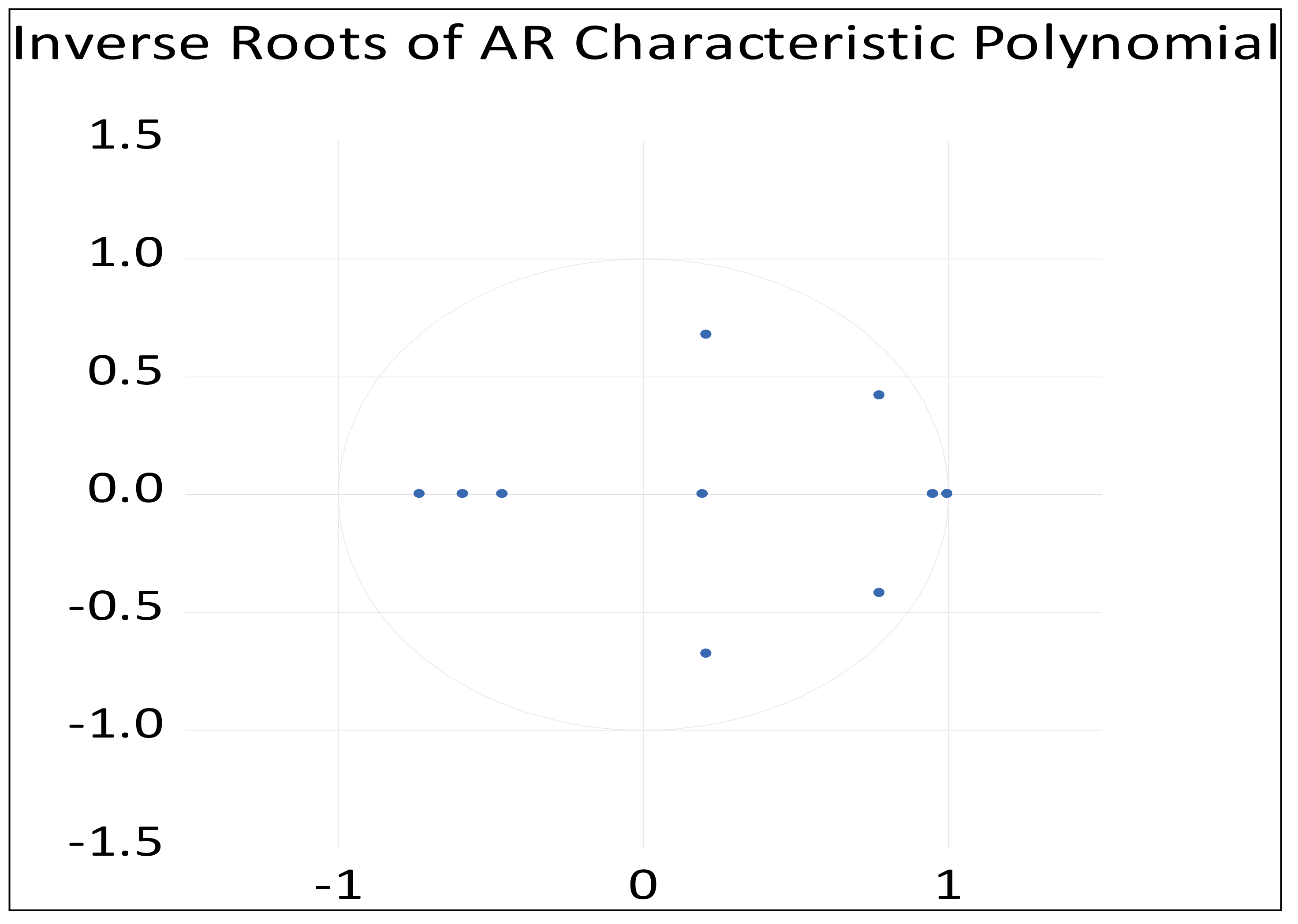
Figure 2 indicates the inverse roots of the characteristic polynomial. The roots characteristic polynomial is used to check the stability of the VECM. The vector error correction specifications impose one unit-root outside the unit circle (Eigen statistics of the respective matrix is exactly one or less); hence, the model satisfies the vector auto-regressive (VAR) stability conditions, and the VECM is acceptable in a statistical sense to make inferences.

Figure 2. Showing the stability condition of VAR.

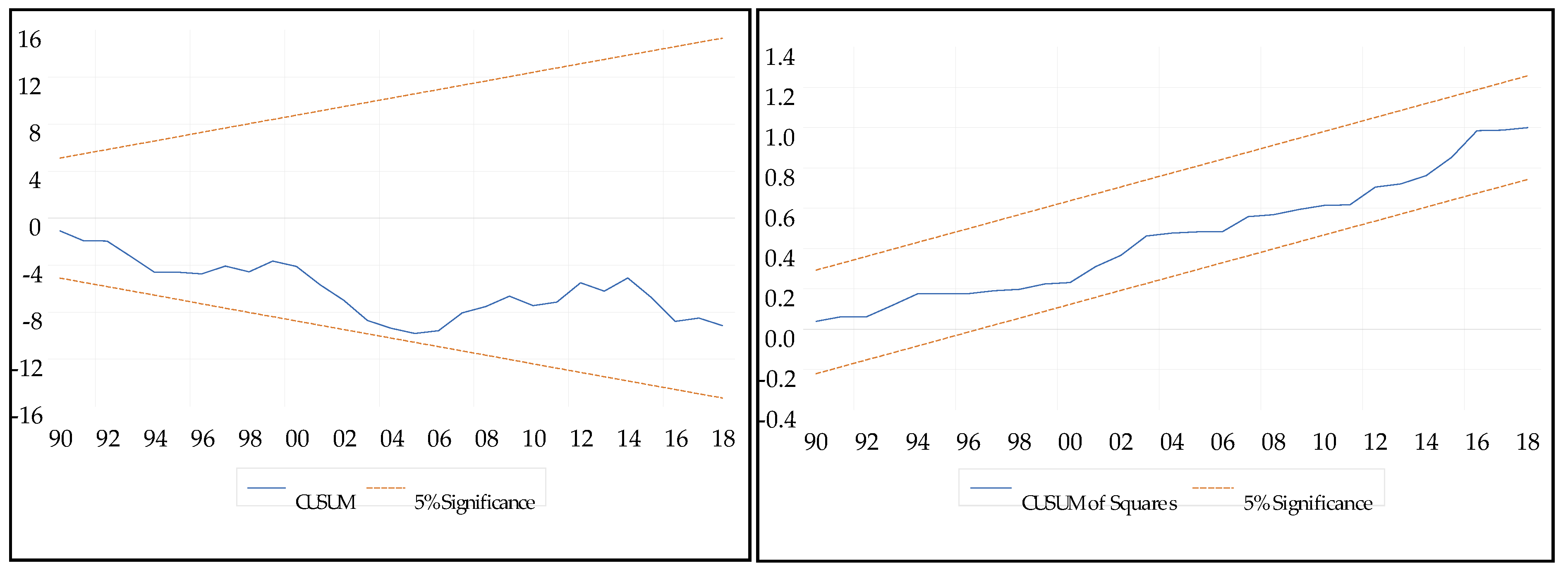
The CUSUM and CUSUMsq test for instability of parameters from the ARDL model is shown in Figure 3. The CUSUM and CUSUMsq tests are used to ascertain the parameter instability of the equation employed in the autoregressive distributed lag model. The equation parameter is stable enough to estimate the long- and short-term causalities in the ARDL model because the plots in CUSUM and CUSUMsq tests are within the critical bound at the 5% level of significance.

Figure 3. Plot of CUSUM and CUSUMsq tests for the parameter stability.

3.6. Variance Decomposition Analysis

The estimated results of the variance decomposition analysis method are presented in Table 12. The estimated results demonstrated that approximately 58.4% of the future fluctuations in LCO₂E are due to changes in LENU, 2.8% of the future fluctuations in LCO₂E are due to changes in LGDP, and 0.43% of the future fluctuations in LCO₂E are due to changes in LPG. Moreover, Table 12 indicates that approximately 3.37% of the future fluctuations in LENU are due to changes in LGDP, 9.6% of the future fluctuations in LENU are due to changes in LCO₂E, and 0.96% of the future fluctuations in LENU are due to changes in LPG. In addition, evidence from Table 12 shows that approximately 19.9% of the future fluctuations in LGDP are due to changes in LCO₂E, 4.95% of the future fluctuations in LGDP are due to changes in LENU, and 3.08% of the future fluctuations in LGDP are due to changes in LPG. Finally, the evidence from Table 12 shows that approximately 13.67% of the future fluctuations in LPG are due to changes in LCO₂E, 49.81% of the future fluctuations in LPG are due to changes in LENU, and 3.01% of the future fluctuations in LPG are due to changes in LGDP.

Table 12. Variance Decomposition of Cholesky ordering, CO₂E, ENU, GDP, PG.

Variance Decomposition of LCO2E
PERIOD	S.E.	LCO2E	LENU	LGDP	LPG
1	0.0297	100.00	0.0000	0.0000	0.0000
2	0.0399	95.1113	4.32803	0.0880	0.4725
3	0.0535	86.0290	12.0430	1.1393	0.7885
4	0.0677	76.1935	31.0071	0.9965	0.9714
5	0.0839	67.1935	31.0071	0.9965	0.8027
6	0.1008	59.7080	38.6221	1.0943	0.5754
7	0.1186	53.0662	44.9805	1.5282	0.4249
8	0.1368	47.3089	50.3303	1.9836	0.3770
9	0.1554	42.3763	54.7890	2.4390	0.3955
10	0.1741	38.2628	58.4905	2.8105	0.4360
Variance Decomposition of energy use
1	0.3361	51.13904	48.8609	0.0000	0.0000
2	0.5215	39.8865	59.9877	0.1115	0.0140
3	0.8061	30.1926	68.7380	0.9433	0.1260
4	1.0815	23.9279	74.4465	1.3556	0.2698
5	1.4095	19.2367	78.3408	1.9940	0.4283
6	1.7386	16.1486	81.0207	2.2355	0.5950
7	2.0929	13.8367	82.8151	2.6036	0.7445
8	2.4498	12.0967	84.1454	2.8963	0.8614
9	2.8206	10.7237	85.1587	3.1874	0.9301
10	3.1945	9.65864	86.0046	3.3765	0.9601
Variance Decomposition of GDP
1	1.8036	0.7467	2.5201	96.7331	0.0000
2	1.9037	1.0028	5.8013	90.2223	2.9735
3	1.9954	4.7707	5.3044	86.1778	3.7469
4	2.1137	11.6048	4.7553	80.1219	3.5183
5	2.1616	13.5756	4.9742	78.0812	3.3688
6	2.1888	14.7979	4.8545	77.0602	3.2872
7	2.2026	15.7765	4.8090	76.1603	3.2540
8	2.2256	17.4091	4.7140	74.6847	3.1920
9	2.2469	18.7530	4.8419	73.2731	3.1318
10	2.2670	19.8827	4.9584	72.0764	3.0824
Variance Decomposition of population growth
1	0.0023	0.2286	1.8278	2.6730	95.2704
2	0.0064	0.1110	5.3148	3.3273	91.2467
3	0.0121	1.6274	8.6706	4.6169	85.0849
4	0.0188	4.2747	12.9098	6.0204	76.7949
5	0.0258	7.2980	17.7646	6.5832	68.3540
6	0.0327	10.0534	23.4960	6.2863	60.1642
7	0.0390	12.1286	29.9636	5.4795	52.4280
8	0.0449	13.3712	36.8366	4.5351	45.2569
9	0.0505	13.8273	43.5946	3.6819	38.8959
10	0.0558	13.6762	49.8190	3.01609	33.4887

Authors own completion.

4. Conclusion and Policy Recommendations

The study has investigated the causal nexus between carbon dioxide emissions (CO₂E), GDP, energy use (ENU), and population growth (PG) in India over the period 1981 to 2018 by comparing VECM and ARDL models. For stationarity analysis of selected variables, we used unit root tests. The ADF and PP unit root tests showed that all the time series variables are stationarity at the first difference I(1). We applied VECM-based Granger causality to analyse the study variable for causal relationships. Furthermore, the study performed variance decomposition (VDC) analysis using the Cholesky method, stability, and diagnostic tests.

The VECM and ARDL models evidence shows that CO₂E, ENU, GDP, and PG are cointegrated. There was evidence of bi-directional causality running from ENU to GDP and a uni-directional causality running from ENU, GDP, and PG to CO₂E and PG to ENU. Evidence from joint-Granger causality shows a unidirectional causality running from CO₂E to a joint of ENU, GDP, and PG; ENU to a joint of CO₂E, GDP, and PG; GDP to a joint of CO₂E, ENU, and PG, respectively. Moreover, the long-term (LT) elasticities indicate that the 1% increase in PG in India will increase CO₂E by 1.4%, a 1% increase in GDP in India will increase CO₂E by 0.30%, and a 1% increase in ENU in India will increase CO₂E by 0.63%. There was also evidence of a short-term (ST) equilibrium association between ENU and CO₂E as well as GDP and CO₂E.

The ARDL-bound test cointegration outcomes yield evidence of a long-term equilibrium between CO₂E, ENU, GDP, and PG in India. According to the variance decomposition analysis, 58.4% of the future fluctuations in CO₂E are due to changes in ENU, 2.8% of the future fluctuations in CO₂E are due to changes in GDP, and 0.43% of the future fluctuations in CO₂E due to changes in PG. Furthermore, 3.37% of the future fluctuations in ENU are due to changes in GDP, 9.6% of the future fluctuations in ENU are due to changes in CO₂E, and 0.96% of the future fluctuations in ENU are due to changes in PG. In addition, 19.9% of the future fluctuations in GDP are due to changes in CO₂E, 4.95% of the future fluctuations in GDP are due to changes in ENU, and 3.08% of the future fluctuations in GDP are due to PG. In addition, 3.67% of the future fluctuations in PG are due to changes in CO₂E, 49.81% of the future fluctuations in PG are due to changes in ENU, and 3.01% of the future fluctuations in PG are due to changes in GDP.

Based on our study’s findings, this experimental study also proposes the following policy recommendations for the country of India: It is worth noting that India’s ENU has a long-term effect on CO₂E. India is one of the top 10 countries most severely affected by CO₂E.; hence, atmospheric threats need to be addressed seriously. Specifically, the Indian government must stimulate CO₂E reducing activities through increasing alternative energy resources such as solar, wind, geothermal sources, biodiesel fuel, and environmentally sensitive technologies that can be effectively supported. It is suggested that the Indian government teach local people in order to motivate them to plant trees with the forest department to enhance the proportion of forest in India and control environmental degradation.

Furthermore, the estimated results show that environmental degradation is the main reason for economic growth. Hence, it is advised that India’s economic growth policies be revised to address environmental degradation. To avoid CO₂ emissions, population growth, natural resources, and the ecological system must be balanced to lower CO₂ emissions. These resources might otherwise be affected by CO₂ emissions. Finally, enhancing energy effectiveness and introducing energy management options nationally by making clean energy accessible will help decrease CO₂E. To control long-term environmental degradation, policymakers are advised to follow policies that encourage the use of environmentally friendly equipment, vehicles, machinery, and utilities to reduce environmental degradation.

References

1. Danish, D.; Ozcan, B.; Ulucak, R. An empirical investigation of nuclear energy consumption and carbon dioxide (CO2) emission in India: Bridging IPAT and EKC hypotheses. Nucl. Eng. Technol. 2021, 53, 2056–2065. [Google Scholar] [CrossRef]
2. Balint, T.; Lamperti, F.; Mandel, A.; Napoletano, M.; Roventini, A.; Sapio, A. Complexity and the Economics of Climate Change: A Survey and a Look Forward. Ecol. Econ. 2017, 138, 252–265. [Google Scholar] [CrossRef] [Green Version]
3. Fouquet, R. Lessons from energy history for climate policy: Technological change, demand and economic development. Energy Res. Soc. Sci. 2016, 22, 79–93. [Google Scholar] [CrossRef] [Green Version]
4. Kasman, A.; Duman, Y.S. CO2 emissions, economic growth, energy consumption, trade and urbanization in new EU member and candidate countries: A panel data analysis. Econ. Model. 2015, 44, 97–103. [Google Scholar] [CrossRef]
5. Neog, Y.; Yadava, A.K. Nexus among CO2 emissions, remittances, and financial development: A NARDL approach for India. Environ. Sci. Pollut. Res. 2020, 27, 44470–44481. [Google Scholar] [CrossRef] [PubMed]
6. World Bank. World Development Indicators; The World Bank: Washington, DC, USA, 2019; Available online: https://elibrary.worldbank.org/doi/abs/10.1596/978-1-4648-0163-1 (accessed on 26 February 2020).
7. Global Footprint Network, 2019. Available online: https://www.footprintnetwork.org/our-work/ecological-footprint/ (accessed on 30 June 2019).
8. IQ Air. 2019 World Air Quality Report: Region & City PM2.5 Ranking. 2019. Available online: https://www.iqair.com/us/world-most-polluted-cities (accessed on 26 February 2020).
9. Global Carbon Project. 2018. Available online: https://www.globalcarbonproject.org/ (accessed on 5 December 2018).
10. Global Energy Statistical Yearbook 2020. Available online: https://yearbook.enerdata.net/ (accessed on 12 January 2021).
11. World Energy Outlook, 2014–15 Prepared by International Energy Agency (IEA). Available online: https://www.iea.org/topics/world-energy-outlook (accessed on 1 November 2014).
12. Sustainable Development Goals (2015) by United Nations. Available online: https://sustainabledevelopment.un.org/?menu=1300 (accessed on 30 December 2015).
13. Mccollum, D.L.; Echeverri, L.G.; Busch, S.; Pachauri, S.; Parkinson, S.; Rogelj, J.; Krey, V.; Minx, J.C.; Nilsson, M.; Stevance, A.-S.; et al. Connecting the sustainable development goals by their energy inter-linkages. Environ. Res. Lett. 2018, 13, 033006. [Google Scholar] [CrossRef]
14. World Economic Outlook. Prepared by International Monetary Fund. 2019. Available online: https://www.imf.org/en/Publications/WEO (accessed on 15 October 2019).
15. Bekun, F.V.; Emir, F.; Sarkodie, S.A. Another look at the relationship between energy consumption, carbon dioxide emissions, and economic growth in South Africa. Sci. Total Environ. 2019, 655, 759–765. [Google Scholar] [CrossRef] [PubMed]
16. Manigandan, P.; Alam, S.; Alharthi, M.; Khan, U.; Alagirisamy, K.; Pachiyappan, D.; Rehman, A. Forecasting Natural Gas Production and Consumption in United States-Evidence from SARIMA and SARIMAX Models. Energies 2021, 14, 6021. [Google Scholar] [CrossRef]
17. Song, Z. Economic growth and carbon emissions: Estimation of a panel threshold model for the transition process in China. J. Clean. Prod. 2021, 278, 123773. [Google Scholar] [CrossRef]
18. Grossman, G.M.; Krueger, A.B. Economic Growth and the Environment. Q. J. Econ. 1995, 110, 353–377. [Google Scholar] [CrossRef] [Green Version]
19. Ang, J.B. CO2 emissions, energy consumption, and output in France. Energy Policy 2007, 35, 4772–4778. [Google Scholar] [CrossRef]
20. Ajmi, A.N.; Inglesi-Lotz, R. Biomass energy consumption and economic growth nexus in OECD countries: A panel analysis. Renew. Energy 2020, 162, 1649–1654. [Google Scholar] [CrossRef]
21. Bouyghrissi, S.; Berjaoui, A.; Khanniba, M. The nexus between renewable energy consumption and economic growth in Morocco. Environ. Sci. Pollut. Res. 2021, 28, 5693–5703. [Google Scholar] [CrossRef] [PubMed]
22. Armeanu, D.S.; Joldes, C.C.; Gherghina, S.C.; Andrei, J.V. Understanding the multidimensional linkages among renewable energy, pollution, economic growth and urbanization in contemporary economies: Quantitative assessments across different income countries’ groups. Renew. Sustain. Energy Rev. 2021, 142, 110818. [Google Scholar] [CrossRef]
23. Boutabba, M.A. The impact of financial development, income, energy and trade on carbon emissions: Evidence from the Indian economy. Econ. Model. 2014, 40, 33–41. [Google Scholar] [CrossRef] [Green Version]
24. Komal, R.; Abbas, F. Linking financial development, economic growth and energy consumption in Pakistan. Renew. Sustain. Energy Rev. 2015, 44, 211–220. [Google Scholar] [CrossRef]
25. Nathaniel, S.P.; Alam, S.; Murshed, M.; Mahmood, H.; Ahmad, P. The roles of nuclear energy, renewable energy, and economic growth in the abatement of carbon dioxide emissions in the G7 countries. Environ. Sci. Pollut. Res. 2021, 28, 47957–47972. [Google Scholar] [CrossRef] [PubMed]
26. Sehrawat, M.; Giri, A.K.; Mohapatra, G. The impact of financial development, economic growth and energy consumption on environmental degradation: Evidence from India. Manag. Environ. Qual. Int. J. 2015, 26, 666–682. [Google Scholar] [CrossRef]
27. Khan, A.Q.; Saleem, N.; Fatima, S.T. Financial development, income inequality, and CO2 emissions in Asian countries using STIRPAT model. Environ. Sci. Pollut. Res. 2018, 25, 6308–6319. [Google Scholar] [CrossRef] [PubMed]
28. Murshed, M.; Rahman, A.; Alam, S.; Ahmad, P.; Dagar, V. The nexus between environmental regulations, economic growth, and environmental sustainability: Linking environmental patents to ecological footprint reduction in South Asia. Environ. Sci. Pollut. Res. 2021, 28, 49967–49988. [Google Scholar] [CrossRef] [PubMed]
29. Rahman, Z.U.; Cai, H.; Ahmad, M. A new look at the remittances-fdi- energy-environment nexus in the case of selected asian nations. Singap. Econ. Rev. 2019, 1–19. [Google Scholar] [CrossRef]
30. Ghosh, B.; Alam, K.J.; Osmani, A.G. Economic Growth, CO2 Emissions and Energy Consumption: The Case of Bangladesh. Int. J. Bus. Econ. Res. 2014, 3, 220. [Google Scholar] [CrossRef] [Green Version]
31. Zaidi, S.; Saidi, K. Environmental pollution, health expenditure and economic growth in the Sub-Saharan Africa countries: Panel ARDL approach. Sustain. Cities Soc. 2018, 41, 833–840. [Google Scholar] [CrossRef]
32. Adebayo, T.S.; Akinsola, G.D. Investigating the Causal Linkage Among Economic Growth, Energy Consumption and CO2 Emissions in Thailand: An Application of the Wavelet Coherence Approach. Int. J. Renew. Energy Dev. 2021, 10, 17–26. [Google Scholar] [CrossRef]
33. Ahmad, M.; Khan, Z.; Rahman, Z.U.; Khan, S. Does financial development asymmetrically affect CO2 emissions in China? An application of the nonlinear autoregressive distributed lag (NARDL) model. Carbon Manag. 2018, 9, 631–644. [Google Scholar] [CrossRef]
34. Asumadu-Sarkodie, S.; Owusu, P.A. The relationship between carbon dioxide and agriculture in Ghana: A comparison of VECM and ARDL model. Environ. Sci. Pollut. Res. 2016, 23, 10968–10982. [Google Scholar] [CrossRef]
35. Adebayo, T.S. Revisiting the EKC hypothesis in an emerging market: An application of ARDL-based bounds and wavelet coherence approaches. SN Appl. Sci. 2020, 2, 1945. [Google Scholar] [CrossRef]
36. Mirza, F.M.; Kanwal, A. Energy consumption, carbon emissions and economic growth in Pakistan: Dynamic causality analysis. Renew. Sustain. Energy Rev. 2017, 72, 1233–1240. [Google Scholar] [CrossRef]
37. Osobajo, O.; Otitoju, A.; Otitoju, M.; Oke, A. The Impact of Energy Consumption and Economic Growth on Carbon Dioxide Emissions. Sustainability 2020, 12, 7965. [Google Scholar] [CrossRef]
38. Acaravci, A.; Ozturk, I. On the relationship between energy consumption, CO2 emissions and economic growth in Europe. Energy 2010, 35, 5412–5420. [Google Scholar] [CrossRef]
39. World Bank India Data. 2021. Available online: https://data.worldbank.org/country/india (accessed on 11 January 2021).
40. Iorember, P.T.; Goshit, G.G.; Dabwor, D.T. Testing the nexus between renewable energy consumption and environmental quality in Nigeria: The role of broad-based financial development. Afr. Dev. Rev. 2020, 32, 163–175. [Google Scholar] [CrossRef]
41. Usman, O.; Akadiri, S.S.; Adeshola, I. Role of renewable energy and globalization on ecological footprint in the USA: Implications for environmental sustainability. Environ. Sci. Pollut. Res. 2020, 27, 30681–30693. [Google Scholar] [CrossRef]
42. Gul, S.; Zou, X.; Hassan, C.H.; Azam, M.; Zaman, K. Causal nexus between energy consumption and carbon dioxide emission for Malaysia using maximum entropy bootstrap approach. Environ. Sci. Pollut. Res. 2015, 22, 19773–19785. [Google Scholar] [CrossRef] [PubMed]
43. Fei, L.; Dong, S.; Xue, L.; Liang, Q.; Yang, W. Energy consumption-economic growth relationship and carbon dioxide emissions in China. Energy Policy 2011, 39, 568–574. [Google Scholar] [CrossRef]
44. Johansen, S. Likelihood-Based Inference in Cointegrated Vector Autoregressive Models OUP Catalogue; Oxford University Press: Oxford, UK, 1995. [Google Scholar]
45. Brown, R.L.; Durbin, J.; Evans, J.M. Techniques for Testing the Constancy of Regression Relationships over Time. J. R. Stat. Soc. Ser. B Stat. Methodol. 1975, 37, 149–163. [Google Scholar] [CrossRef]
46. Dickey, D.A.; Fuller, W.A. Distribution of the Estimators for Autoregressive Time Series with a Unit Root. J. Am. Stat. Assoc. 1979, 74, 427–431. [Google Scholar] [CrossRef]
47. Phillips, P.C.B.; Perron, P. Testing for a Unit Root in Time Series Regression. 1988, Volume 75. Available online: https://about.jstor.org/terms (accessed on 14 September 2011).
48. Granger, C. Some recent development in a concept of causality. J. Econ. 1988, 39, 199–211. [Google Scholar] [CrossRef]
49. Wang, X. Determinants of ecological and carbon footprints to assess the framework of environmental sustainability in BRICS countries: A panel ARDL and causality estimation model. Environ. Res. 2021, 197, 111111. [Google Scholar] [CrossRef] [PubMed]
50. Pradhan, R.P.; Norman, N.R.; Badir, Y.; Samadhan, B. Transport Infrastructure, Foreign Direct Investment and Economic Growth Interactions in India: The ARDL Bounds Testing Approach. Procedia -Soc. Behav. Sci. 2013, 104, 914–921. [Google Scholar] [CrossRef] [Green Version]
51. Rehman, A.; Ma, H.; Radulescu, M.; Sinisi, C.I.; Paunescu, L.M.; Alam, M.S.; Alvarado, R. The Energy Mix Dilemma and Environmental Sustainability: Interaction among Greenhouse Gas Emissions, Nuclear Energy, Urban Agglomeration, and Economic Growth. Energies 2021, 14, 7703. [Google Scholar] [CrossRef]
52. Hamid, I.; Alam, M.S.; Murshed, M.; Jena, P.K.; Sha, N.; Alam, M.N. The roles of foreign direct investments, economic growth, and capital investments in decarbonizing the economy of Oman. Environ. Sci. Pollut. Res. 2021, 15, 1–7. [Google Scholar] [CrossRef] [PubMed]
53. Jarque, C.M.; Bera, A.K. Efficient tests for normality, homoscedasticity and serial independence of regression residuals. Econ. Lett. 1980, 6, 255–259. [Google Scholar] [CrossRef]