
The Influence of Investors’ Mood on the Stock Prices: Evidence from Energy Firms in Warsaw Stock Exchange, Poland


Abstract
:1. Introduction
2. Emotions–Weather–Market
3. Materials and Methods
4. Results
5. Discussion and Conclusions
- not all analytical methods are equally effective. This can be clearly seen in the example of the VAR analysis. The number of positive indications obtained in this case significantly exceeds the relevance of weather factors in the OLS modeling. The limitations of the OLS methodology are described earlier;
- co-integration analysis with the use of the Engle–Granger and Johansen tests is in a sense unjustified as it always indicates relationships between variables. It, therefore, disrupts the general view of causal relationships;
- determining the direction of the relationship weather factor → rate of return may be based only on the values of the tangent of the angle of inclination in the regression analysis;
- the most common determinants of the rate of return and the volume of trading include the weather factor in the form of average daily relative humidity and average wind speed. The first of these weather variables is the cause of the percentage changes in stock prices, the second is responsible for changes in the trading volume. The results in this case are different from those obtained in the studies of the team of Tarczyński et al. [54] with the use of ARCH class models. Then, the variable with a clear influence was atmospheric pressure. Therefore, it can be assumed that the considered causality depends on the methodology used;
- the trading volume seems to be much more susceptible to possible influences from independent variables;
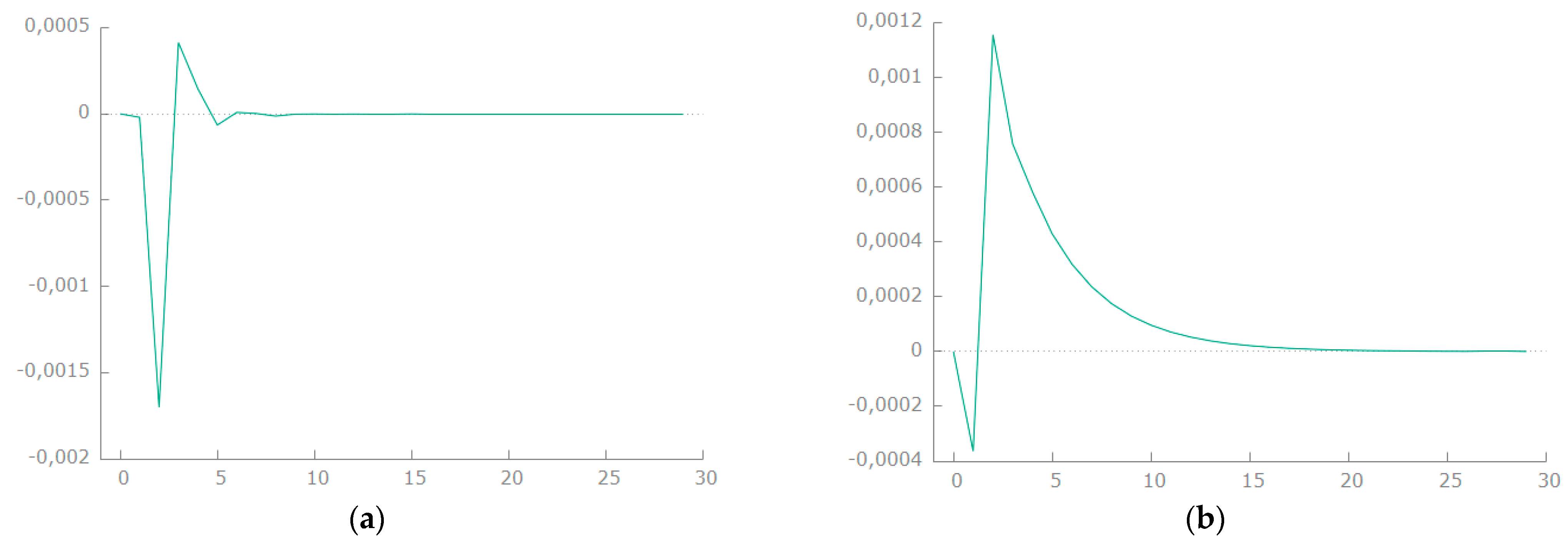
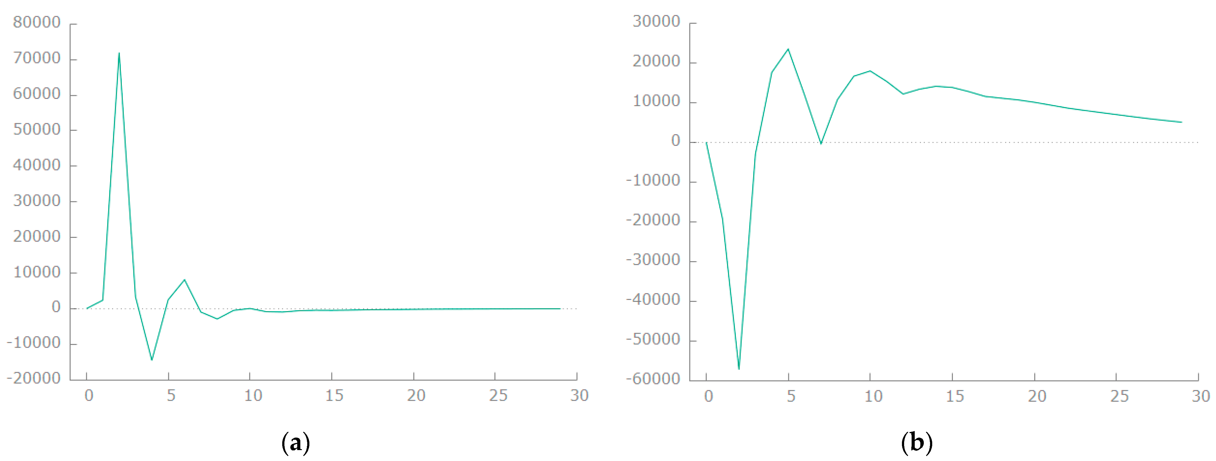
- impulse response functions turn out to be extremely useful in VAR analyses, allowing additional inference in the case of dependence from meteorological time series;
- it would be advisable to continue research in the causality area and to verify the effectiveness of indications in the context of the distribution of the analyzed variables. Perhaps the nature of the distribution itself (convergence or divergence with the normal distribution) may affect the final indications;
- in the case of some weather variables, consideration should also be given to take into account the phenomenon of seasonality over a longer period of time;
- in general, it can be said that the indications depend on the type of method used and the nature of the test itself. Hence, weather variables play a role in modeling the mood of stock market investors investing in the energy sector, mainly in the context of Granger causality analysis.
- many studies of this type do not take into account the phenomenon of the seasonality of twists. This may cause a distortion of the causal relationships between investor behavior and meteorological factors;
- some analyses did not investigate whether variables take into account other weather indicators. For instance, the effect of a certain temperature level on mood may depend on whether or not it is raining;
- as a rule, this type of analysis does not take into account the behavior of investors at different times of the year. There may be a dependence that higher winter/summer temperatures may positively/negatively affect decision-making processes;
Author Contributions
Funding
Institutional Review Board Statement
Informed Consent Statement
Data Availability Statement
Acknowledgments
Conflicts of Interest
References
- Mehra, R.; Prescott, E.C. The equity premium: A puzzle. J. Monet. Econ. 1985, 15, 145–161. [Google Scholar] [CrossRef]
- Kahneman, D.; Knetsch, J.L.; Thaler, R. Fairness as a constraint on profit seeking: Entitlements in the market. Am. Econ. Rev. 1986, 76, 728–741. [Google Scholar] [CrossRef]
- Allen, M.A.; Fischer, G.J. Ambient Temperature Effects on Paired Associate Learning? Ergonomics 1978, 21, 95–101. [Google Scholar] [CrossRef]
- Hu, T.-Y.; Xie, X.; Li, J. Negative or positive? The effect of emotion and mood on risky driving. Transp. Res. Part F Traffic Psychol. Behav. 2013, 16, 29–40. [Google Scholar] [CrossRef]
- Keller, M.C.; Fredrickson, B.L.; Ybarra, O.; Cote, S.; Johnson, K.; Mikels, J.; Conway, A.; Wager, T. A Warm Heart and a Clear Head: The Contingent Effects of Weather on Mood and Cognition. Psychol. Sci. 2005, 16, 724–731. [Google Scholar] [CrossRef]
- Howarth, E.; Hoffman, M.S. A multidimensional approach to the relationship between mood and weather. Br. J. Psychol. 1984, 75, 15–23. [Google Scholar] [CrossRef] [PubMed]
- Loewenstein, G. Emotions in Economic Theory and Economic Behavior. Am. Econ. Rev. 2000, 90, 426–432. [Google Scholar] [CrossRef] [Green Version]
- Saunders, E.M. Stock prices and the Wall Street weather. Am. Econ. Rev. 1993, 83, 1337–1345. [Google Scholar]
- Hirshleifer, D.; Shumway, T. Good Day Sunshine: Stock Returns and the Weather. J. Financ. 2003, 58, 1009–1032. [Google Scholar] [CrossRef]
- Floros, C. Stock market returns and the temperature effect: New evidence from Europe. Appl. Financ. Econ. Lett. 2008, 4, 461–467. [Google Scholar] [CrossRef]
- Shim, H.; Kim, H.; Kim, J.; Ryu, D. Weather and stock market volatility: The case of a leading emerging market. Appl. Econ. Lett. 2014, 22, 987–992. [Google Scholar] [CrossRef]
- Pardo, A.; Valor, E. Spanish stock returns: Where is the weather effect? Eur. Financ. Manag. 2003, 9, 117–126. [Google Scholar] [CrossRef]
- Cao, M.; Wei, J. Stock market returns: A note on temperature anomaly. J. Bank. Financ. 2005, 29, 1559–1573. [Google Scholar] [CrossRef]
- Chang, T.; Nieh, C.-C.; Yang, M.J.; Yang, T.-Y. Are stock market returns related to the weather effects? Empirical evidence from Taiwan. Phys. A Stat. Mech. Appl. 2005, 364, 343–354. [Google Scholar] [CrossRef]
- Dowling, M.; Lucey, B.M. Robust global mood influences in equity pricing. J. Multinatl. Financ. Manag. 2008, 18, 145–164. [Google Scholar] [CrossRef]
- Wright, W.F.; Bower, G.H. Mood effects on subjective probability assessment. Organ. Behav. Hum. Decis. Process. 1992, 52, 276–291. [Google Scholar] [CrossRef]
- Bagozzi, R.P.; Gopinath, M.; Nyer, P.U. The Role of Emotions in Marketing. J. Acad. Mark. Sci. 1999, 27, 184–206. [Google Scholar] [CrossRef]
- Isen, A.M.; Shalker, T.E.; Clark, M.; Karp, L. Affect, accessibility of material in memory, and behavior: A cognitive loop? J. Pers. Soc. Psychol. 1978, 36, 1–12. [Google Scholar] [CrossRef]
- Forgas, J.P.; Bower, G.H. Mood effects on person-perception judgments. J. Personal. Soc. Psychol. 1987, 53, 53–60. [Google Scholar] [CrossRef]
- Clore, G.L.; Schwarz, N.; Conway, M. Affective causes and consequences of social information processing. In Handbook of Social Cognition: Basic Processes; Applications; Wyer, W.R.S., Srull, T.K., Eds.; Lawrence Erlbaum Associates, Inc.: Hillsdale, NJ, USA, 1994; pp. 323–417. [Google Scholar]
- Forgas, J.P. Mood and judgment: The affect infusion model (AIM). Psychol. Bull. 1995, 117, 39–66. [Google Scholar] [CrossRef]
- Bless, H.; Schwarz, N.; Kemmelmeier, M. Mood and Stereotyping: Affective States and the Use of General Knowledge Structures. Eur. Rev. Soc. Psychol. 1996, 7, 63–93. [Google Scholar] [CrossRef]
- Isen, A. Positive affect and decision making. In Handbook of Emotions; Lewis, W.M., Haviland-Jones, J., Eds.; The Guilford Press: New York, NY, USA, 2000; pp. 261–277. [Google Scholar]
- Schwarz, N. Feelings as information: Informational and motivational functions of affective states. In Handbook of Motivation and Cognition; Sorrentino, W.R., Higgins, E.T., Eds.; Guildford Press: New York, NY, USA, 1990; Volume 2, pp. 527–561. [Google Scholar]
- Petty, R.E.; Gleicher, F.; Baker, S.M. Multiple roles for affect in persuasion. In International Series in Experimental Social Psychology. Emotion and Social Judgments; Forgas, W.J.P., Ed.; Pergamon Press: Oxford, UK, 1991; pp. 181–200. [Google Scholar]
- Sinclair, R.C.; Mark, M.M. The effects of mood state on judgemental accuracy: Processing strategy as a mechanism. Cogn. Emot. 1995, 9, 417–438. [Google Scholar] [CrossRef]
- Bless, H.; Clore, G.L.; Schwarz, N.; Golisano, V.; Rabe, C.; Wolk, M. Mood and the use of scripts: Does being in a happy mood really lead to mindlessness? J. Personal. Soc. Psychol. 1996, 71, 665–679. [Google Scholar] [CrossRef]
- Johnson, E.J.; Tversky, A. Affect, generalization, and the perception of risk. J. Personal. Soc. Psychol. 1983, 45, 20–31. [Google Scholar] [CrossRef]
- Arkes, H.R.; Herren, L.T.; Isen, A.M. The role of potential loss in the influence of affect on risk-taking behavior. Organ. Behav. Hum. Decis. Process. 1988, 42, 181–193. [Google Scholar] [CrossRef]
- Loewenstein, G.F.; Weber, E.U.; Hsee, C.K.; Welch, N. Risk as feelings. Psychol. Bull. 2001, 127, 267–286. [Google Scholar] [CrossRef]
- Slovic, P.; Finucane, M.L.; Peters, E.; MacGregor, D.G. The affect heuristic. Eur. J. Oper. Res. 2007, 177, 1333–1352. [Google Scholar] [CrossRef]
- Frijda, N.H. The laws of emotion. Am. Psychol. 1988, 43, 349–358. [Google Scholar] [CrossRef]
- Wilson, T.D.; Schooler, J.W. Thinking too much: Introspection can reduce the quality of preferences and decisions. J. Pers. Soc. Psychol. 1991, 60, 181–192. [Google Scholar] [CrossRef]
- Schwarz, N.; Clore, G.L. Mood, misattribution, and judgments of well-being: Informative and directive functions of affective states. J. Pers. Soc. Psychol. 1983, 45, 513–523. [Google Scholar] [CrossRef]
- Loughran, T.; Schultz, P. Weather, Stock Returns, and the Impact of Localized Trading Behaviour. J. Financ. Quant. Anal. 2004, 39, 343–364. [Google Scholar] [CrossRef] [Green Version]
- Kamstra, M.J.; Kramer, L.A.; Levi, M.D. Losing sleep at the market: The daylight saving anomaly. Am. Econ. Rev. 2000, 90, 1005–1011. [Google Scholar] [CrossRef] [Green Version]
- Kang, S.H.; Jiang, Z.; Yoon, S.M. Weather Effects on the Returns and Volatility of Hong Kong and Shenzhen Stock Markets. 2010. Available online: http://citeseerx.ist.psu.edu/viewdoc/download?doi=10.1.1.466.5379&rep=rep1&type=pdf (accessed on 14 August 2021).
- Dowling, M.; Brian, M.L. Weather, Biorhythms, Beliefs and Stock Returns Some—Preliminary Irish Evidence. Int. Rev. Financ. Anal. 2005, 14, 337–355. [Google Scholar] [CrossRef]
- Symeonidis, L.; Daskalakis, G.; Markellos, R.N. Does the weather affect stock market volatility? Financ. Res. Lett. 2010, 7, 214–223. [Google Scholar] [CrossRef] [Green Version]
- Goetzmann, W.N.; Zhu, N. Rain or Shine: Where is the Weather Effect? Eur. Financ. Manag. 2005, 11, 559–578. [Google Scholar] [CrossRef]
- Hong, H.; Kubik, J.D.; Stein, J.C. Social Interaction and Stock-Market Participation. J. Financ. 2004, 59, 137–163. [Google Scholar] [CrossRef] [Green Version]
- Vlady, S.; Tufan, E.; Hamarat, B. Causality of Weather Conditions in Australian Stock Equity Returns. Rev. Tinerilor Econ. 2011, 1, 187–194. [Google Scholar]
- Worthington, A. An Empirical Note on Weather Effects in the Australian Stock Market. Econ. Pap. A J. Appl. Econ. Policy 2009, 28, 148–154. [Google Scholar] [CrossRef]
- Keef, S.P.; Roush, M.L. Daily weather effects on the returns of Australian stock indices. Appl. Financ. Econ. 2007, 17, 173–184. [Google Scholar] [CrossRef]
- Wang, Y.-H.; Lin, C.-T.; Lin, J.D. Does weather impact the stock market? Empirical evidence in Taiwan. Qual. Quant. 2011, 46, 695–703. [Google Scholar] [CrossRef]
- Tuna, G. Analyzıng Weather Effect on Istanbul Stock Exchange: An Empırıcal Analysıs for 1987–2006 Period. Econ. Financ. Rev. 2014, 3, 17–25. [Google Scholar]
- Silva, P.; Almeida, L. Weather and Stock Markets: Empirical Evidence from Portugal; MPRA Paper 54119; University Library of Munich: Munich, Germany, 2011. [Google Scholar]
- Zadorozhna, O. Does Weather Affect Stock Returns Across Emergıng Markets? Master’s Thesis, Kyiv School of Economics, Kyiv, Ukraine, 2009. [Google Scholar]
- Engle, R.F.; Granger, C.W.J. Co-Integration and Error Correction: Representation, Estimation, and Testing. Econometrica 1987, 55, 251. [Google Scholar] [CrossRef]
- Johansen, S. Statistical analysis of cointegration vectors. J. Econ. Dyn. Control. 1988, 12, 231–254. [Google Scholar] [CrossRef]
- Maddala, G.S. Ekonometria; PWN: Warszawa, Poland, 2006. [Google Scholar]
- Hamulczuk, M.; Grudkowska, S.; Gędek, S.; Klimkowski, C.; Stańko, S. Essential Econometric Methods of Forecasting Agricultural Commodity Prices; Institute of Agricultural and Food Economics—National Research Institute: Warszawa, Poland, 2013. [Google Scholar]
- Kusideł, E. Dane Panelowe i Modelowanie Wielowymiarowe w Badaniach Ekonomicznych; Absolwent: Łódź, Poland, 2000. [Google Scholar]
- Tarczyński, W.; Majewski, S.; Tarczyńska-Łuniewska, M.; Majewska, A.; Mentel, G. The Impact of Weather Factors on Quotations of Energy Sector Companies on Warsaw Stock Exchange. Energies 2021, 14, 1536. [Google Scholar] [CrossRef]
- Chang, S.-C.; Chen, S.-S.; Chou, R.; Lin, Y.-H. Weather and intraday patterns in stock returns and trading activity. J. Bank. Financ. 2008, 32, 1754–1766. [Google Scholar] [CrossRef]
- Akhtari, M. Reassessment of the Weather Effect: Stock Prices and Wall Street Weather. Undergrad. Econ. Rev. 2011, 7, 1–25. [Google Scholar]
- Trombley, M.A. Stock Prices and Wall Street Weather: Additional Evidence. Q. J. Bus. Econ. 1997, 36, 11–21. [Google Scholar]
- Lee, Y.-M.; Wang, K.-M. The effectiveness of the sunshine effect in Taiwan’s stock market before and after the 1997 financial crisis. Econ. Model. 2011, 28, 710–727. [Google Scholar] [CrossRef]
- Krämer, W.; Runde, R. Stocks and the Weather: An Exercise in Data Mining or Yet Another Capital Market Anomaly? Empir. Econ. 1997, 22, 637–641. [Google Scholar] [CrossRef]
- Levy, O.; Galili, I. Stock purchase and the weather: Individual differences. J. Econ. Behav. Organ. 2008, 67, 755–767. [Google Scholar] [CrossRef]
- Shu, H.-C. Investor mood and financial markets. J. Econ. Behav. Organ. 2010, 76, 267–282. [Google Scholar] [CrossRef]

| Author (Authors) | Conclusions |
|---|---|
| Howarth, E. and Hoffman, M.S [6] | They verified the impact of eight weather variables on ten mood measures. As a result of the research, they indicated that meteorological factors such as humidity, temperature and sunshine have a significant influence on the mood. In their opinion, the duration of sunlight was associated with higher scores in terms of optimism, while high levels of humidity with lower scores in terms of concentration, and a possible increase in temperature with lower scores in terms of anxiety and skepticism. |
| Loughran, T. and Schultz, P. [35] | They showed that cloudy days have little effect on a company’s trading volume apart from extreme weather conditions, which can be attributed to other factors that may be unrelated to mood. |
| Saunders, E.M. [8] | He was the first to investigate the relationship between New York City weather and returns on the New York Stock Exchange (NYSE). As a result of the analyses, he drew the attention of economists to the possible impact of weather changes on the returns on the stock exchange. It showed a significant correlation between cloud cover and percentage changes in stock prices. |
| Kamstra, M.J., Kramer, L.A., and Levi, M.D. [36] | In their opinion, in autumn and winter, market profits are on average lower than in spring and summer. They characterized it as the beginning of a seasonal affective disorder, i.e., a depression associated with a decline in daylight. This phenomenon is particularly strong in the Scandinavian countries. According to them, due to the lack of sun, people become more depressed, which lowers the general good mood and the willingness to invest. If investors had realized this sooner, they could have prevented irrational decisions. |
| Keller, M.C., Fredrickson, B.L., Ybarra, O., Côté, S., Johnson, K., Mikels, J., Conway, A., Wager, T. [5] | They found that a pleasant temperature and atmospheric pressure are associated with better mood. Trading activity correlates strongly with the skills, personalities and moods of traders. |
| Hirshleifer, D. and Shumway, T. [9] | They investigated whether the sun can lead to a good mood, which would additionally translate into positive plot twists. In their research, they proved that there was a significant positive correlation between insolation and the rates of return. They found that investors could benefit from knowledge about their mood at any given time. Thanks to this, they can avoid mistakes caused by an unsuitable mood. |
| Kang, S.H., Jiang, Z., Lee, Y. and Yoon, S.M. [37] | They proved that weather conditions had an impact on type A funds and not on type B funds. In the period after market opening, only type B funds are heavily influenced by weather conditions, while in the profitability of both type A and type B funds, the weather has led to volatility; Shanghai Stock Exchange, 1996–2007. |
| Dowling, M. and Brian, M.L. [38] | A positive correlation was found between the results of the moisture analysis and the performance indicators in relation to slightly different opinions in this regard in the literature. The authors found the reasons for this different result of the analysis in the unusual weather conditions prevailing in Ireland; Irish Stock Exchange; 1988–2001. |
| Symeonidis, L., Daskalakis, G. and Markellos, R.N. [39] | According to the authors, cloudy days and extending and reducing night hours have a negative impact on the volatility of the stock markets. They state that the performance of the S&P index tends to have a negative effect on cloudy days; 26 international exchanges, 1982–1997. |
| Goetzman, W.N. and Zhu, N. [40] | On rainy days, market participants tend to finish trading earlier, according to the team. They note the effect of cloudy days on both liquidity and volatility; 2005. |
| Loughran, T. I Schultz, P. [35] | They addressed the issue of low volume. They saw the reasons for this condition in the difficulties in getting to work on days with snowstorms; 2004. |
| Hong, H., Kubik, J. and Stein, J. [41] | They argued that investors are more sociable and open to communication with each other on sunny days, which may explain the high volatility currently observed in the stock market; 2004 |
| Vlady, S., Tufan, E. and Hamarat, B. [42] | They showed that there was a significant change in profitability on the Australian Stock Exchange on rainy days; Australia 1992–2006. |
| Kang, S.H., Jiang, Z. and Yoon, S.M. [37] | They stated that the Hong Kong Stock Exchange was not vulnerable to extreme weather conditions; Hong Kong Stock Exchange 1999–2008. |
| Worthington, A. [43] | He examined the effects of meteorological conditions such as evaporation, relative humidity, high and low temperatures, hours of sunshine, and the direction and speed of a severe storm on the Australian stock price index and found no impact on market earnings; 1958–2005. |
| Keef, S.P. and Roush, M.L. [44] | They observed that off-season temperatures had a stronger and negative impact on stocks compared to normal temperature parameters. On the other hand, the speed of the storm and the number of cloudy days did not have such an effect; 1992–2003 |
| Floros, C. [10] | The impact of daily temperatures on the stock markets in Austria, Belgium, France, Greece and the UK was studied at different times and a negative correlation was identified between daily temperature parameters and the yields of the stock markets in Austria, Belgium and France. In turn, in the case of Greece and the UK, this correlation was positive but not statistically strong. In another study, Floros (2011) showed that weather conditions had a negative impact on market profitability, using data from the Lisbon Stock Exchange (PSI-20) in 1995–2007. The researcher also found that safety indicators were positive in January, mainly due to the low temperatures, which lead to aggressive risk taking; Austria, Belgium, France, Greece and UK Equity Markets, 2008. |
| Chang, T., Nieh, C.C., Yang, M.J. and Yang, T.Y. [14] | They examined the effect of weather conditions on earnings, against factors such as temperature, humidity and cloudy days. According to the research results, the following had a significant influence in this case: temperature and cloudy days; Taiwan Stock Exchange, July–October 2006. |
| Wang, Y., Lin, C.T. and Lin, J.D. [45] | They did not identify the impact of rainy days on market profits but showed that sunny days and temperature had a significant impact; Taiwan Stock Exchange, 2001–2007. |
| Tuna, G. [46] | He examined the effect of humidity and cloudy days on the profitability of the Istanbul Stock Index and found no effect; Istanbul Stock Exchange, 1987–2006. |
| Silva, P. and Almeida, L. [47] | Thanks to their analysis, a correlation between low temperature and high efficiency was identified; Portuguese Stock Exchange, 2000–2009. |
| Zadorozhna, O. [48] | Correlations between profitability indices, individual safety indices, commercial value, and weather conditions (storm, cloudy days, pressure, rain and humidity) at different times were examined. While correlations were identified in some countries, they were found to be low; 13 countries of Central and Eastern Europe, 2009 |
| Instrument | ADF Test | KPSS Test | ||||
|---|---|---|---|---|---|---|
| Delay | Test Statistic | p | Autocorrelation of First-Order Residuals | Test Statistic | Critical Value α = 5% and α = 1% | |
| Będzin | ||||||
| rate of return | 0 | −45.1744 | 0.0001 | −0.015 | 0.267245 | 0.462/0.743 |
| trading volume | 0 | −26.9194 | 1.220 × 10−44 | −0.048 | 1.551350 | |
| Enea | ||||||
| rate of return | 0 | −35.7359 | 1.209 × 10⁻²⁴ | 0.001 | 0.033697 | 0.462/0.743 |
| trading volume | 0 | −29.3397 | 4.378 × 10−41 | −0.047 | 1.593400 | |
| Energa | ||||||
| rate of return | 0 | −38.5467 | 4.595 × 10⁻¹⁶ | 0.000 | 0.167231 | 0.462/0.743 |
| trading volume | 0 | −24.3335 | 2.797 × 10−46 | −0.077 | 15.80410 | |
| Kogeneracja | ||||||
| rate of return | 0 | −43.3854 | 0.0001 | 0.000 | 0.244913 | 0.462/0.743 |
| trading volume | 0 | −32.4472 | 4.448 × 10−46 | −0.014 | 0.622624 | |
| ML System | ||||||
| rate of return | 0 | −23.4542 | 1.643 × 10−39 | 0.008 | 0.227393 | 0.462/0.743 |
| trading volume | 0 | −11.0043 | 5.512 × 10⁻²¹ | −0.132 | 17.56750 | |
| PGE | ||||||
| rate of return | 0 | −35.2625 | 4.451 × 10⁻²⁶ | 0.000 | 0.033137 | 0.462/0.743 |
| trading volume | 0 | −32.7535 | 2.832 × 10⁻³³ | −0.020 | 0.711201 | |
| Polenergia | ||||||
| rate of return | 0 | −37.1847 | 3.350 × 10⁻²⁰ | 0.002 | 0.512327 | 0.462/0.743 |
| trading volume | 0 | −32.4881 | 5.693 × 10⁻³⁴ | −0.017 | 0.564129 | |
| Tauron | ||||||
| rate of return | 0 | −34.277 | 5.311 × 10⁻²⁹ | 0.002 | 0.197904 | 0.462/0.743 |
| trading volume | 0 | −22.4762 | 5.342 × 10−46 | −0.066 | 6.307180 | |
| ZE PAK | ||||||
| rate of return | 0 | −39.7838 | 1.823 × 10⁻¹² | 0.000 | 0.220253 | 0.462/0.743 |
| trading volume | 0 | −31.2886 | 5.690 × 10−37 | −0.020 | 1.216120 | |
| Instrument | ADF Test | KPSS Test | ||||
|---|---|---|---|---|---|---|
| Delay | Test Statistic | p | Autocorrelation of First-Order Residuals | Test Statistic | Critical Value α = 5% and α = 1% | |
| Gdańsk | ||||||
| average daily temperature | 0 | −6.65853 | 3.412 × 10−09 | −0.072 | 1.770400 | 0.462/0.743 |
| 4 | −4.07270 | 0.001076 | −0.005 | 0.383428 | ||
| daily sum of precipitation | 0 | −34.7505 | 1.292 × 10⁻²⁷ | −0.003 | 0.163824 | |
| insolation | 0 | −19.4848 | 5.023 × 10−43 | −0.153 | 0.640190 | |
| 1 | −13.3531 | 4.477 × 10⁻³⁰ | −0.030 | 0.401188 | ||
| duration of rainfall | 0 | −29.8175 | 3.587 × 10−40 | −0.013 | 0.224766 | |
| mean daily overall cloudiness | 0 | −21.8798 | 1.193 × 10−45 | −0.030 | 0.328337 | |
| average daily wind speed | 0 | −25.6320 | 9.492 × 10−46 | −0.008 | 0.175068 | |
| average daily relative humidity | 0 | −19.9723 | 1.030 × 10−43 | −0.080 | 1.547060 | |
| 6 | −8.10506 | 2.454 × 10⁻¹⁸ | −0.003 | 0.428725 | ||
| mean daily sea level pressure | 0 | −36.5630 | 4.060 × 10⁻²² | −0.001 | 0.082570 | |
| Katowice | ||||||
| average daily temperature | 0 | −7.13979 | 1.901 × 10⁻¹⁰ | −0.014 | 1.205010 | 0.462/0.743 |
| 2 | −5.85133 | 2.707 × 10−07 | −0.019 | 0.426140 | ||
| daily sum of precipitation | 0 | −29.7677 | 2.896 × 10−40 | 0.011 | 0.251548 | |
| insolation | 0 | −21.4800 | 2.414 × 10−45 | −0.090 | 0.562847 | |
| 1 | −15.8271 | 1.435 × 10−37 | −0.027 | 0.368371 | ||
| duration of rainfall | 0 | −29.1066 | 1.678 × 10−41 | −0.011 | 0.124021 | |
| mean daily overall cloudiness | 0 | −23.4955 | 2.661 × 10−46 | −0.001 | 0.395364 | |
| average daily wind speed | 0 | −23.9630 | 2.561 × 10−46 | −0.033 | 0.334759 | |
| average daily relative humidity | 0 | −18.0161 | 1.659 × 10−40 | −0.091 | 0.953594 | |
| 2 | −11.5877 | 2.313 × 10⁻²⁴ | −0.016 | 0.436156 | ||
| mean daily sea level pressure | 0 | −37.7039 | 1.303 × 10⁻¹⁸ | −0.000 | 0.058875 | |
| Koło | ||||||
| average daily temperature | 0 | −8.67207 | 9.310 × 10⁻¹⁵ | −0.072 | 1.414050 | 0.462/0.743 |
| 3 | −5.65398 | 7.779 × 10−07 | −0.013 | 0.394922 | ||
| daily sum of precipitation | 0 | −34.2158 | 3.527 × 10⁻²⁹ | −0.010 | 0.382024 | |
| insolation | 0 | −19.3793 | 7.278 × 10−43 | −0.111 | 1.743280 | |
| 6 | −6.88035 | 6.935 × 10⁻¹⁰ | −0.007 | 0.439224 | ||
| duration of rainfall * | - | - | - | - | - | |
| mean daily overall cloudiness * | - | - | - | - | - | |
| average daily wind speed | 0 | −24.3227 | 2.808 × 10−46 | 0.004 | 2.583170 | |
| average daily relative humidity | 0 | −20.5403 | 2.046 × 10−44 | −0.088 | 0.723716 | |
| 2 | −13.4426 | 2.324 × 10⁻³⁰ | −0.006 | 0.360950 | ||
| mean daily sea level pressure | 0 | −24.4785 | 3.020 × 10−46 | 0.018 | 0.237739 | |
| Poznań | ||||||
| average daily temperature | 0 | −6.65828 | 3.418 × 10−09 | −0.072 | 1.768160 | 0.462/0.743 |
| 4 | −4.07820 | 0.001053 | −0.005 | 0.382957 | ||
| daily sum of precipitation | 0 | −34.7403 | 1.222 × 10⁻²⁷ | −0.003 | 0.163108 | |
| insolation | 0 | −19.4890 | 4.976 × 10−43 | −0.153 | 0.637882 | |
| 1 | −13.3568 | 4.357 × 10⁻³⁰ | −0.031 | 0.399831 | ||
| duration of rainfall | 0 | −30.5269 | 1.066 × 10−38 | −0.010 | 0.264330 | |
| mean daily overall cloudiness | 0 | −23.0241 | 3.292 × 10−46 | −0.023 | 0.436696 | |
| average daily wind speed | 0 | −25.5923 | 9.047 × 10−46 | −0.008 | 0.174762 | |
| average daily relative humidity | 0 | −19.9831 | 1.002 × 10−43 | −0.080 | 1.534470 | |
| 6 | −8.11923 | 2.229 × 10⁻¹³ | −0.003 | 0.425760 | ||
| mean daily sea level pressure | 0 | −36.5527 | 3.827 × 10⁻²² | −0.001 | 0.082906 | |
| Rzeszów | ||||||
| average daily temperature | 0 | −4.90820 | 3.714 × 10−05 | −0.086 | 2.201240 | 0.462/0.743 |
| 5 | −2.44556 | 0.1293 | −0.003 | 0.410210 | ||
| daily sum of precipitation | 0 | −20.6487 | 1.856 × 10−39 | 0.006 | 0.367610 | |
| insolation * | - | - | - | - | - | |
| duration of rainfall | 0 | −19.7419 | 7.614 × 10−39 | −0.001 | 0.484120 | |
| 1 | −19.7419 | 7.614 × 10−39 | −0.001 | 0.393551 | ||
| mean daily overall cloudiness | 0 | −13.9563 | 6.826 × 10⁻²⁹ | 0.005 | 0.465584 | |
| 1 | −13.9563 | 6.826 × 10⁻²⁹ | 0.005 | 0.305371 | ||
| average daily wind speed | 0 | −13.9629 | 6.574 × 10⁻²⁹ | −0.026 | 0.793649 | |
| 2 | −13.9629 | 6.574 × 10⁻²⁹ | −0.026 | 0.416820 | ||
| average daily relative humidity | 0 | −10.5698 | 9.411 × 10⁻²⁰ | −0.057 | 1.241470 | |
| 3 | −6.3716 | 1.453 × 10−08 | −0.010 | 0.442910 | ||
| mean daily sea level pressure | 0 | −10.5538 | 1.045 × 10⁻¹⁹ | 0.123 | 0.253807 | |
| Warszawa | ||||||
| average daily temperature | 0 | −6.76346 | 1.839 × 10−09 | −0.011 | 1.511100 | 0.462/0.743 |
| 3 | −4.81845 | 4.731 × 10−05 | −0.011 | 0.405907 | ||
| daily sum of precipitation | 0 | −32.9775 | 1.137 × 10⁻³² | −0.015 | 0.181474 | |
| insolation | 0 | −19.1301 | 1.774 × 10−42 | −0.108 | 1.491150 | |
| 5 | −8.64524 | 5.879 × 10⁻¹⁵ | −0.003 | 0.422109 | ||
| duration of rainfall | 0 | −28.8845 | 6.807 × 10−42 | −0.031 | 0.364404 | |
| mean daily overall cloudiness | 0 | −21.0338 | 6.075 × 10−45 | −0.042 | 0.449521 | |
| average daily wind speed | 0 | −26.2856 | 2.938 × 10−45 | 0.016 | 0.207873 | |
| average daily relative humidity | 0 | −15.1308 | 7.267 × 10⁻³⁴ | −0.096 | 0.971395 | |
| 2 | −12.3351 | 8.475 × 10⁻²⁷ | −0.022 | 0.560530 | ||
| mean daily sea level pressure | 0 | −9.91117 | 6.393 × 10⁻¹⁹ | −0.010 | 0.408821 | |
| 1 | −16.5259 | 2.494 × 10−37 | 0.127 | 0.604866 | ||
| Wrocław | ||||||
| average daily temperature | 0 | −7.19858 | 1.324 × 10⁻¹⁰ | −0.053 | 1.269010 | 0.462/0.743 |
| 2 | −5.60812 | 9.898 × 10−07 | −0.017 | 0.449098 | ||
| daily sum of precipitation | 0 | −34.2791 | 5.387 × 10⁻²⁹ | −0.001 | 0.244142 | |
| insolation | 0 | −20.6760 | 1.440 × 10−44 | −0.083 | 0.819525 | |
| 2 | −12.5505 | 1.695 × 10⁻²⁷ | −0.017 | 0.406633 | ||
| duration of rainfall | 0 | −31.9303 | 2.108 × 10⁻³⁵ | −0.007 | 0.146045 | |
| mean daily overall cloudiness | 0 | −24.2092 | 2.697 × 10−46 | −0.004 | 0.726690 | |
| 2 | −16.4118 | 3.403 × 10−39 | −0.005 | 0.423752 | ||
| average daily wind speed | 0 | −23.7511 | 2.549 × 10−46 | 0.005 | 0.425851 | |
| average daily relative humidity | 0 | −17.8176 | 4.064 × 10−40 | −0.079 | 1.371260 | |
| 4 | −9.09078 | 2.496 × 10⁻¹⁶ | −0.007 | 0.434634 | ||
| mean daily sea level pressure | 0 | −16.6966 | 1.012 × 10−37 | 0.119 | 0.880180 | |
| 2 | −15.7554 | 2.294 × 10−37 | 0.001 | 0.407097 | ||
| Testing the Significance of the Parameters | Testing the Correctness of the Model Form | Normality Test | Autocorrelation Analysis | Heteroscedasticity Analysis | ||||||
|---|---|---|---|---|---|---|---|---|---|---|
| t-Student Test | Nonlinearity Test for Squares | Doornik–Hansen Test | Durbin–Watson Test | Breusch–Pagan Test | ||||||
| Independent Variable | t Statistic | p | TR2 Statistic | p | chi-Square Statistic (2) | p | d Statistic | p | LM Statistic | p |
| Energa—Gdańsk | ||||||||||
| daily sum of precipitation | 0.4155 | 0.6778 | 0.538936 | 0.46287 | 989.230 | 0.0000 | 1.99345 | 0.44892 | 0.489294 | 0.48424 |
| duration of rainfall | 0.1203 | 0.9043 | 0.031045 | 0.86014 | 987.966 | 0.0000 | 1.99303 | 0.45175 | 0.581807 | 0.44560 |
| mean daily overall cloudiness | 0.2338 | 0.8152 | 0.160692 | 0.68852 | 988.727 | 0.0000 | 1.99356 | 0.44737 | 0.083981 | 0.77197 |
| average daily wind speed | −0.2360 | 0.8135 | 0.401483 | 0.52632 | 987.547 | 0.0000 | 1.99280 | 0.44222 | 0.484559 | 0.48636 |
| mean daily sea level pressure | 1.0570 | 0.2908 | 0.048854 | 0.82507 | 990.031 | 0.0000 | 1.99468 | 0.46791 | 0.237134 | 0.62628 |
| Tauron—Katowice | ||||||||||
| daily sum of precipitation | −1.1410 | 0.2542 | 0.703611 | 0.40157 | 464.169 | 0.0000 | 1.76016 | 1.7∙10−06 | 4.685670 | 0.03042 |
| duration of rainfall | −0.0890 | 0.9291 | 0.062104 | 0.80320 | 464.985 | 0.0000 | 1.75960 | 1.5∙10−06 | 0.437466 | 0.50835 |
| mean daily overall cloudiness | −0.4410 | 0.6593 | 0.095458 | 0.75735 | 465.626 | 0.0000 | 1.75837 | 1.3∙10−06 | 0.325955 | 0.56805 |
| average daily wind speed | −0.5350 | 0.5927 | 0.186623 | 0.66574 | 460.212 | 0.0000 | 1.76062 | 1.7∙10−06 | 1.531245 | 0.21593 |
| mean daily sea level pressure | −0.1077 | 0.9143 | 0.293223 | 0.58816 | 465.123 | 0.0000 | 1.75907 | 1.5∙10−06 | 0.126153 | 0.72245 |
| ZE Pątnów—Koło | ||||||||||
| daily sum of precipitation | −0.4699 | 0.6385 | 6.173630 | 0.01297 | 1288.18 | 0.0000 | 2.05608 | 0.86340 | 0.112137 | 0.73772 |
| average daily wind speed | −0.4356 | 0.6632 | 0.097398 | 0.75498 | 1289.83 | 0.0000 | 2.05659 | 0.86580 | 1.244608 | 0.26459 |
| mean daily sea level pressure | −0.0828 | 0.9340 | 1.345360 | 0.24609 | 1289.82 | 0.0000 | 2.05640 | 0.86053 | 3.586737 | 0.05824 |
| Będzin—Poznań | ||||||||||
| daily sum of precipitation | −0.7680 | 0.4426 | 0.218907 | 0.63987 | 1463.51 | 0.0000 | 2.30515 | 1.00000 | 7.552060 | 0.00599 |
| duration of rainfall | 0.7455 | 0.4561 | 1.032730 | 0.30952 | 1460.58 | 0.0000 | 2.30857 | 1.00000 | 16.61387 | 0.00005 |
| mean daily overall cloudiness | 0.7873 | 0.4312 | 0.112266 | 0.73758 | 1459.29 | 0.0000 | 2.30795 | 1.00000 | 9.245279 | 0.00236 |
| average daily wind speed | 0.0740 | 0.9410 | 0.070044 | 0.79127 | 1461.21 | 0.0000 | 2.30783 | 1.00000 | 8.849761 | 0.00293 |
| mean daily sea level pressure | −0.2565 | 0.7976 | 0.468392 | 0.49373 | 1461.11 | 0.0000 | 2.30805 | 1.00000 | 0.245686 | 0.62013 |
| Enea—Poznań | ||||||||||
| daily sum of precipitation | 1.1510 | 0.2498 | 1.031410 | 0.30983 | 423.939 | 0.0000 | 1.84101 | 0.00103 | 3.028158 | 0.08183 |
| duration of rainfall | 0.1389 | 0.8896 | 0.940882 | 0.33205 | 421.976 | 0.0000 | 1.84188 | 0.00108 | 3.063442 | 0.08007 |
| mean daily overall cloudiness | −0.7836 | 0.4334 | 0.881376 | 0.34783 | 420.630 | 0.0000 | 1.84282 | 0.00112 | 1.085435 | 0.29749 |
| average daily wind speed | 0.4623 | 0.6440 | 0.242990 | 0.62206 | 427.272 | 0.0000 | 1.84247 | 0.00109 | 1.143693 | 0.28487 |
| mean daily sea level pressure | 1.6950 | 0.0903 | 1.948870 | 0.16271 | 407.771 | 0.0000 | 1.84513 | 0.00127 | 3.561509 | 0.05913 |
| ML System—Rzeszów | ||||||||||
| daily sum of precipitation | 0.2710 | 0.7865 | 0.318978 | 0.57222 | 564.198 | 0.0000 | 1.87726 | 0.06118 | 0.683641 | 0.40834 |
| mean daily sea level pressure | 1.0790 | 0.2811 | 2.873300 | 0.09006 | 560.000 | 0.0000 | 1.88292 | 0.06773 | 2.398701 | 0.12144 |
| PGE—Warszawa | ||||||||||
| daily sum of precipitation | 0.4121 | 0.6803 | 0.946749 | 0.33055 | 1061.63 | 0.0000 | 1.81504 | 0.00017 | 7.425154 | 0.00643 |
| duration of rainfall | −1.2760 | 0.2022 | 0.173579 | 0.67695 | 1068.89 | 0.0000 | 1.81437 | 0.00016 | 1.945605 | 0.16306 |
| mean daily overall cloudiness | −0.2345 | 0.8147 | 1.143880 | 0.28483 | 1067.41 | 0.0000 | 1.81533 | 0.00016 | 2.888960 | 0.08919 |
| average daily wind speed | 1.2950 | 0.1955 | 0.207160 | 0.64899 | 1081.99 | 0.0000 | 1.81814 | 0.00021 | 2.970178 | 0.08481 |
| Polenergia—Warszawa | ||||||||||
| daily sum of precipitation | 0.7020 | 0.4828 | 1.732770 | 0.18806 | 1362.74 | 0.0000 | 1.92028 | 0.06106 | 0.001298 | 0.97126 |
| duration of rainfall | −0.9413 | 0.3467 | 2.126270 | 0.14479 | 1359.18 | 0.0000 | 1.92113 | 0.06271 | 4.954596 | 0.02602 |
| mean daily overall cloudiness | 0.9738 | 0.3303 | 0.302700 | 0.58219 | 1368.22 | 0.0000 | 1.92125 | 0.06305 | 0.080192 | 0.77704 |
| average daily wind speed | 0.3699 | 0.7115 | 4.804840 | 0.02838 | 1364.89 | 0.0000 | 1.92187 | 0.06516 | 1.637421 | 0.20068 |
| Kogeneracja—Wrocław | ||||||||||
| daily sum of precipitation | 2.2120 | 0.0271 | 0.443257 | 0.50556 | 1177.49 | 0.0000 | 2.22979 | 0.99999 | 1.820133 | 0.17729 |
| duration of rainfall | 0.6508 | 0.5153 | 0.005482 | 0.94098 | 1179.43 | 0.0000 | 2.22825 | 0.99999 | 1.784164 | 0.18164 |
| average daily wind speed | 0.0730 | 0.9418 | 1.069210 | 0.30112 | 1179.77 | 0.0000 | 2.22818 | 0.99999 | 8.293205 | 0.00398 |
| Testing the Significance of the Parameters | Testing the Correctness of the Model Form | Normality Test | Autocorrelation Analysis | Heteroscedasticity Analysis | ||||||
|---|---|---|---|---|---|---|---|---|---|---|
| t-Student Test | Nonlinearity Test for Squares | Doornik–Hansen Test | Durbin–Watson Test | Breusch–Pagan Test | ||||||
| Independent Variable | t Statistic | p | TR2 Statistic | p | chi-Square Statistic (2) | p | d Statistic | p | LM Statistic | p |
| Energa—Gdańsk | ||||||||||
| daily sum of precipitation | −0.2857 | 0.7751 | 0.449465 | 0.50259 | 984.144 | 0.0000 | 1.99164 | 0.43788 | 0.221894 | 0.63760 |
| duration of rainfall | −0.5902 | 0.5551 | 0.211027 | 0.64596 | 980.543 | 0.0000 | 1.99148 | 0.43221 | 1.036973 | 0.30853 |
| mean daily overall cloudiness | 1.6430 | 0.1006 | 0.002522 | 0.95994 | 990.410 | 0.0000 | 1.99091 | 0.43538 | 7.889667 | 0.00497 |
| average daily wind speed | 0.8886 | 0.3744 | 0.012163 | 0.91218 | 976.356 | 0.0000 | 1.99326 | 0.44422 | 0.566568 | 0.45163 |
| mean daily sea level pressure | 0.4858 | 0.6272 | 0.034527 | 0.85259 | 986.594 | 0.0000 | 1.99338 | 0.44953 | 0.660328 | 0.41644 |
| Tauron—Katowice | ||||||||||
| daily sum of precipitation | −0.8023 | 0.4225 | 0.753009 | 0.38553 | 462.422 | 0.0000 | 1.76025 | 1.7∙10−06 | 12.86008 | 0.00034 |
| duration of rainfall | −0.1507 | 0.8802 | 2.076000 | 0.14963 | 463.182 | 0.0000 | 1.75928 | 1.5∙10−06 | 7.571485 | 0.00593 |
| mean daily overall cloudiness | 1.2590 | 0.2083 | 2.394450 | 0.12177 | 464.987 | 0.0000 | 1.75920 | 1.4∙10−06 | 8.975215 | 0.00274 |
| average daily wind speed | −1.2620 | 0.2070 | 0.001042 | 0.97425 | 454.976 | 0.0000 | 1.75933 | 1.4∙10−06 | 1.963433 | 0.16115 |
| mean daily sea level pressure | 2.2650 | 0.0236 | 0.305251 | 0.58061 | 451.535 | 0.0000 | 1.76494 | 2.6∙10−06 | 3.708909 | 0.05412 |
| ZE Pątnów—Koło | ||||||||||
| daily sum of precipitation | 0.2622 | 0.7932 | 5.117830 | 0.02368 | 1291.79 | 0.0000 | 2.05552 | 0.85831 | 5.324408 | 0.02103 |
| average daily wind speed | −0.0807 | 0.9357 | 1.055140 | 0.30433 | 1288.13 | 0.0000 | 2.05631 | 0.86044 | 0.603302 | 0.43732 |
| mean daily sea level pressure | 0.3064 | 0.7593 | 0.046081 | 0.83003 | 1286.21 | 0.0000 | 2.05603 | 0.86063 | 0.322038 | 0.57039 |
| Będzin—Poznań | ||||||||||
| daily sum of precipitation | 1.706 | 0.0883 | 5.49766 | 0.01904 | 1444.07 | 0.00000 | 2.30599 | 1.00000 | 1.987446 | 0.15861 |
| duration of rainfall | 0.5572 | 0.5774 | 0.252543 | 0.61529 | 1450.39 | 0.0000 | 2.30707 | 1.00000 | 0.030353 | 0.86169 |
| mean daily overall cloudiness | 0.0598 | 0.9523 | 0.361593 | 0.54762 | 1458.44 | 0.0000 | 2.30771 | 1.00000 | 17.95416 | 0.00002 |
| average daily wind speed | 0.0740 | 0.9410 | 0.070045 | 0.79127 | 1461.21 | 0.0000 | 2.30783 | 1.00000 | 8.849761 | 0.00293 |
| mean daily sea level pressure | −0.2531 | 0.8002 | 0.470542 | 0.49274 | 1458.93 | 0.0000 | 1458.93 | 1.00000 | 0.110635 | 0.73942 |
| Enea—Poznań | ||||||||||
| daily sum of precipitation | 1.3080 | 0.1910 | 0.887971 | 0.34603 | 424.912 | 0.0000 | 1.84457 | 0.00130 | 0.478429 | 0.48914 |
| duration of rainfall | 0.9757 | 0.3294 | 0.676544 | 0.41078 | 424.901 | 0.0000 | 1.84248 | 0.00114 | 1.699012 | 0.19242 |
| mean daily overall cloudiness | −0.5893 | 0.5558 | 3.017120 | 0.08239 | 421.705 | 0.0000 | 1.84184 | 0.00106 | 0.770240 | 0.38014 |
| average daily wind speed | 1.7110 | 0.0872 | 0.116634 | 0.73271 | 436.200 | 0.0000 | 1.84156 | 0.00106 | 3.902850 | 0.04820 |
| mean daily sea level pressure | −0.2861 | 0.7748 | 2.381920 | 0.12275 | 422.420 | 0.0000 | 1.84127 | 0.00101 | 1.544707 | 0.21392 |
| ML System—Rzeszów | ||||||||||
| daily sum of precipitation | 1.3390 | 0.1810 | 0.029227 | 0.86426 | 570.439 | 0.0000 | 1.87622 | 0.06036 | 1.226202 | 0.26815 |
| mean daily sea level pressure | 0.7083 | 0.4791 | 0.205789 | 0.65009 | 556.432 | 0.0000 | 1.87715 | 0.05981 | 13.06857 | 0.00030 |
| PGE—Warszawa | ||||||||||
| daily sum of precipitation | −0.5808 | 0.5614 | 1.302680 | 0.25372 | 1065.26 | 0.0000 | 1.81608 | 0.00018 | 0.347363 | 0.55561 |
| duration of rainfall | 0.9768 | 0.3288 | 2.234830 | 0.13493 | 1073.48 | 0.0000 | 1.81185 | 0.00013 | 3.504961 | 0.06118 |
| mean daily overall cloudiness | 1.0510 | 0.2935 | 2.340300 | 0.12606 | 1063.41 | 0.0000 | 1.81333 | 0.00015 | 0.961013 | 0.32693 |
| average daily wind speed | 1.1170 | 0.2641 | 3.389190 | 0.06563 | 1082.99 | 0.0000 | 1.81813 | 0.00020 | 0.491088 | 0.48344 |
| Polenergia—Warszawa | ||||||||||
| daily sum of precipitation | −0.3721 | 0.7099 | 0.730131 | 0.39284 | 1361.23 | 0.0000 | 1.92104 | 0.06799 | 0.055163 | 0.81431 |
| duration of rainfall | −0.4245 | 0.6712 | 0.097101 | 0.75534 | 1357.61 | 0.0000 | 1.92176 | 0.06443 | 2.794717 | 0.09458 |
| mean daily overall cloudiness | 0.0946 | 0.9801 | 0.228107 | 0.63293 | 1360.39 | 0.0000 | 1.92137 | 0.06474 | 0.076028 | 0.78276 |
| average daily wind speed | 1.4880 | 0.1370 | 2.246850 | 0.13389 | 1353.90 | 0.0000 | 1.92221 | 0.06802 | 1.848813 | 0.17392 |
| Kogeneracja—Wrocław | ||||||||||
| daily sum of precipitation | 0.2983 | 0.7655 | 1.817510 | 0.17761 | 177.484 | 0.0000 | 2.22857 | 0.99999 | 1.888471 | 0.16938 |
| duration of rainfall | −0.7427 | 0.4578 | 1.598320 | 0.20614 | 1176.80 | 0.0000 | 2.22607 | 0.99999 | 4.402569 | 0.03589 |
| average daily wind speed | 0.9691 | 0.3327 | 0.000476 | 0.98259 | 1171.36 | 0.0000 | 2.22919 | 0.99999 | 23.58994 | 0.00001 |
| VAR | Johansen’s Test | Engle–Granger Test | |||||||||
|---|---|---|---|---|---|---|---|---|---|---|---|
| Independent Variable | Delay | F Statistic | p | Row of the Matrix | Eigenvalue | λtrace Test | p | λmax Test | p | t Statistic | p |
| Energa—Gdańsk | |||||||||||
| average daily temperature | 5 | 2.9141 | 0.0127 | 0 | 0.04954 | 92.606 | 0.000 | 75.966 | 0.000 | −8.00159 | 5.465 × 10−08 |
| daily sum of precipitation | 5 | 0.7631 | 0.5764 | 0 | 0.36116 | 904.30 | 0.000 | 669.47 | 0.000 | −24.7666 | 6.223 × 10−51 |
| insolation | 5 | 1.1266 | 0.3441 | 0 | 0.05908 | 151.25 | 0.000 | 91.042 | 0.000 | −8.11206 | 2.590 × 10⁻¹² |
| duration of rainfall | 4 | 1.6614 | 0.1565 | 0 | 0.45144 | 1157.7 | 0.000 | 897.68 | 0.000 | −28.9309 | 7.866 × 10−48 |
| mean daily overall cloudiness | 4 | 0.4648 | 0.7616 | 0 | 0.45005 | 1055.2 | 0.000 | 893.91 | 0.000 | −28.8953 | 6.965 × 10−48 |
| average daily wind speed | 4 | 2.8127 | 0.0242 | 0 | 0.45061 | 1109.2 | 0.000 | 895.43 | 0.000 | −28.4388 | 1.598 × 10−48 |
| average daily relative humidity | 5 | 1.9973 | 0.0763 | 0 | 0.06720 | 168.75 | 0.000 | 104.00 | 0.000 | −8.08309 | 3.152 × 10⁻¹² |
| mean daily sea level pressure | 4 | 0.1414 | 0.9668 | 0 | 0.44992 | 1207.1 | 0.000 | 893.54 | 0.000 | −28.9597 | 8.688 × 10−48 |
| Tauron—Katowice | |||||||||||
| average daily temperature | 5 | 0.3876 | 0.8576 | 0 | 0.05513 | 105.11 | 0.000 | 84.771 | 0.000 | −9.02435 | 4.371 × 10⁻¹⁵ |
| daily sum of precipitation | 4 | 0.5833 | 0.6748 | 0 | 0.41019 | 1072.5 | 0.000 | 789.30 | 0.000 | −26.1031 | 1.242 × 10−50 |
| insolation | 5 | 1.2505 | 0.2830 | 0 | 0.06217 | 174.31 | 0.000 | 95.963 | 0.000 | −9.01031 | 4.835 × 10⁻¹⁵ |
| duration of rainfall | 4 | 0.2780 | 0.8923 | 0 | 0.40887 | 1067.7 | 0.000 | 785.94 | 0.000 | −26.1105 | 1.252 × 10−50 |
| mean daily overall cloudiness | 4 | 0.0112 | 0.9998 | 0 | 0.40869 | 979.99 | 0.000 | 785.49 | 0.000 | −26.1055 | 1.245 × 10−50 |
| average daily wind speed | 4 | 0.4384 | 0.7809 | 0 | 0.40928 | 995.57 | 0.000 | 786.99 | 0.000 | −26.0606 | 1.186 × 10−50 |
| average daily relative humidity | 5 | 1.3608 | 0.2363 | 0 | 0.05960 | 161.69 | 0.000 | 91.863 | 0.000 | −9.01169 | 4.787 × 10⁻¹⁵ |
| mean daily sea level pressure | 4 | 1.1416 | 0.3352 | 0 | 0.40902 | 1108.3 | 0.000 | 786.34 | 0.000 | −26.0966 | 1.233 × 10−50 |
| ZE Pątnów-Adamów-Konin—Koło | |||||||||||
| average daily temperature | 5 | 1.0597 | 0.3810 | 0 | 0.10145 | 184.83 | 0.000 | 159.82 | 0.000 | −12.7955 | 2.035 × 10⁻²⁷ |
| daily sum of precipitation | 7 | 0.4583 | 0.8649 | 0 | 0.25201 | 608.13 | 0.000 | 432.93 | 0.000 | −20.8275 | 5.928 × 10−48 |
| insolation | 5 | 0.5252 | 0.7574 | 0 | 0.10039 | 223.14 | 0.000 | 158.06 | 0.000 | −12.7453 | 2.973 × 10⁻²⁷ |
| duration of rainfall * | - | - | - | - | - | - | - | - | - | - | - |
| mean daily overall cloudiness * | - | - | - | - | - | - | - | - | - | - | - |
| average daily wind speed | 6 | 1.1919 | 0.3077 | 0 | 0.27398 | 628.87 | 0.000 | 477.71 | 0.000 | −18.0341 | 1.315 × 10−42 |
| average daily relative humidity | 4 | 0.3609 | 0.8365 | 0 | 0.11399 | 306.15 | 0.000 | 180.94 | 0.000 | −12.9202 | 7.944 × 10⁻²⁷ |
| mean daily sea level pressure | 8 | 0.1075 | 0.9998 | 0 | 0.18964 | 420.92 | 0.000 | 312.90 | 0.000 | −18.0277 | 1.362 × 10−42 |
| Będzin—Poznań | |||||||||||
| average daily temperature | 3 | 1.7209 | 0.1607 | 0 | 0.15566 | 278.99 | 0.000 | 253.13 | 0.000 | −15.3990 | 1.359 × 10⁻³⁵ |
| daily sum of precipitation | 6 | 18.777 | 0.0000 | 0 | 0.32158 | 775.85 | 0.000 | 578.88 | 0.000 | −22.5578 | 5.839 × 10−50 |
| insolation | 2 | 0.3416 | 0.7107 | 0 | 0.19807 | 499.23 | 0.000 | 330.44 | 0.000 | −16.5536 | 7.275 × 10−39 |
| duration of rainfall | 6 | 3.3540 | 0.0028 | 0 | 0.32266 | 777.70 | 0.000 | 581.26 | 0.000 | −22.5154 | 6.348 × 10−50 |
| mean daily overall cloudiness | 6 | 1.4174 | 0.2042 | 0 | 0.32704 | 725.07 | 0.000 | 590.93 | 0.000 | −22.5244 | 6.235 × 10−50 |
| average daily wind speed | 6 | 1.0896 | 0.3663 | 0 | 0.32428 | 745.37 | 0.000 | 584.83 | 0.000 | −22.4460 | 7.304 × 10−50 |
| average daily relative humidity | 3 | 0.7523 | 0.5210 | 0 | 0.15539 | 400.10 | 0.000 | 252.65 | 0.000 | −15.3476 | 1.927 × 10⁻³⁵ |
| mean daily sea level pressure | 6 | 0.3789 | 0.8928 | 0 | 0.32463 | 809.98 | 0.000 | 585.60 | 0.000 | −22.5294 | 6.174 × 10−50 |
| Enea—Poznań | |||||||||||
| average daily temperature | 5 | 2.5835 | 0.0246 | 0 | 0.08286 | 148.72 | 0.000 | 129.31 | 0.000 | −10.2803 | 4.150 × 10⁻¹⁹ |
| daily sum of precipitation | 5 | 0.5230 | 0.7590 | 0 | 0.36300 | 890.40 | 0.000 | 673.77 | 0.000 | −25.3005 | 6.814 × 10−51 |
| insolation | 5 | 0.8618 | 0.5061 | 0 | 0.08343 | 195.65 | 0.000 | 130.24 | 0.000 | −10.1827 | 8.637 × 10⁻¹⁹ |
| duration of rainfall | 5 | 0.6469 | 0.6639 | 0 | 0.36332 | 872.54 | 0.000 | 674.51 | 0.000 | −24.6077 | 6.353 × 10−51 |
| mean daily overall cloudiness | 9 | 0.7969 | 0.6318 | 0 | 0.23890 | 475.30 | 0.000 | 406.48 | 0.000 | −18.8800 | 1.762 × 10−44 |
| average daily wind speed | 5 | 2.0417 | 0.0702 | 0 | 0.36093 | 874.31 | 0.000 | 668.92 | 0.000 | −25.2936 | 6.795 × 10−51 |
| average daily relative humidity | 3 | 1.7005 | 0.1650 | 0 | 0.14339 | 324.14 | 0.000 | 231.70 | 0.000 | −13.6977 | 2.411 × 10⁻³⁰ |
| mean daily sea level pressure | 5 | 0.5034 | 0.7739 | 0 | 0.36113 | 856.48 | 0.000 | 669.40 | 0.000 | −18.7718 | 2.979 × 10−44 |
| ML System—Rzeszów | |||||||||||
| average daily temperature | 3 | 0.7697 | 0.5113 | 0 | 0.05273 | 45.701 | 0.000 | 33.751 | 0.000 | −5.44588 | 1.857 × 10−05 |
| daily sum of precipitation | 9 | 1.8289 | 0.0527 | 0 | 0.22283 | 204.51 | 0.000 | 155.04 | 0.000 | −10.8954 | 3.939 × 10⁻²¹ |
| insolation * | - | - | - | - | - | - | - | - | - | - | - |
| duration of rainfall | 3 | 1.3027 | 0.2726 | 0 | 0.19452 | 166.58 | 0.000 | 134.77 | 0.000 | −5.40644 | 2.248 × 10−05 |
| mean daily overall cloudiness | 3 | 0.3462 | 0.7919 | 0 | 0.13308 | 121.10 | 0.000 | 88.972 | 0.000 | −5.39844 | 2.912 × 10−06 |
| average daily wind speed | 3 | 0.3950 | 0.7566 | 0 | 0.14536 | 130.14 | 0.000 | 97.855 | 0.000 | −5.45341 | 1.790 × 10−05 |
| average daily relative humidity | 3 | 0.5936 | 0.6194 | 0 | 0.07885 | 83.565 | 0.000 | 51.165 | 0.000 | −5.40631 | 2.249 × 10−05 |
| mean daily sea level pressure | 2 | 0.3052 | 0.7371 | 0 | 0.58743 | 674.03 | 0.000 | 551.57 | 0.000 | −20.7258 | 8.382 × 10−48 |
| PGE—Warszawa | |||||||||||
| average daily temperature | 4 | 1.9605 | 0.0981 | 0 | 0.13958 | 247.93 | 0.000 | 224.89 | 0.000 | −13.4403 | 1.620 × 10⁻²⁹ |
| daily sum of precipitation | 5 | 0.6327 | 0.6748 | 0 | 0.35467 | 879.10 | 0.000 | 654.37 | 0.000 | −25.8567 | 9.735 × 10−51 |
| insolation | 3 | 0.5616 | 0.6404 | 0 | 0.17672 | 406.56 | 0.000 | 291.11 | 0.000 | −15.4866 | 7.512 × 10⁻²⁹ |
| duration of rainfall | 4 | 1.8345 | 0.1197 | 0 | 0.13899 | 370.14 | 0.000 | 223.88 | 0.000 | −13.3520 | 3.125 × 10⁻²⁹ |
| mean daily overall cloudiness | 5 | 1.7493 | 0.1203 | 0 | 0.35566 | 784.62 | 0.000 | 656.66 | 0.000 | −25.7137 | 8.657 × 10−51 |
| average daily wind speed | 5 | 0.7229 | 0.6063 | 0 | 0.35473 | 875.77 | 0.000 | 654.49 | 0.000 | −25.6844 | 8.470 × 10−51 |
| average daily relative humidity | 3 | 1.8621 | 0.1341 | 0 | 0.17679 | 386.58 | 0.000 | 291.24 | 0.000 | −15.4671 | 8.564 × 10−36 |
| mean daily sea level pressure | 3 | 0.8564 | 0.4632 | 0 | 0.17839 | 528.05 | 0.000 | 294.15 | 0.000 | −15.4749 | 1.469 × 10−36 |
| Polenergia—Warszawa | |||||||||||
| average daily temperature | 3 | 1.0736 | 0.3592 | 0 | 0.18866 | 343.14 | 0.000 | 312.77 | 0.000 | −16.2404 | 5.264 × 10−38 |
| daily sum of precipitation | 2 | 0.6598 | 0.5171 | 0 | 0.25947 | 887.13 | 0.000 | 449.67 | 0.000 | −18.6107 | 6.605 × 10−44 |
| insolation | 3 | 0.1714 | 0.9157 | 0 | 0.18862 | 427.96 | 0.000 | 312.70 | 0.000 | −16.2300 | 5.629 × 10−38 |
| duration of rainfall | 2 | 0.1277 | 0.8801 | 0 | 0.25479 | 805.61 | 0.000 | 440.26 | 0.000 | −18.6316 | 5.952 × 10−44 |
| mean daily overall cloudiness | 3 | 0.4706 | 0.7028 | 0 | 0.18898 | 497.84 | 0.000 | 313.35 | 0.000 | −16.2540 | 4.826 × 10−38 |
| average daily wind speed | 2 | 1.2637 | 0.2829 | 0 | 0.26709 | 891.80 | 0.000 | 465.17 | 0.000 | −18.7068 | 4.098 × 10−44 |
| average daily relative humidity | 3 | 0.2849 | 0.8363 | 0 | 0.18863 | 407.94 | 0.000 | 312.71 | 0.000 | −16.2288 | 5.671 × 10−38 |
| mean daily sea level pressure | 2 | 1.7225 | 0.1790 | 0 | 0.25732 | 742.44 | 0.000 | 445.33 | 0.000 | −18.6071 | 6.726 × 10−44 |
| Kogeneracja—Wrocław | |||||||||||
| average daily temperature | 3 | 1.4784 | 0.2186 | 0 | 0.19417 | 354.10 | 0.000 | 322.95 | 0.000 | −15.6308 | 2.850 × 10−36 |
| daily sum of precipitation | 1 | 0.6244 | 0.4295 | 0 | 0.44553 | 1667.2 | 0.000 | 883.44 | 0.000 | −22.8552 | 3.387 × 10−50 |
| insolation * | 4 | 0.9464 | 0.4361 | 0 | 0.14203 | 337.36 | 0.000 | 229.01 | 0.000 | −14.4136 | 1.324 × 10⁻³² |
| duration of rainfall | 1 | 0.0479 | 0.8268 | 0 | 0.41688 | 1578.1 | 0.000 | 807.96 | 0.000 | −22.8612 | 3.353 × 10−50 |
| mean daily overall cloudiness | 1 | 0.1080 | 0.7425 | 0 | 0.41325 | 1293.9 | 0.000 | 798.68 | 0.000 | −22.8629 | 3.343 × 10−50 |
| average daily wind speed | 4 | 3.3118 | 0.0104 | 0 | 0.13993 | 440.17 | 0.000 | 225.36 | 0.000 | −14.3291 | 2.427 × 10−50 |
| average daily relative humidity | 3 | 1.1463 | 0.3291 | 0 | 0.19548 | 447.90 | 0.000 | 325.40 | 0.000 | −15.6591 | 2.359 × 10−36 |
| mean daily sea level pressure | 2 | 0.8535 | 0.4261 | 0 | 0.26064 | 753.60 | 0.000 | 452.06 | 0.000 | −18.8891 | 1.687 × 10−36 |
| VAR | Johansen’s Test | Engle–Granger Test | |||||||||
|---|---|---|---|---|---|---|---|---|---|---|---|
| Independent Variable | Delay | F Statistic | p | Row of the Matrix | Eigenvalue | λtrace Test | p | λmax Test | p | t Statistic | p |
| Energa—Gdańsk | |||||||||||
| average daily temperature | 3 | 0.0343 | 0.9915 | 0 | 0.37114 | 1135.1 | 0.000 | 693.46 | 0.000 | −19.5541 | 8.061 × 10−46 |
| insolation | 3 | 0.6701 | 0.5704 | 0 | 0.43516 | 1297.0 | 0.000 | 853.97 | 0.000 | −19.5467 | 8.325 × 10−46 |
| average daily relative humidity | 4 | 2.0181 | 0.0895 | 0 | 0.36893 | 1027.4 | 0.000 | 687.74 | 0.000 | −18.2126 | 5.092 × 10−43 |
| Tauron—Katowice | |||||||||||
| average daily temperature | 3 | 0.2039 | 0.8937 | 0 | 0.36995 | 1132.4 | 0.000 | 690.61 | 0.000 | −18.7265 | 3.721 × 10−44 |
| insolation | 3 | 2.4909 | 0.0587 | 0 | 0.25564 | 591.49 | 0.000 | 441.66 | 0.000 | −18.7269 | 3.713 × 10−44 |
| average daily relative humidity | 2 | 1.9430 | 0.0500 | 0 | 0.33044 | 859.74 | 0.000 | 598.90 | 0.000 | −15.8048 | 8.959 × 10−37 |
| ZE Pątnów-Adamów-Konin—Koło | |||||||||||
| average daily temperature | 3 | 1.1687 | 0.3204 | 0 | 0.38497 | 1175.0 | 0.000 | 726.70 | 0.000 | −19.5512 | 8.163 × 10−46 |
| insolation | 4 | 1.1284 | 0.3414 | 0 | 0.38592 | 1068.6 | 0.000 | 728.52 | 0.000 | −17.5784 | 1.626 × 10−41 |
| average daily relative humidity | 4 | 1.1366 | 0.3376 | 0 | 0.36625 | 1021.1 | 0.000 | 681.43 | 0.000 | −17.6007 | 1.433 × 10−41 |
| Będzin—Poznań | |||||||||||
| average daily temperature | 3 | 0.5154 | 0.6717 | 0 | 0.37201 | 1327.6 | 0.000 | 695.53 | 0.000 | −23.3028 | 1.719 × 10−50 |
| insolation | 3 | 0.3157 | 0.8140 | 0 | 0.43482 | 1487.6 | 0.000 | 853.06 | 0.000 | −23.3071 | 1.710 × 10−50 |
| average daily relative humidity | 4 | 0.9332 | 0.4437 | 0 | 0.36905 | 1153.2 | 0.000 | 688.04 | 0.000 | −20.9834 | 3.539 × 10−48 |
| Enea—Poznań | |||||||||||
| average daily temperature | 2 | 0.4365 | 0.6464 | 0 | 0.44470 | 1464.4 | 0.000 | 880.01 | 0.000 | −22.5165 | 6.334 × 10−50 |
| insolation | 4 | 0.5869 | 0.6721 | 0 | 0.37956 | 1062.7 | 0.000 | 713.12 | 0.000 | −18.0414 | 1.265 × 10−42 |
| average daily relative humidity | 3 | 1.3326 | 0.2621 | 0 | 0.41224 | 1231.0 | 0.000 | 794.50 | 0.000 | −19.7667 | 3.261 × 10−46 |
| ML System—Rzeszów | |||||||||||
| average daily temperature | 4 | 0.5883 | 0.6713 | 0 | 0.34336 | 381.81 | 0.000 | 261.20 | 0.000 | −10.2085 | 7.120 × 10⁻¹⁹ |
| duration of rainfall | 5 | 1.4409 | 0.2076 | 0 | 0.39570 | 408.82 | 0.000 | 312.28 | 0.000 | −9.29655 | 6.103 × 10⁻¹⁶ |
| mean daily overall cloudiness | 4 | 2.0564 | 0.0851 | 0 | 0.37888 | 418.96 | 0.000 | 295.73 | 0.000 | −10.1933 | 7.980 × 10⁻¹⁹ |
| average daily wind speed | 4 | 0.6256 | 0.6444 | 0 | 0.37334 | 412.30 | 0.000 | 290.22 | 0.000 | −10.2076 | 7.167 × 10⁻¹⁹ |
| average daily relative humidity | 5 | 1.2802 | 0.2707 | 0 | 0.36187 | 374.94 | 0.000 | 278.52 | 0.000 | −9.3072 | 5.648 × 10⁻¹⁶ |
| mean daily sea level pressure | 2 | 0.5462 | 0.5794 | 0 | 0.47732 | 697.93 | 0.000 | 404.19 | 0.000 | −15.7550 | 1.246 × 10−36 |
| PGE—Warszawa | |||||||||||
| average daily temperature | 3 | 0.4157 | 0.7418 | 0 | 0.36547 | 1118.3 | 0.000 | 680.04 | 0.000 | −19.3625 | 1.875 × 10−45 |
| insolation | 3 | 1.6534 | 0.1752 | 0 | 0.25511 | 556.27 | 0.000 | 440.61 | 0.000 | −19.3561 | 1.929 × 10−45 |
| average daily relative humidity | 3 | 1.1135 | 0.3424 | 0 | 0.39355 | 1186.7 | 0.000 | 747.71 | 0.000 | −19.3471 | 2.009 × 10−45 |
| mean daily sea level pressure | 3 | 0.7133 | 0.5440 | 0 | 0.37141 | 1130.0 | 0.000 | 694.10 | 0.000 | −19.3177 | 2.293 × 10−45 |
| Polenergia—Warszawa | |||||||||||
| average daily temperature | 2 | 1.9365 | 0.1446 | 0 | 0.44713 | 1509.1 | 0.000 | 886.59 | 0.000 | −22.7157 | 4.333 × 10−50 |
| insolation | 4 | 0.8714 | 0.4804 | 0 | 0.36359 | 1048.1 | 0.000 | 675.16 | 0.000 | −17.8496 | 3.586 × 10−42 |
| average daily relative humidity | 2 | 2.6845 | 0.0686 | 0 | 0.50785 | 1688.2 | 0.000 | 1060.6 | 0.000 | −22.7127 | 4.356 × 10−50 |
| mean daily sea level pressure | 3 | 0.0136 | 0.9978 | 0 | 0.37191 | 1138.2 | 0.000 | 695.27 | 0.000 | −20.5336 | 1.650 × 10−47 |
| Kogeneracja—Wrocław | |||||||||||
| average daily temperature | 2 | 0.0877 | 0.9160 | 0 | 0.44752 | 1540.7 | 0.000 | 887.63 | 0.000 | −22.2746 | 1.051 × 10−49 |
| duration of rainfall | 5 | 0.6319 | 0.6754 | 0 | 0.33407 | 920.97 | 0.000 | 607.02 | 0.000 | −17.1305 | 2.176 × 10−40 |
| mean daily overall cloudiness | 3 | 0.3249 | 0.8073 | 0 | 0.44509 | 1310.0 | 0.000 | 880.47 | 0.000 | −19.7930 | 5.163 × 10−47 |
| average daily relative humidity | 5 | 1.2834 | 0.2684 | 0 | 0.31770 | 885.81 | 0.000 | 570.76 | 0.000 | −17.1103 | 2.453 × 10−40 |
| mean daily sea level pressure | 2 | 0.5638 | 0.5692 | 0 | 0.44485 | 1530.9 | 0.000 | 880.42 | 0.000 | −22.2951 | 1.005 × 10−49 |
| Dependent Variable | |||
|---|---|---|---|
| Rate of Return | Trading Volume | ||
| OLS | VAR | VAR | |
| average daily temperature | 2 | ||
| daily sum of precipitation | 1 | 2 | |
| insolation | 1 | ||
| duration of rainfall | 1 | ||
| mean daily overall cloudiness | 1 | ||
| average daily wind speed | 3 | ||
| average daily relative humidity | 3 | 1 | |
| mean daily sea level pressure | 1 | ||
Publisher’s Note: MDPI stays neutral with regard to jurisdictional claims in published maps and institutional affiliations. |
© 2021 by the authors. Licensee MDPI, Basel, Switzerland. This article is an open access article distributed under the terms and conditions of the Creative Commons Attribution (CC BY) license (https://creativecommons.org/licenses/by/4.0/).
Share and Cite
Tarczyński, W.; Mentel, U.; Mentel, G.; Shahzad, U. The Influence of Investors’ Mood on the Stock Prices: Evidence from Energy Firms in Warsaw Stock Exchange, Poland. Energies 2021, 14, 7396. https://doi.org/10.3390/en14217396
Tarczyński W, Mentel U, Mentel G, Shahzad U. The Influence of Investors’ Mood on the Stock Prices: Evidence from Energy Firms in Warsaw Stock Exchange, Poland. Energies. 2021; 14(21):7396. https://doi.org/10.3390/en14217396
Chicago/Turabian StyleTarczyński, Waldemar, Urszula Mentel, Grzegorz Mentel, and Umer Shahzad. 2021. "The Influence of Investors’ Mood on the Stock Prices: Evidence from Energy Firms in Warsaw Stock Exchange, Poland" Energies 14, no. 21: 7396. https://doi.org/10.3390/en14217396
APA StyleTarczyński, W., Mentel, U., Mentel, G., & Shahzad, U. (2021). The Influence of Investors’ Mood on the Stock Prices: Evidence from Energy Firms in Warsaw Stock Exchange, Poland. Energies, 14(21), 7396. https://doi.org/10.3390/en14217396