Implementation of ANN-Based Embedded Hybrid Power Filter Using HIL-Topology with Real-Time Data Visualization through Node-RED

Abstract

Electrical power consumption and distribution and ensuring its quality are important for industries as the power sector mandates a clean and green process with the least possible carbon footprint and to avoid damage of expensive electrical components. The harmonics elimination has emerged as a topic of prime importance for researchers and industry to realize the maintenance of power quality in the light of the 7th Sustainable Development Goals (SDGs). This paper implements a Hybrid Shunt Active Harmonic Power Filter (HSAHPF) to reduce harmonic pollution. An ANN-based control algorithm has been used to implement Hardware in the Loop (HIL) configuration, and the network is trained on the model of pq0 theory. The HIL configuration is applied to integrate a physical processor with the designed filter. In this configuration, an external microprocessor (Raspberry PI 3B+) has been employed as a primary data server for the ANN-based algorithm to provide reference current signals for HSAHPF. The ANN model uses backpropagation and gradient descent to predict output based on seven received inputs, i.e., 3-phase source voltages, 3-phase applied load currents, and the compensated voltage across the DC-link capacitors of the designed filter. Moreover, a real-time data visualization has been provided through an Application Programming Interface (API) of a JAVA script called Node-RED. The Node-RED also performs data transmission between SIMULINK and external processors through serial socket TCP/IP data communication for real-time data transceiving. Furthermore, we have demonstrated a real-time Supervisory Control and Data Acquisition (SCADA) system for testing HSAHPF using the topology based on HIL topology that enables the control algorithms to run on an embedded microprocessor for a physical system. The presented results validate the proposed design of the filter and the implementation of real-time system visualization. The statistical values show a significant decrease in Total Harmonic Distortion (THD) from 35.76% to 3.75%. These values perfectly lie within the set range of IEEE standard with improved stability time while bearing the computational overheads of the microprocessor.

1. Introduction and Related Studies

The production, distribution, and consumption of electric supply in the industrial systems is being conducted on a macro level. It boosts up the overall industrial infrastructure on one side. Contrarily, the distribution and consumption on this scale introduces certain negative factors that can cause extensive damage to the overall electric supply cycle if ignored. The most significant negative factor is the intrusion of harmonics. Since most of the industrial load is non-linear, the root cause of a particular negative factor is termed as harmonics. Industrial-scale research on harmonics and discrete mitigation methods requires the current power production and consumption system [1]. Due to the lack of hardware-oriented research, industries are only tilted to overcome bill penalties to take measures based on overall power factor improvement in which capacitor banks are used. The reactors’ absence adds odd harmonics to the system. The passive power filters (PPF) are considered a primitive solution because of their low impedance path to harmonics that reside on distinctive frequencies. These filters primarily use tuned capacitors, reactors, and resistors. Although the PPF is low cost, they produce resonance in the power system [2]. Consequently, the current drawn by non-linear loads does not remain sinusoidal, and eventually, it affects the electric power system that further causes sequential damage to the working life of the industrial machines. If these harmonics are neglected, it will harm the producing device and pollute the entire power distribution system [3].

Consequently, to eliminate the effects of voltage sag and swell and spikes, active filters are used. These filters use auto-switching of insulated-gate bipolar transistor (IGBT) considered the most effective and efficient method of eliminating harmonics [4]. Alternatively, a method of selective harmonic elimination-based pulse width modulation (PWM) is another promising technique for advanced power conversion and harmonics-free systems owing to its better DC source consumption and low switching frequency, and direct control of low order harmonics [5]. However, it has been avoided as the inverter switching carries a huge overhead of computational complexity. Further, the deployment of active power filter (APF) several control strategies, including fast Fourier transform (FFT), RDFT, Pq0, DTC methods, i.e., Id-Iq were discussed in [6]. Typically, a shunt active power filter (SAPF) is used as a controlling device as it tends to remove the harmonics from the source current and achieve a unity power factor. However, these control objectives are not achievable simultaneously in distorted and unbalanced supply voltages [7]. The most significant drawback of active filters is their high operating cost, making it not feasible for low rating load in industries [8]. The existing literature proposed various filter design techniques to cancel the effect of harmonics. Significantly, sine wave multiplication, adaptive filter, synchronous detection algorithm, PQ theory equations, ADALINE, wavelet transformation, generalized integral, PSO, and GA techniques have been presented in [9]. But to test and integrate the mathematical models of these techniques with real-time control systems, the development of a real-time system was necessary. Resultantly, an appropriate control algorithm has been implemented by authors in [10] using the dSPACE board based on DS1104 micro-controller. In the case of a 3-phase, 4-wire system is considered to supply power to an unbalanced non-linear load while a high capacity of current starts flowing in the neutral wire that eventually damages the electrical equipment [11]. The main source of harmonics in a 3-phase, 4-wire system is the effect of power electronic devices that primarily consist of a non-linear load so SAPF can be used to mitigate these harmonics. A particular scenario is specified in [12] in which a real-time digital simulator is integrated with a hardware-based controller. The controller receives a pulsating signal from the simulator and processes it to generate discrete gating signals, which are sent back to the simulator for switching the IBGTs based on simulation, and both are interconnected with launch-pad interfacing [12].

Similarly, a passive single tuned filter is connected in parallel configuration with a two-level, three-phase voltage source inverter (VSI) is employed by Real-Time Digital Simulator (RTDS) technologies to develop a real-time simulator in [13]. The HIL configuration has been applied to execute the control algorithm on a hardware basis. The authors have proposed this control algorithm based on a Proportional-Resonant controller. Additionally, the proposed algorithm has been tested in a simulated environment that imports external signals to the RTDS digital simulator [13]. As per IEEE standard, the acceptable level of harmonic distortion at the point of common coupling should be less than or equal to 5%. A similar scheme for reference current compensation for APF has been proposed in [14]. The Particle Swarm Optimization (PSO) is used to optimize the regulated DC link voltage level effectively minimized by using the PI controller. In [14], the designed filter contained both the voltage source and the inverter. A similar study has been conducted to achieve total harmonic distortion below 5% in [15]. However, the applied methodology was based on Model Reference Adaptive Sliding Mode Control (MRASMC) with Radial Basis Function (RBF) to control single-phase non-linear load. The most critical effect of the harmonics is the generation of current in the neutral line. This current form an unbalance configuration within the power distribution system, consequently damaging the efficiency of industrial assets, including process machines and actuators, as the generated harmonics tend to follow a specific pattern. In [16], the authors have proposed a scheme to estimate the harmonic distortion with Artificial Neural Networks. Specifically, the ADALINE network has been employed for the decomposition of the harmonic signal. The training of ADALINE depends on the Least Mean Square (LMS) algorithm, and the current signal is analyzed using the Fourier series. A comparison analysis has been performed between the primary source current and the line current, generating the modulating signal from PWM for the active line conditioner to verify the result of ADALINE. In this work, Insulated Gate Bipolar Transistors (IGBT) is used to solve the locked-up problem that improves the switching power supply. However, this process limits up to the simulation basis, and thus no physical system was implemented. Contrary to LMS, [17] has proposed using Bilinear Recursive Least Square (BRLS). This algorithm has been used to estimate time-varying phases, amplitudes, and frequency of the power signal. The analysis of dynamic as well as a stationery harmonic signal has been done in this work. To switch off the IGBTs, a pulsating signal is required to provide the firing angles, so the fractional-order repetitive control method has been used [18]. A fixed sampling rate is used that allows controlling the variable frequency of all periodic signals. However, functional delays were incorporated into the system by following this topology.

A Lagrange-interpolation-based Fractional Delay (FD) filter was exploited in [19] to overcome this problem. Resultantly, the functional delays are tuned and thus generates a rapid update of the coefficient. As the decision-making process in the ADALINE algorithm is based on the calculated weights, a comparative analysis between calculation methods is presented in [19]. These methods include Distribution Static Synchronous Compensator (DSTATCOM) and variable step size based on fuzzy logic and Long-Short Term Memory (LSTM). The performance efficiency of the ADALINE algorithm is based on the absolute Mean square error (MSE), steady-state error, and percentage stability. Hence, a study has been conducted in [20], in which a scenario based on the generation of the reference signal for SAPF is reviewed. This reference signal is used to eliminate harmonic distortion in the distribution line. Following this scenario, the performance efficiency of the algorithm has been monitored. After the analysis of the results obtained from [20], it is observed that this algorithm successfully meets the required design specification of the harmonic eliminator filter. A Fast Transverse Recursive Least Squares (FT-RLS) is proposed for harmonic estimation in [21]. This algorithm helps to calculate the amplitude, frequency, and phase of the power signal that changes over time. This method was designed for accurate and quick prediction of a harmonic signal at a power system frequency. Initially, the choice of the covariance matrix of the input signal was considered more critical. In the case of incorrect selection of the covariance matrix, the calculation time and the magnitude of estimation error rate would be greater. However, compared with other early technologies, the ANN-based estimator is very fast [22]. Moreover, the Hardware in the Loop (HIL) topology is significantly used to test and inculcate physical hardware with the control algorithm. The phenomenon provides a simulated environment to observe the performance of any microcontroller/processor. By following HIL, the control algorithm can be maintained in a physical controller while the incoming input signals, as well as the actuated output, could be received and sent respectively to the simulation. Usually, these simulations are designed using MATLAB while serial communication is set up for HIL configuration. Through simulation research, the effectiveness of the method has been verified in [23]. The authors have used the combination of RTDS and dSPACE to establish a HIL test platform that can work in real-time and simulate the dynamics of power electronic equipment. The primary reason for research over HIL topology is that it provides a platform for inter communication between simulation and physical hardware. The implemented architecture provides a base for testing the performance of various control algorithms that can be scripted in a physical processor. The implemented ANN based control algorithm for harmonic elimination is also working on this architecture. Table 1 shows a comprehensive summary of the control algorithms employed in real-time applications and HIL-based architecture.

Table 1. Prominent features of Implemented Techniques in the Literature.

Reference Number	Contribution	Implemented Technique
[24]	To compensate harmonic current & components of reactive power, the DC-AC the converter is injected in parallel with the grid.	SRF-PLL was implemented as a control algorithm. HIL using dSPACE
[25]	Briefly summarizes Real-time digital simulations and their control techniques.	RTDS, eMEGAsim, HYPERSIM, and VTB are discussed in detail.
[26]	3-phase, 2-level VSC attached in parallel through single tuned passive filter for HIL testing.	RTDS implementation for HIL testing of Hybrid Active filter.
[27]	To verify the results obtained through the simulations.	ADALINE and ANN-RIIP based control technique for harmonics identification
[28]	Real-Time high-speed controller HIL testing for improvement of medium voltage grid power quality of SAPF.	Real Time Simulator with DSP controller for CHIL simulations
[29]	The fuzzy-based control scheme helps to improve transient and steady-state error. The error can be reduced by setting fuzzy rules	The fuzzy logic and neural network-based control scheme have been proposed

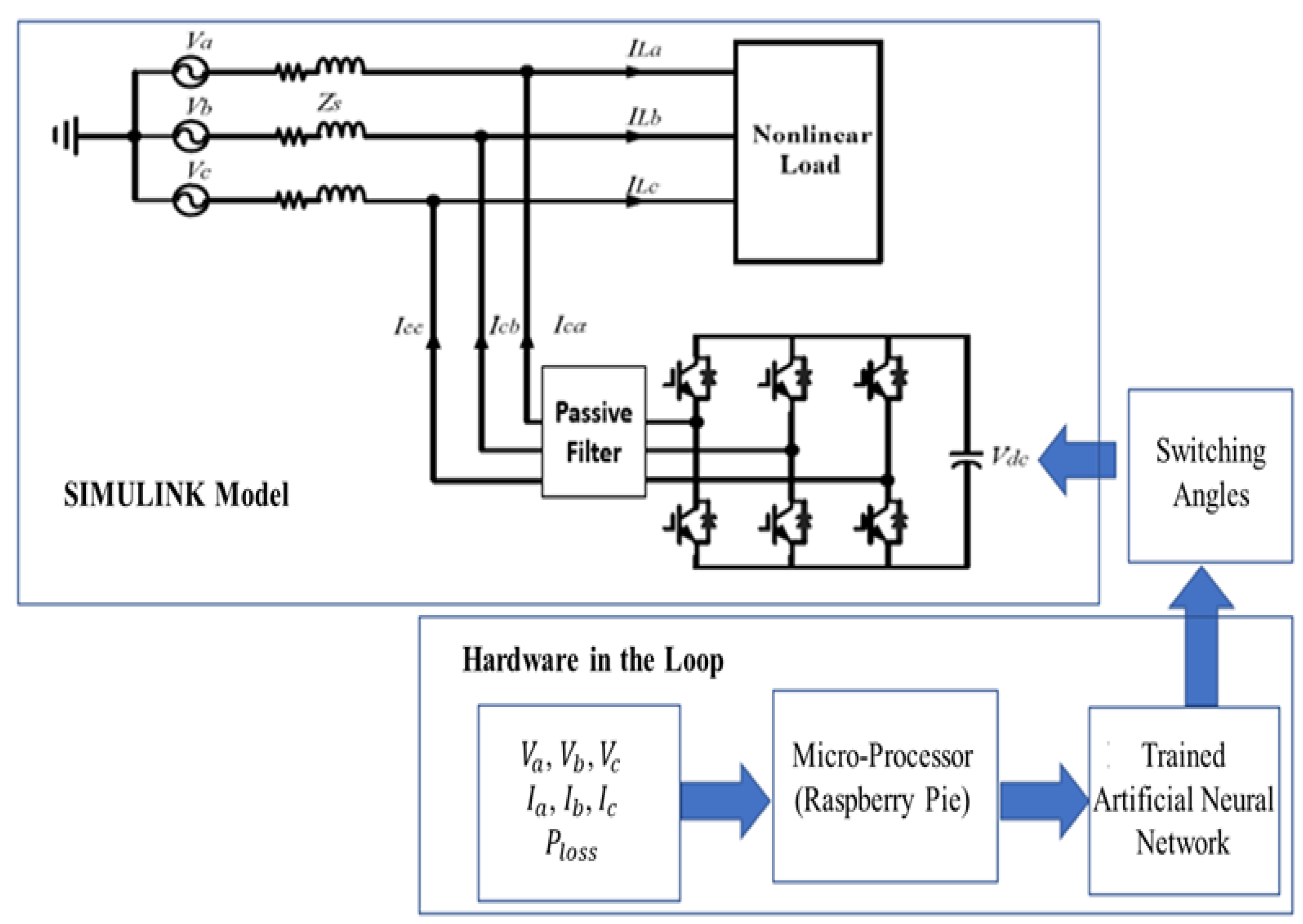
The detailed literature review motivates us to propose this work aims to develop a visual framework based on the Node RED dashboard used to monitor the process’s real-time key performance indicators (KPIs). Therefore, a three-phase HSAPF in MATLAB SIMULINK has been used to implement the HIL topology with raspberry PI 3B+ to detect the harmonics in the system and cancel the influencing neutral line current based on the generation of the required waves. Distinct topologies are used as the base of the control algorithm, namely, Pq0 based on the Clarke transformation for the synchronous reference frame theory with hysteresis control and I_d-I_q based on the Clarke and Park transformations. The comparison of their performance is made on SIMULINK. Figure 1 shows the block level system architecture of the proposed technique for the HIL-based filter.

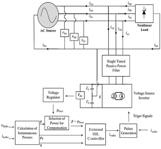
Figure 1. Block Diagram of the System Architecture.

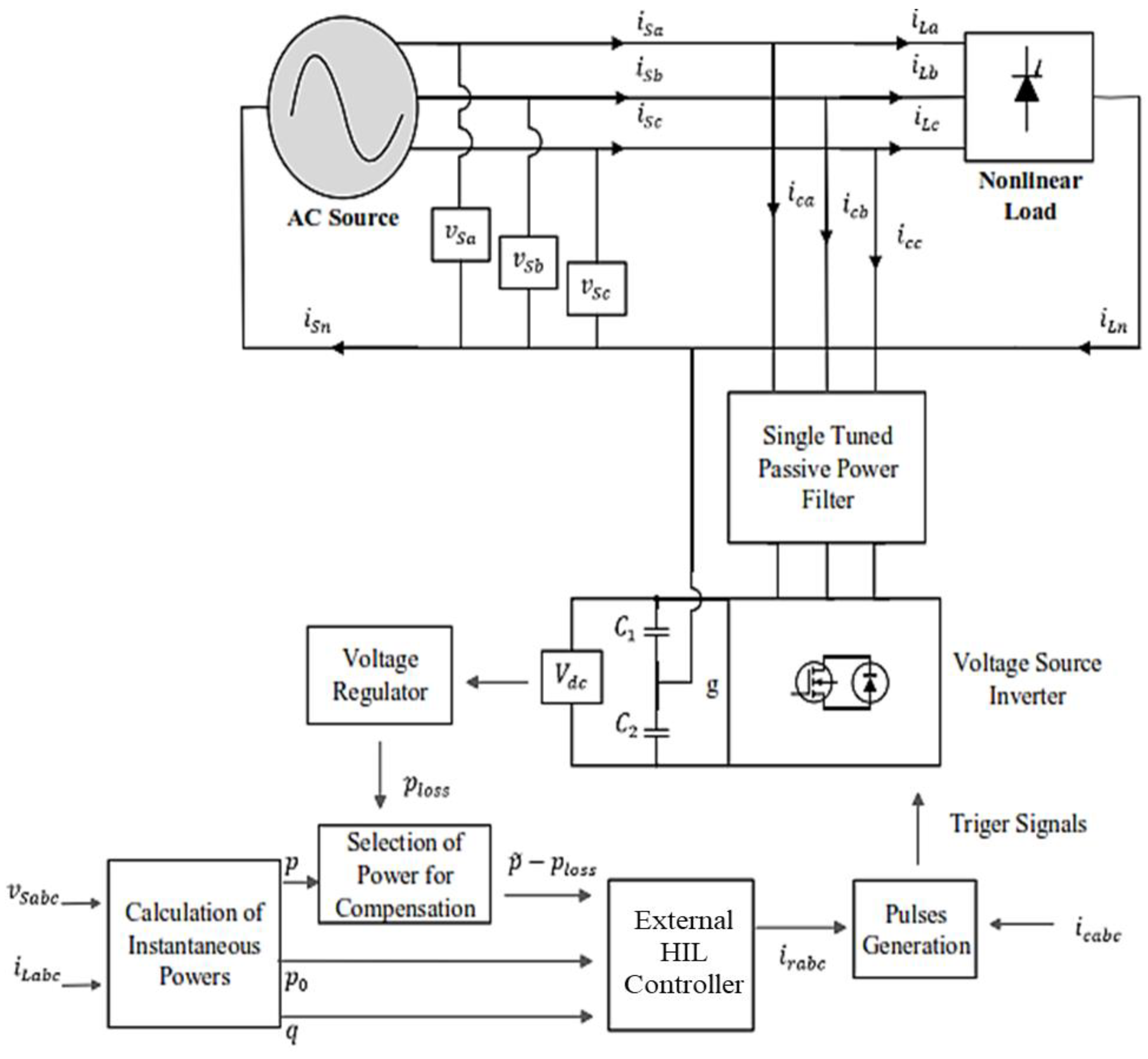
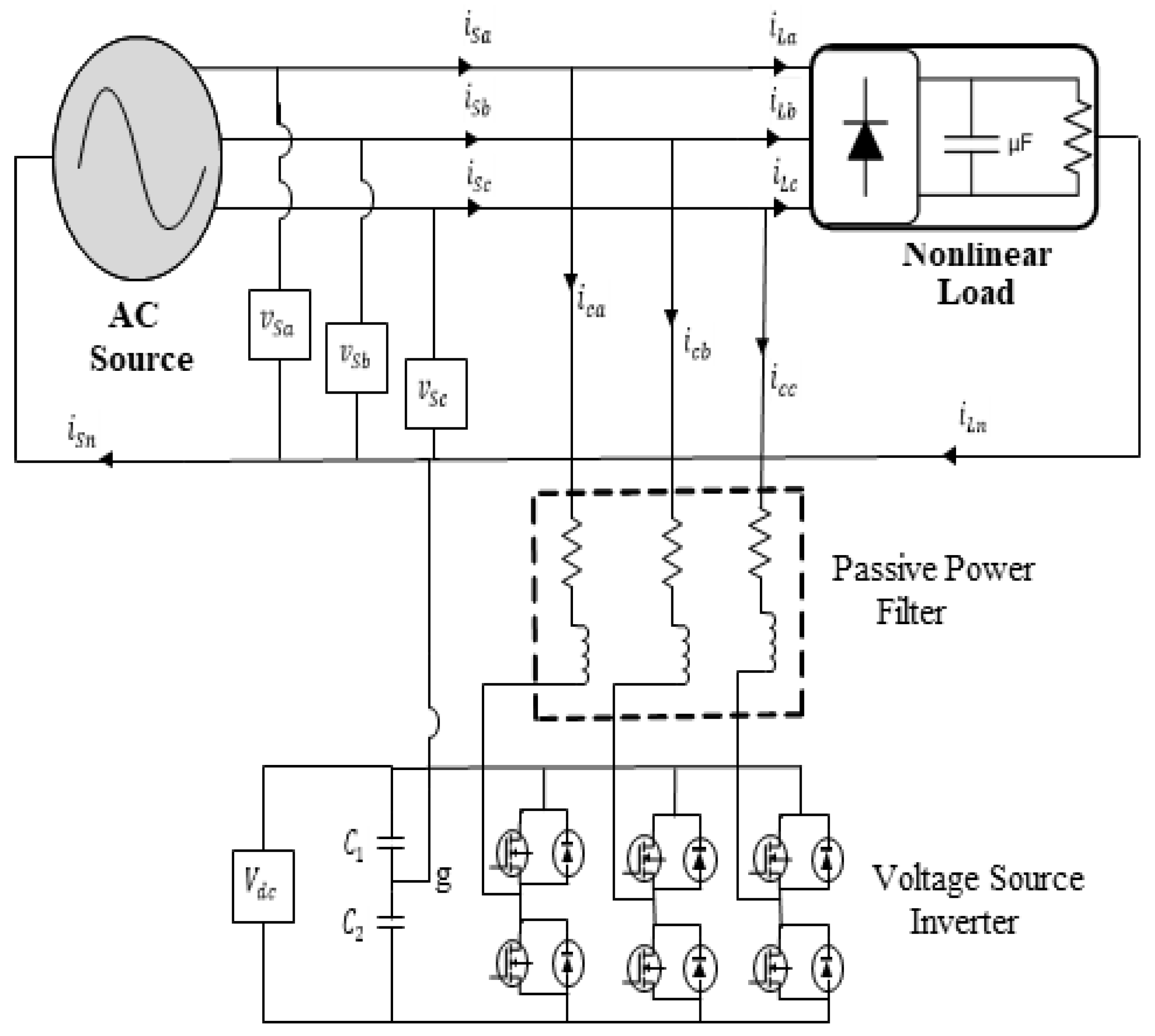
The designed model is simulated in SIMULINK, and the HSAPF control algorithm for reference current generation is implemented in a PI microprocessor. Harmonic distortion in any particular power distribution system follows a symmetric pattern regarding the power loss due to current in the neutral line of the three-phase four-electrical wire system. Hence, the proposed methodology employee an ANN in MATLAB SIMULINK for predictive analysis. The ANN is initially fed with the voltage and current signals from the bus bar infected with harmonics. Further, the network is trained to predict the reference current signal that was originated as the output of Pq0 theory. Moreover, these signals are used to generate firing angles for the switching IGBTs for inverse harmonics. HIL simulation is used to perform real-time testing of advanced control algorithms. The controller processes the analog signals to generate gate control signals and is sent back to the simulator for appropriate switching actions. The HIL is an effective platform under academic conditions that offers minimum risk, cost, and time effectiveness. The advantage HIL controller is that it provides a simulated clone of the entire physical system, including the power supply and the control circuit. The block diagram of HSAHPF has been presented in Figure 2. It shows a three-phase voltage supply that offers I_la, I_lb, and I_lc as the load currents on all three phases. Since a non-linear load is consuming the mentioned current to introduce harmonics in the distribution system, the filter uses IBGTs as switching devices to eliminate harmonics. However, to reduce the rated power of the conventional (3-pin) 6-IGBT used in APF, a single-tuned passive harmonic power filter tuned for the 5th harmonic is implemented in SIMULINK. The main purpose of the HIL test is to generate a real-time code of the reference current according to the above control algorithm. The amplitude of the current signal is equal but with an opposite phase-shifted of 180-degree. This signal is used to eliminate the influence of the distorted harmonic waveform. Based on THD and efficiency, the two SIMULINK and HIL controller technologies are compared and analyzed in detail.

Figure 2. Block Diagram of HSAHPF Configured With HIL.

Distinctive topologies persist in the literature that has been employed to mitigate harmonics, compensate for the reactive power, and improve the quality of overall power consumed. However, comparative analysis of the existing literature shows that most of the significance has been laid on developing real-time simulations for a 3-phase balanced load for integrating and testing HSAHPF. Hence the methodology of this research integrates a physically embedded processor that executes the control algorithm in a real-time environment that best suits the implementation and testing for a three-phase HSAHPF. The objective of this work is listed in the following bullets.

➢

Design of a SIMULINK model for HSAHPF based on ANN.

➢

Python scripting for hybrid active power filter.

➢

Implementation of Hardware in the loop (HIL) based environment for communication between SIMULINK and the microprocessor.

The following sections are organized as follows: Section 2 presents the power circuit topology of HSAHPF and the fundamentals of HIL implementation, conventional control techniques for hybrid filters, design parameters for power circuits, and proposed control algorithms along with their implemented model in SIMULINK and HIL controller. In Section 3, real-time simulations and results are presented that contribute to the discussion of theoretical and Experimental results verified through HIL simulations. In Section 4, a comparative analysis of both proposed and conventional techniques is discussed based on THD and HIL-implemented control algorithm’s effectiveness. Finally, Section 5 encapsulates the findings and substantial contributions of this research work.

2. Materials and Methods

This work proposes a hybrid shunt active harmonic power filter (HSAHPF) design to minimize current harmonics, improving power quality. A digital HIL controller is implemented to improve power quality. Moreover, different controlled technologies have been implemented together with Raspberry PI 3B+ to maintain cost-effectiveness and performance efficiency. The microprocessor acts as a central server that receives the polluted signal with the effects of harmonics. A compensating reference current is injected into the system to eliminate the negative effect concerning the received signals. The following subsections provide implementation details. A single-tuned PF is used for low-order load current harmonic compensation (i.e., 3rd and 5th orders) to further compensate for reactive power components caused by highly non-linear loads. The APF is mainly composed of VSI and a DC link capacitor bank. The VSI is the main part of HSAHPF that can generate reference current in cooperation with voltage regulators to compensate harmonics. Therefore, the configuration of HSAHPF effectively reduces the switching loss while maintaining the rated voltage of the APF. Moreover, it also avoids parallel resonance and series resonance. Additionally, in APF method, the DC link capacitor voltage should be kept higher than the peak-power supply voltage value to control active and reactive power fluctuations by injecting harmonic currents. So, in the HSAHPF topology, the PPF capacitor controls the basic power-side voltage across its terminals, and the APF will maintain the basic voltage on the DC link. In the proposed work, the control technique has been used in SIMULINK to implement HSAHPF. Moreover, the power circuit uses SIMULINK’s internal modeling, and the control algorithm used in a microprocessor.

2.1. Load Management in a 3-∅, Four-Wire System

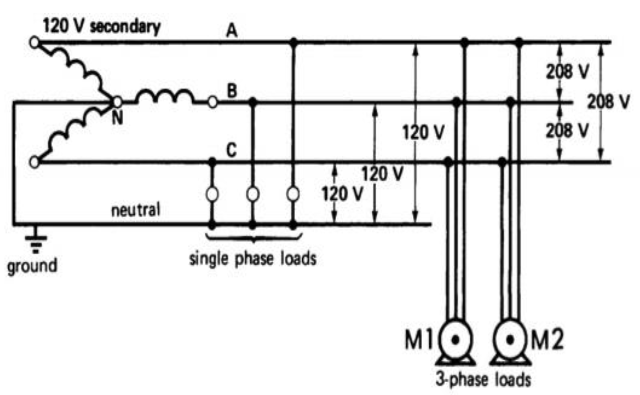
A 3-phase 4-wire power distribution systems is widely cast-off to provide power to single-phase or 3-phase loads in production plants, residential and commercial buildings. A single-phase power is provided to small-scale loads over one of the phase lines and the neutral line in these systems. This load must be evenly distributed to maintain the balance on the overall distribution system. In the case of unbalanced distribution, a net current flow through the neutral conductor. Figure 3 shows the configuration of a 3-phase load on such a system. According to the Figure, induction motor M1 and M2 are configured to distribute the electrical load evenly over the three phases. But due to the inductive motor’s non-linear characteristics, the drawn current is not equal to the three phases. Furthermore, non-linear loads (such as power electronics-based equipment) have non-sinusoidal phase currents.

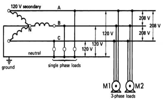
Figure 3. Three Phase Load Configuration.

However, in a well-adjusted system with harmonic distortion current waveforms, only third harmonic (the harmonic order is 3) will affect the neutral current [24]. While the harmonic distortion and load current imbalance exist simultaneously, the neutral current may contain all harmonics. Figure 4 shows a three-phase H-bridge shunt APF topology. It consists of three single-phase full-bridge (H-bridge) voltage source inverters with a common self-supporting DC bus [25]. Here, all 12 switching devices are used to realize the 3P4W shunt APF system. These H-bridge inverters are connected to the 3-phase 4-wire system by using three single-phase isolation transformers.

Figure 4. Three Phase H-Bridge Shunt APF Topology.

2.1.1. Conventional Control Methods of HSAHPF

The performance of HSAHPF is like an open circuit, used for harmonics introduced by switchgear. To introduce the simple design of HSAHPF, it is assumed that the compensator can draw any set of arbitrarily selected reference currents like a control current source. Figure 3 shows the basic principle of harmonic current compensation using filters connected in parallel.

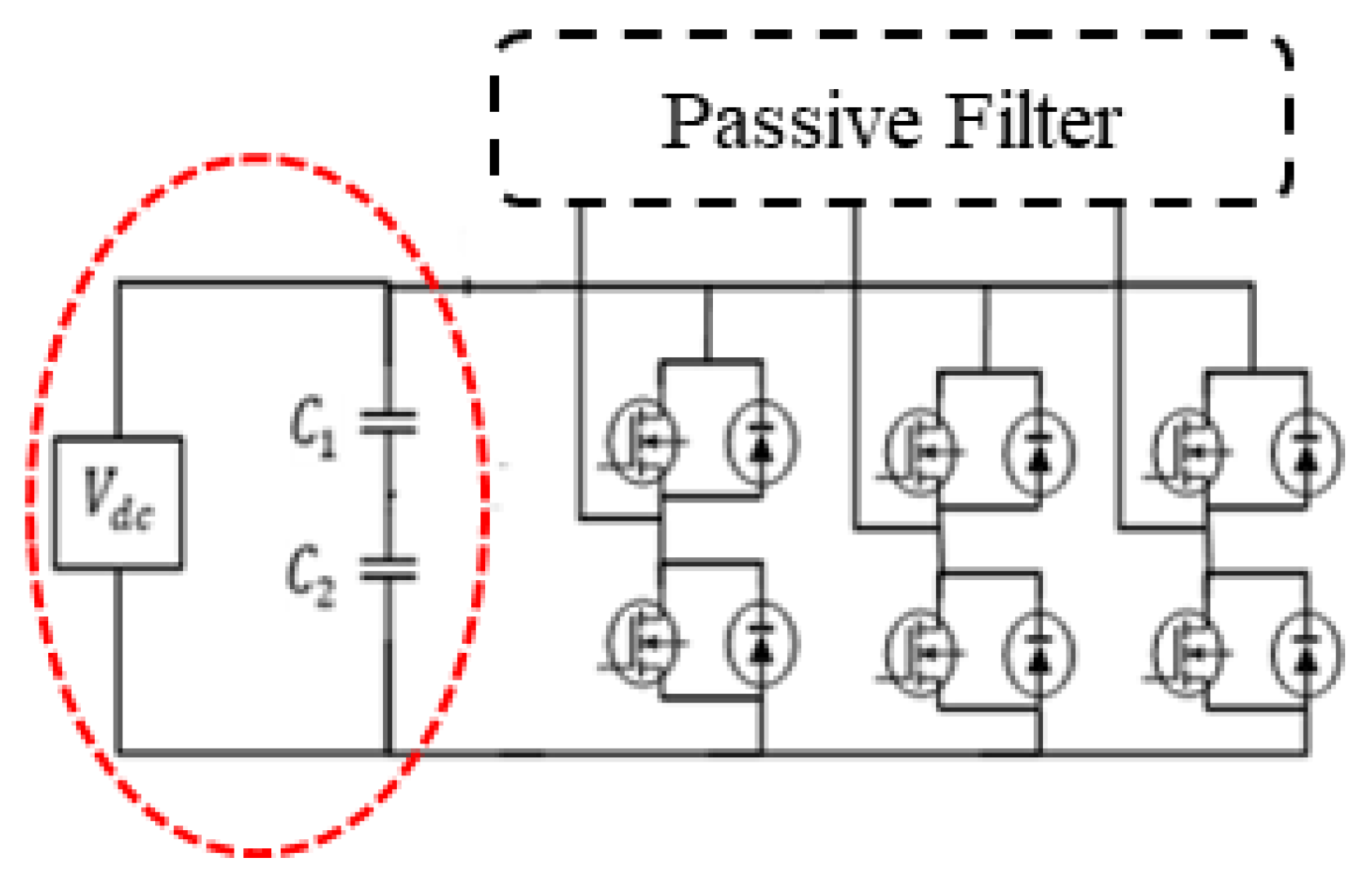
According to reactive power consumption and the prominent harmonics in the observed system, the PPF is adjusted for a specific harmonic frequency. The source current includes load current and compensation current to avoid harmonic propagation caused by PPF resonance. HSAHPF can also be used to provide continuous harmonic damping on the entire power line. The energy storage element as a VSI capacitor (Figure 5) must be large enough so that the system will not withstand large voltage changes. If the amplitude of the DC voltage is lower than the AC voltage, the converter will consequently lose control.

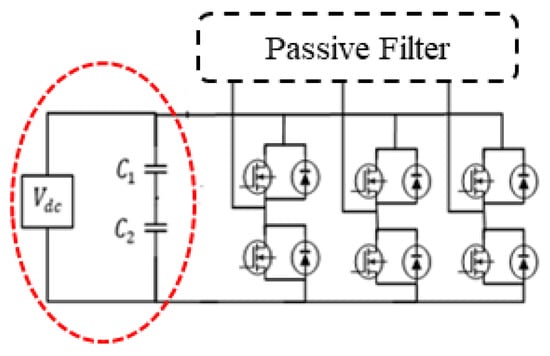
Figure 5. DC-link capacitors for IGBTs.

2.1.2. Instantaneous Active and Reactive Power Theory (Pq0)

The instantaneous power set defined in the time domain is the basis of the Pq0 theory. It is equally effective in both transient and steady-state because it can be directly applied to 3-phase and 3-wire or 4-wire systems without modification or restriction. The above theory is systematic and universal regarding the power supply filter controller design based on power electronic equipment. The two main transformations involved in this theory are as follows.

➢

Transformation of power system current and voltage from abc domain to αβ0 domain.

➢

Transformation of αβ0 domain voltage and current into active and reactive powers.

(A) Clarke Transformation

Clarke transformation involves the conversion of three-phase instantaneous current and voltage from conventional 3 phase to αβ0 coordinates. For the observed constant power case, the Clark transformation of current and voltage has been used in [25]. By implementing the invariant power form of the Clarke transform, the transformation can retain the active and reactive power of system power in a conventional reference frame. For balanced systems, zero component remains equal to zero. This conversion is based on the mathematical model provided as in (1) and (2).

$$\left[\begin{array}{c}{i}_{\alpha }\\ i_{\beta }\\ i_o\end{array}\right]=\frac{\sqrt{2}}{\sqrt{3}}\left[\begin{array}{ccc}1& -1/2& -1/2\\ 0& \sqrt{3}/2& -\sqrt{3}/2\\ 1/\sqrt{2}& 1/\sqrt{2}& 1/\sqrt{2}\end{array}\right]\left[\begin{array}{c}\begin{array}{c}{i}_a\\ i_b\\ i_c\end{array}\end{array}\right]$$

(1)

$$\left[\begin{array}{c}{v}_{\alpha }\\ v_{\beta }\\ v_o\end{array}\right]=\frac{\sqrt{2}}{\sqrt{3}}\left[\begin{array}{ccc}1& -1/2& -1/2\\ 0& \sqrt{3}/2& -\sqrt{3}/2\\ 1/\sqrt{2}& 1/\sqrt{2}& 1/\sqrt{2}\end{array}\right]\left[\begin{array}{c}\begin{array}{c}{v}_a\\ v_b\\ v_c\end{array}\end{array}\right]$$

(2)

(B) Inverse Clarke Transformation

For the conversion of αβ0 domain voltage and current into active and reactive powers, inverse Clarke transformation is employed. The mathematical model for inverse Clarke transformation is based on (3) and (4).

$$\left[\begin{array}{c}{i}_a\\ i_b\\ i_c\end{array}\right]=\frac{\sqrt{2}}{\sqrt{3}}\left[\begin{array}{c}\begin{array}{ccc}1& 0& 1/\sqrt{2}\\ -1/2& \sqrt{3}/2& 1/\sqrt{2}\\ -1/2& -\sqrt{3}/2& 1/\sqrt{2}\end{array}\end{array}\right]\left[\begin{array}{c}\begin{array}{c}{i}_{\alpha }\\ i_{\beta }\\ i_o\end{array}\end{array}\right]$$

(3)

$$\left[\begin{array}{c}{v}_a\\ v_b\\ v_c\end{array}\right]=\frac{\sqrt{2}}{\sqrt{3}}\left[\begin{array}{c}\begin{array}{ccc}1& 0& 1/\sqrt{2}\\ -1/2& \sqrt{3}/2& 1/\sqrt{2}\\ -1/2& -\sqrt{3}/2& 1/\sqrt{2}\end{array}\end{array}\right]\left[\begin{array}{c}\begin{array}{c}{v}_{\alpha }\\ v_{\beta }\\ v_o\end{array}\end{array}\right]$$

(4)

Both Clarke transformation and its inverse transform are power invariant. In a three-phase system, this feature has been preferred to monitor the instantaneous power. The transformation of instantaneous voltage and current from 3-∅abc to ∅αβ0 axes of the active power (p), imaginary power (q), and zero sequence power (p0) is defined in (5).

$$\left[\begin{array}{c}p\\ q\\ p_o \end{array}\right]=\left[\begin{array}{ccc}0& v_{\alpha }& v_{\beta }\\ 0& v_{\beta }& -v_{\alpha }\\ v_o& 0& 0\end{array}\right]\left[\begin{array}{c}{i}_o\\ i_{\beta }\\ i_{\alpha }\end{array}\right]$$

(5)

Further, the inverse of the above transformation can be modeled as in (6)

$$\left[\begin{array}{c}{\mathrm{i}}_{\mathrm{a}}\\ {\mathrm{i}}_{\mathrm{b}}\\ {\mathrm{i}}_o\end{array}\right]=\frac{1}{{\mathrm{v}}_{\mathrm{o}}\mathrm{A}}\left[\begin{array}{c}\begin{array}{ccc}{\mathrm{v}}_{\mathrm{o}}{\mathrm{v}}_{\mathsf{\alpha }}& {\mathrm{v}}_{\mathrm{o}}{\mathrm{v}}_{\mathsf{\alpha }\mathsf{\beta }}& 0\\ {\mathrm{v}}_{\mathrm{o}}{\mathrm{v}}_{\mathrm{b}}& -{\mathrm{v}}_{\mathrm{o}}{\mathrm{v}}_{\mathsf{\alpha }}& 0\\ 0& 0& \mathrm{A}\end{array}\end{array}\right]\left[\begin{array}{c}\begin{array}{c}\mathrm{p}\\ \mathrm{q}\\ {\mathrm{p}}_o\end{array}\end{array}\right]$$

(6)

where;

$$A = {v_{\alpha }}^2+{v_{\beta }}^2$$

In the time domain, the complement of Pq0 theory is inconsistent with traditional theory in the frequency domain. It can thoroughly analyze a three-phase system and calculate all power and current in real-time. It detects and eliminates all the unwanted currents simultaneously, thereby improving system efficiency [26]. A power system with current harmonics can eliminate all currents with undesired frequencies by introducing a current with the same amplitude but with a 180° phase shift in the undesired current waveform system currently is a sine wave. The system can eliminate the current harmonics by introducing a current with identical amplitude but a phase shift of 180° in the undesired current waveform.

2.1.3. Parameters and Proposed Control Techniques

The efficiency of the proposed HSAHPF using a control algorithm to mitigate current harmonics due to the presence of non-linear loads has been performed by using MATLAB/SIMULINK. Additionally, to evaluate the performance of the proposed control algorithm, 10 KVA, 220 V, HSAHPF were implemented on a 50 Hz basic frequency to improve power quality. Table 2 lists the description, parameters, and specifications of the system under study.

Table 2. Design parameters of Simulated Environment.

Simulation Parameters	Values
Phase voltage RMS value	220 V
Frequency	50 Hz
${\mathit{R}}_{\mathit{f}}$	$1 \mathrm{m}\mathsf{\Omega }$
${\mathit{L}}_{\mathit{f}}$	$3 \mathrm{m}\mathrm{H}$
${\mathit{C}}_{\mathbf{1}}={\mathit{C}}_{\mathbf{2}}$	$470 \mathsf{\mu }\mathrm{F}$
${\mathit{V}}_{\mathit{r}\mathit{e}\mathit{f}}$	622 V DC
${\mathit{k}}_{\mathit{p}}$	25
${\mathit{k}}_{\mathit{i}}$	17
Power rating	10 kVA
3 Single-phase rectifier non-linear load (R, L, and C)	$43.2 \mathsf{\Omega }$$, 34.5 \mathrm{mH}$$, 392 \mathsf{\mu }\mathrm{F}$, (720 VAR)

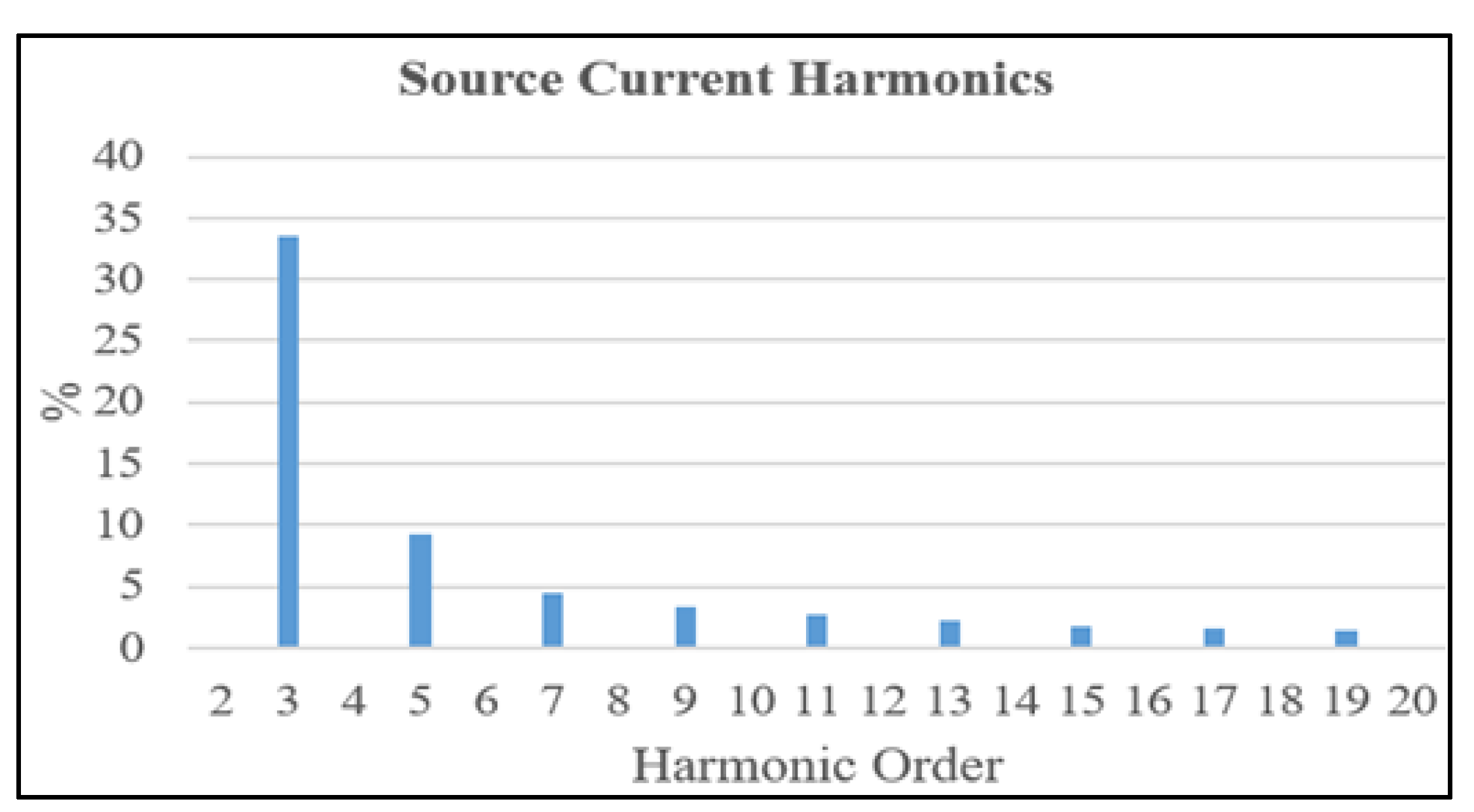
Figure 6 lists the first 20 harmonics of source current signals. For HSAHPF, to reduce the cost and rated power of APF, the PPF eliminates the 5th harmonic. Except for the third harmonic, the active power filter eliminates all other ordered harmonics. In this case, APF acts as a harmonic isolator in the system between source and load by forcing load current to flow into PPF. Figure 6 presents the source current harmonics when no filter is employed. It has been observed from the FFT analysis of waveform that the total THD of the system source current is 33.84%, which is not within the range determined by the international standard IEEE 519–1992 for the realization of current harmonics. The THD of the source voltage is 0.017%, which is already within the acceptable harmonic range defined by IEEE standards.

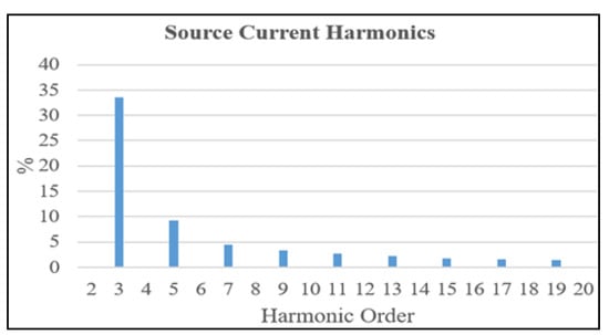
Figure 6. Source Current Harmonics When No Filter Is Employed.

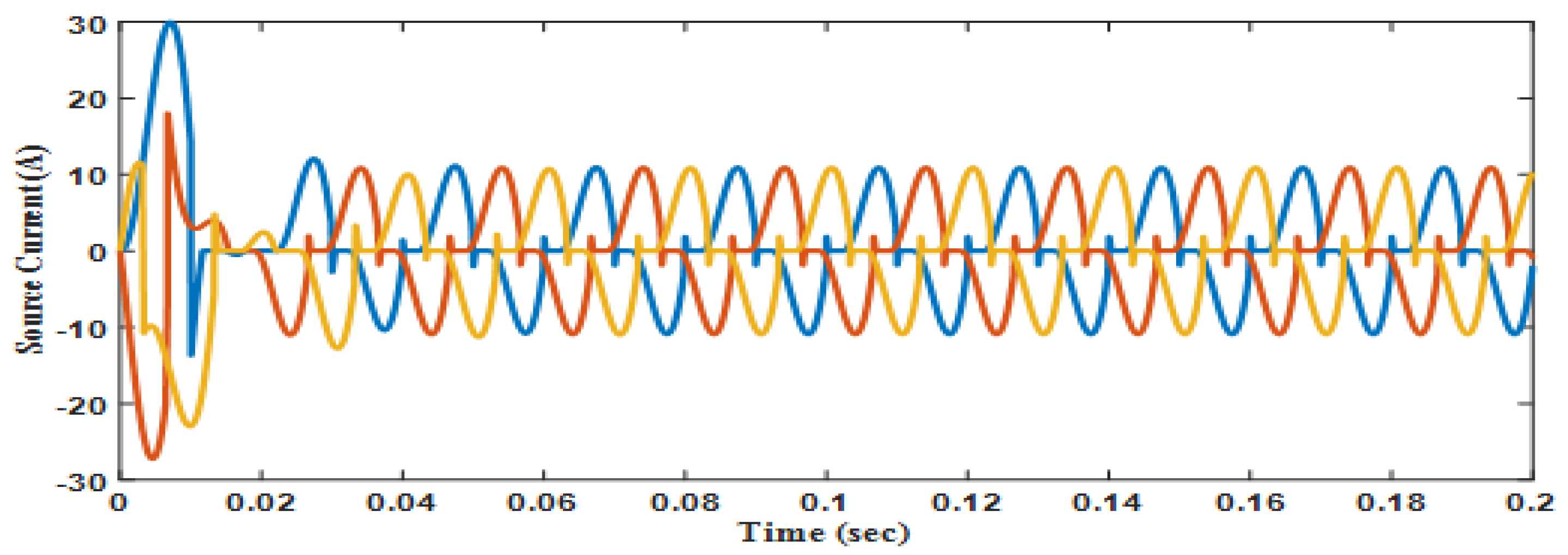
Therefore, there is no need to further enhance the source voltage waveform, but there is an urgent need to improve the source current to keep the THD within the standard range. Figure 7 shows the source current waveforms. In a three-phase, four-wire system. It is the current drawn by the source when no filter is integrated. Due to the non-linear load, the source current is not a sine wave and contains spikes due to the charging and discharging of the capacitor connected to the VSI.

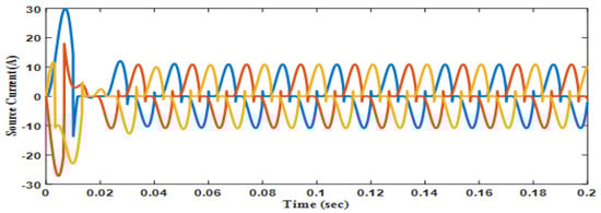
Figure 7. Source Current Waveforms.

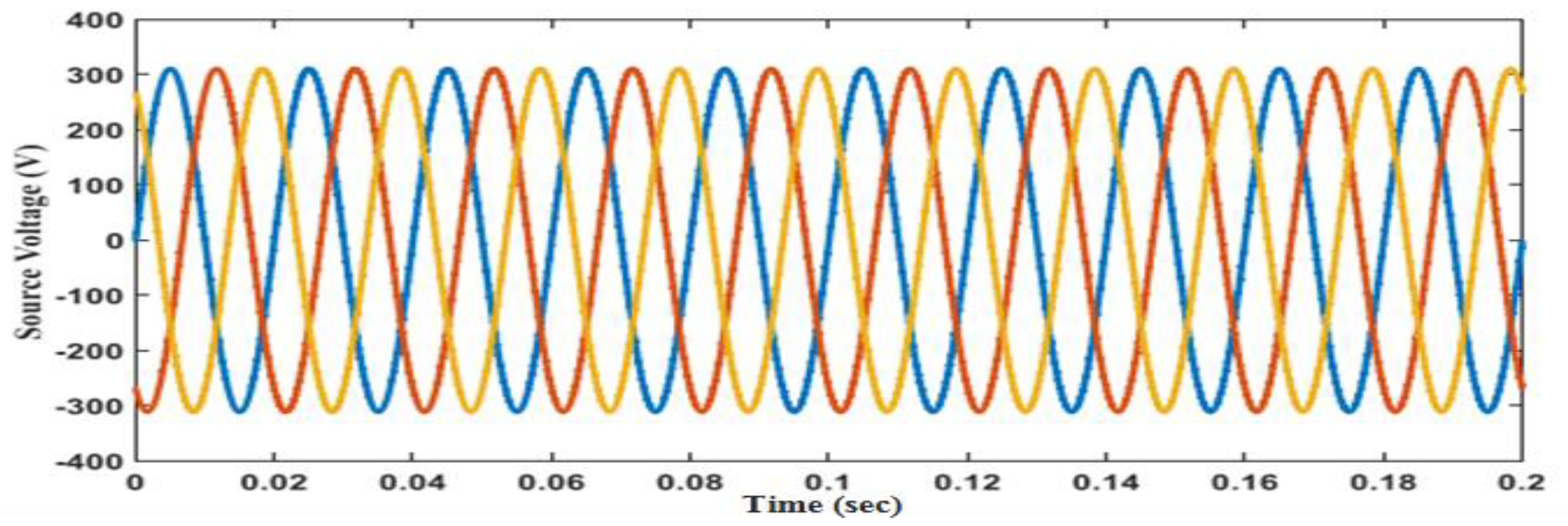
Figure 8 depicts the power supply voltage when a three-phase system has been used without HSAHPF. The waveform of the source voltage is sinusoidal because the three-phase load is evenly distributed. It can be seen that the source voltage does not contain any harmonics, so they do not play any role in the pollution of the power system. Source current harmonics is the main source of the increase in % THD. In the proposed work, the major target is to interface MATLAB SIMULINK with a microprocessor (Raspberry PI). Following this approach, the algorithm based on neural networks scripted in the microprocessor generates reference current signals based on real-time inputs. The generated reference current injected back to the simulated environment generates inverse harmonics through hysteresis control. Initially, the performance of the employed control algorithms has been monitored based on simulation to match the industrial standards. However, for the physical implementation of the proposed system, it is significant to employ a processor as a central control unit. HIL configuration proves to be very helpful for this scenario as it allows the micro-processor to be integrated with the simulated environment. Moreover, it also encapsulates certain other problems in hardware development because errors and uncertainties may cause interference and uncertainties in measurement and instrument sensors.

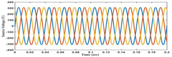
Figure 8. Source Voltage waveforms.

Along with that, Raspberry PI acts as a transceiving device since it communicates with SIMULINK and connects to the visualization server (Node-RED) for data visualization. This server acts as a historian database used to visualize the incoming and outgoing data and manage a single cycle in parallel.

2.1.4. SIMULINK Based Implementation of Pq0 Control Technique

Initially, Pq0 based HSAHPF was implemented in SIMULINK using a three-phase, four-wire that contains the following four functional blocks.

➢

DC Voltage Regulator.

➢

Calculation of instantaneous powers.

➢

Selection of power for compensation.

➢

Calculation of reference currents.

The DC voltage regulator regulates the excessive part of real power (Ploss) to maintain the voltage of the capacitor (V_dc) close to the reference DC link voltage (V_ref).

Suppose power loss (ploss) is not continuously drawn from the power circuit of the PWM-controlled converter to provide the loss caused by the switching operation. In that case, the DC capacitors (C₁ and C₂) will only continue to discharge rather than continue the cycle of charging and discharging [27].

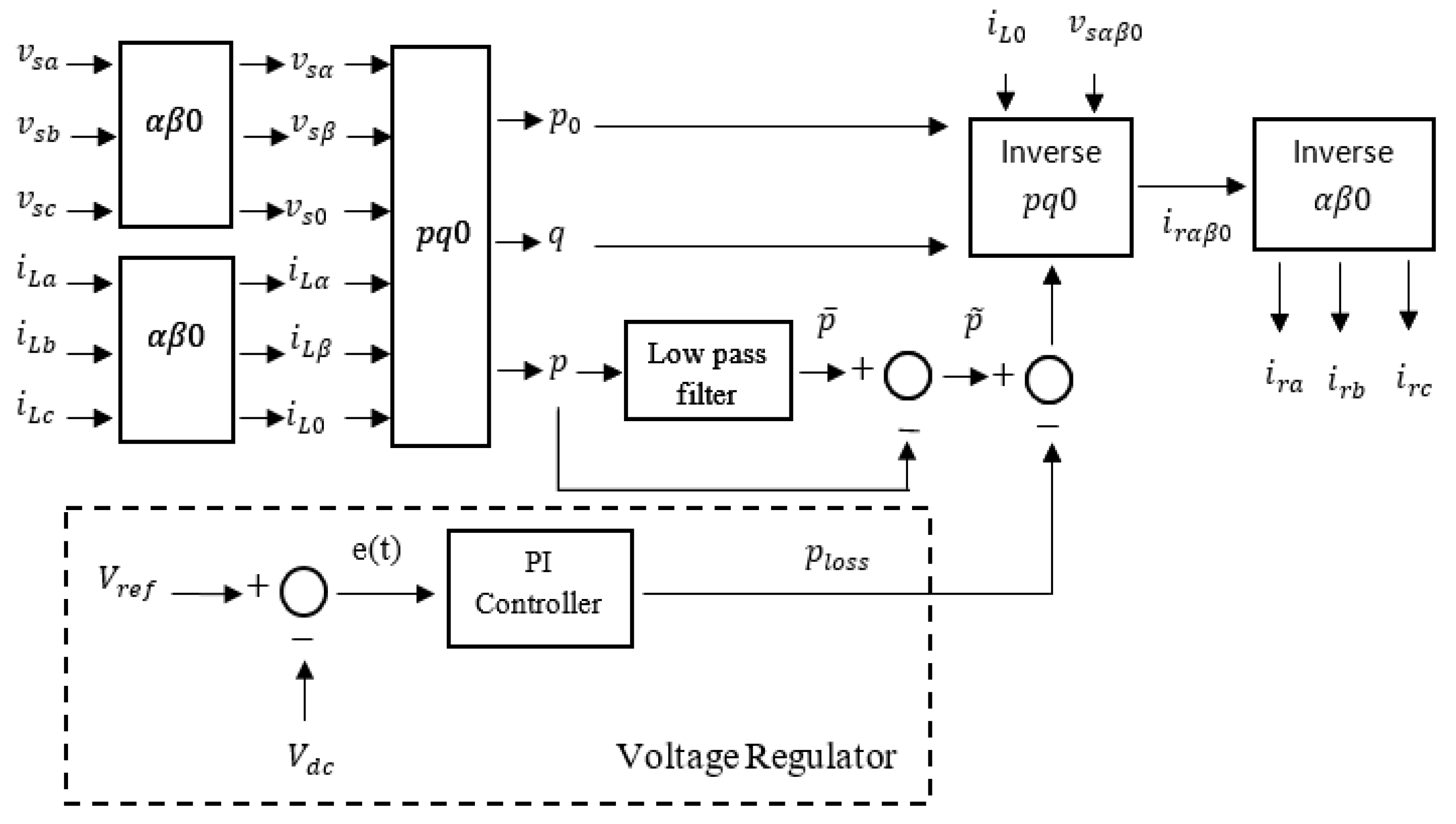
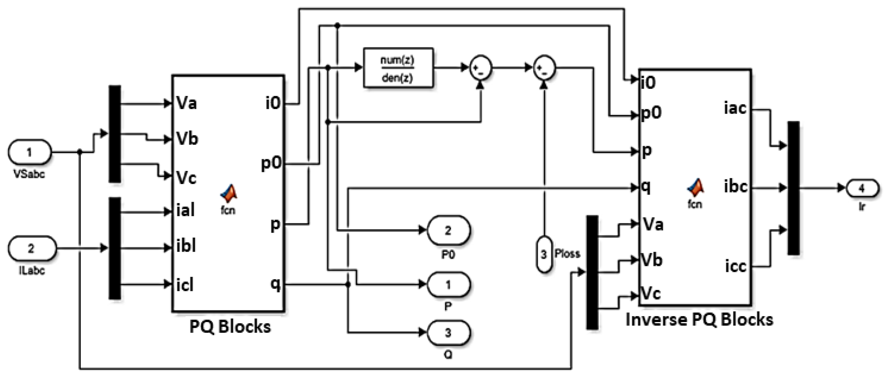
The second block includes the selection of non-linear load power, which is compensated by the influence of the low-pass filter and the DC voltage regulator. This control block uses V_sabc (V_sa, V_sb, V_sc), I_Labc (I_La, I_Lb, I_Lc) as input. As shown in Figure 9, after transforming V_sabc and I_Labc, the zero-sequence active power (p0), reactive power (q), and active power (p) is calculated, and p_loss is subtracted from the low-power active power output through filtering. The filter is fed into the inverse Pq0 block and the compensated reactive power (q) to provide the final output. It is found that the fourth-order low-pass filter is suitable for separating the active power into the average value ($\stackrel{-}{\mathrm{p}}$) and the oscillation part ($\tilde{\mathrm{p}}$). The average part of instantaneous active power in output will be separated by a low-pass filter and given p, which can be seen from the HSAHPF control activity displayed in Figure 9. The third block uses the instantaneous compensation power i0 and the phase voltage to calculate the reference current. The power circuit of the active filter part is composed of a centrally divided VSI, which is composed of 6 MOSFETs with freewheeling diodes. The performance of the VSI combined with the hysteresis controller and PWM is like that of a controlled current source (CCS). The user-defined function blocks are scripted in MATLAB SIMULINK based on a mathematical model of pq0 theory. Moreover, Figure 10 shows the designed model for the control algorithm. The output of this control block is the reference current signal. Further, the hysteresis control algorithm is used to generate a gating signal for VSI switching. As a result, the THD for the source current has been reduced significantly that dwell within the acceptable range of IEEE standards. In further, Figure 11 shows the obtained output from MATLAB SIMULINK.

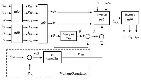
Figure 9. Pq0 theory-based comprehensive control activity.

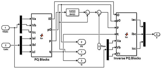
Figure 10. SIMULINK Design for PQ-theory Control Algorithm.

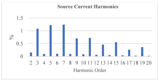
Figure 11. Source Current Harmonics with PQ-Theory Control Algorithm.

2.2. Predictive Analysis

Generally, the pq0 theory is used to calculate the reference current, and the PI controller is used for the voltage regulator. However, the methodology in this paper proposes a neural network-based predictive control scheme. This scheme is based on ANN for the design of the control block. The performance pf Pq0 theory is adequate until the supply voltage is in the ideal state [28], but the linear mathematical model of the system is necessary for the design of PI controllers. It is difficult to obtain and may not be suitable for providing the required performance under load shifting [29]. The PI controller cannot respond quickly because of the non-linear characteristics. Therefore, ANN-based algorithms provide fast, accurate, and dynamic responses for non-linear systems containing uncertain information. Therefore, this technique has been considered a more suitable alternative to the conventional method. The control algorithm that is based on predictive analysis is subdivided into two major steps. These steps are mentioned below: (a) Implement a simulated environment based on ANN in MATLAB SIMULINK. (b) Integration of HIL architecture that comprises python script on raspberry PI for the environment.

2.2.1. Simulated Environment Based on ANN in MATLAB SIMULINK

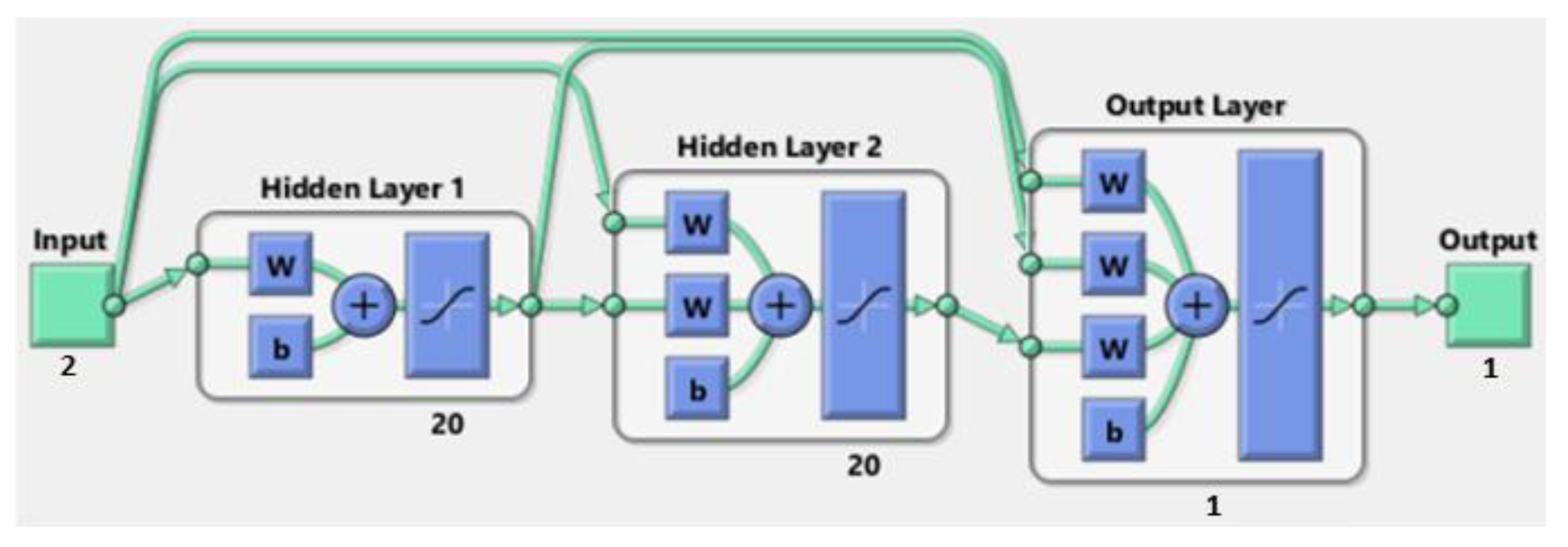
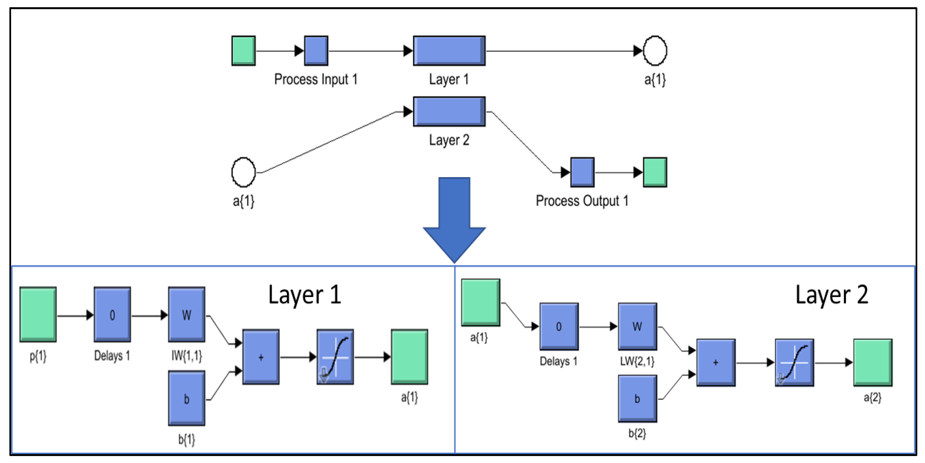
As shown in Figure 12, two hidden layer architectures each have 20 neurons for harmonic detection in SHAPF used to train cascaded ANN architecture. While training ANN, gradient descent with momentum has been used as a learning function. Moreover, the Levenberg Marquardt training function has been used to optimize weights and bias values in the used architecture. The activation function used in ANN architecture training is tan sigmoid.

Figure 12. ANN Model for Reference Current in SIMULINK.

Among the seven inputs used, three 3-ϕ source voltages (V_sa, V_sb, V_sc), three 3-ϕ load currents (i_La, i_Lb, i_Lc), and the seventh input is p_loss variable obtained from voltage regulation [29]. The harmonic reference currents (i_ra, i_rb, i_rc) are the three outputs of ANN. Similarly, ANN of the voltage regulator using two inputs (V_ref and V_dc) and one output (p_loss), using two hidden layers to carry 20 neurons, respectively, as shown in Figure 13. The trained block of ANN is further applied to the simulated environment to obtain results on a simulation basis. As highlighted in Figure 14, the seven signals used to train the network are fed as input. Following the trained weights, the ANN generates a 3-phase current as a reference signal (I_r).

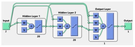
Figure 13. ANN Model for Regulated Voltage.

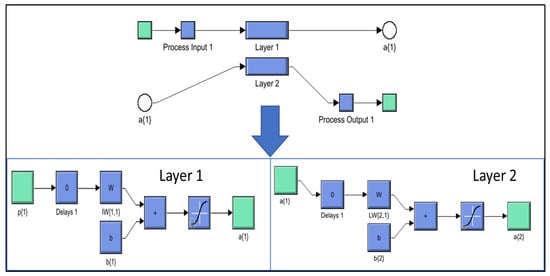
Figure 14. ANN Block and Hysteresis block in Simulink.

This reference current generated by the ANN block is received as an input by the hysteresis current control block highlighted in Figure 15. The block that receives the second input is filter current (ICabc). The hysteresis block calculates the variance between the incoming two signals. Hysteresis current controller block is configured to produce a high binary output when the calculated variance exceeds the boundary of positive or negative hysteresis band, as shown in Figure 15. Therefore, the controller will react quickly to any deviation from the control reference value; that is why these controllers have high gain characteristics. The hysteresis current controller provides binary output [30]. This binary signal provides a switching sequence for the IGBTs that are used in the VSI. The VSI can inject inverse signals concerning these switching frequencies, which eradicate the harmonics caused by non-linear load on the source current.

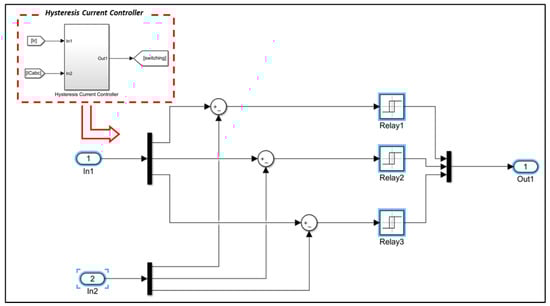
Figure 15. Hysteresis Current Controller In SIMULINK.

As shown in Figure 14, the output of the ANN control block is the reference current (Ir). So, initially, the output signal is disabled to monitor the harmonics with the control algorithm. Figure 16a shows the harmonics in the source current without Ir. In further, to monitor the effectiveness of the control algorithm on the generated harmonics on the source side, the output of the control block is enabled that reduces the harmonics significantly. Moreover, Figure 16b represents the reduced harmonics on source current after applying the ANN algorithm.

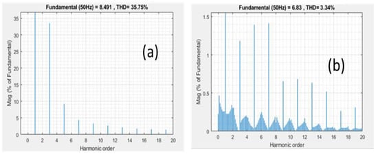
Figure 16. (a) Harmonics without control signal. (b) Harmonics with a control signal.

2.2.2. Integration of HIL Architecture on Raspberry PI

As shown in Figure 16, the ANN algorithm efficiently reduces the % THD of the source current. As the complete topology has been based upon simulations hence, to inculcate and test the working of a physical processor, HIL-based architecture is implemented. In this architecture, the ANN control algorithm is scripted in Raspberry PI 3B+ that receives input from the simulation and provides reference current for the hysteresis control block as an output signal. The system architecture for the HIL configuration has been provid4ed in Figure 17.

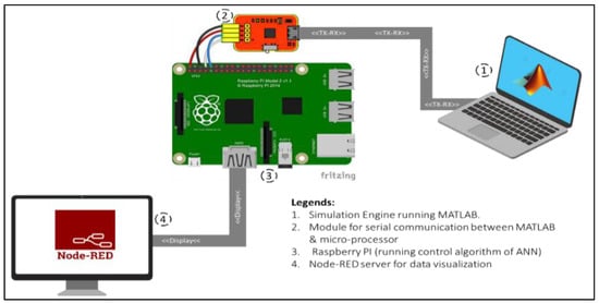
Figure 17. System Architecture for HIL with Microprocessor.

Initially, for implementing HIL-based architecture, an ANN-based control algorithm has been scripted for the microprocessor. For this algorithm, the tensor flow library of machine learning has been employed that supports backpropagation topology to train ANN to predict desired results with a defined learning rate. Generally, the training of neural networks [31] comprises the following 6 stages:

(a)

Initialization;

(b)

Forward propagation;

(c)

Cost function formulation;

(d)

Backpropagation;

(e)

Weights update;

(f)

Iteration until convergence.

Stage 4 (backpropagation) reduces the error that maintains the cost function [32]. It calculates the difference between actual and desired outputs of the network. Moreover, it also calculates the degree to which the sequential outputs are affected by the discrete weights. The backpropagation uses partial derivate to obtain the rate of change from the cost function to the neuron assigned with a specific weight. The backpropagation algorithm calculated the 3 partial deviates include a derivative of total errors for desired output, a derivative of desired output for a total input of the neuron, and a derivative of the input for a hidden neuron with the assigned weight. The Leibniz Chain Rule calculates the optimal value of a specific weight that minimizes the error function based on these derivatives.

2.3. Modeling of the Artificial Neural Network

The functionality of backpropagation has been segregated into two parts: Activation and Optimization to implement this algorithm in a tensor flow environment for the microprocessor.

2.3.1. Comparison of Activation Functions

While the training process of the ANN model for the control algorithm of hybrid harmonic power filter 8 distinct Keras activation function is compared based on Mean Square Error (MSE) and validation efficiency, the comparison has been performed on a fixed value of 300 epochs. Table 3 shows the results obtained based on this comparison.

Table 3. Comparative analysis of activation functions.

Sr No.	Activation Function	Efficiency	MSE	Epochs
1	sigmoid	0.96	0.0012601	300
2	softmax	0.54	0.0897195	300
3	Elu	0.99	0.0002285	300
4	exponential	0.94	0.0034175	300
5	softplus	0.94	0.0012314	300
6	softsign	0.98	0.0000675	300
7	tanh	0.98	0.0002923	300
8	relu	0.99	0.0000166	300

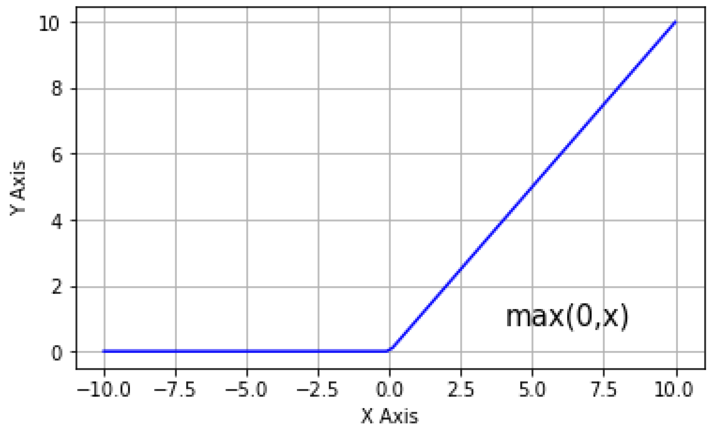
It is required to eradicate the negative input values and a linear output for the positive values to activate weights of inputs in the designed network. Hence, this functionality is best suited by Rectified Linear Unit (ReLU) activation function. Since the variance in the incoming input signals is very small, the slope of the gradient descent of the ReLU function shown in Equation (7) minimizes the probability of data loss.

$$R\left(z\right)=\max \left(0,z\right)$$

(7)

Sparsity in the ReLU function best suits the limited microprocessor hardware architecture due to less computational cost. Figure 18 provides the graphical representation of the generic ReLU activation function. The Figure shows the output is zero for negative input and linear for positive inputs.

Figure 18. Graphical Representation of Generic ReLU Activation Function.

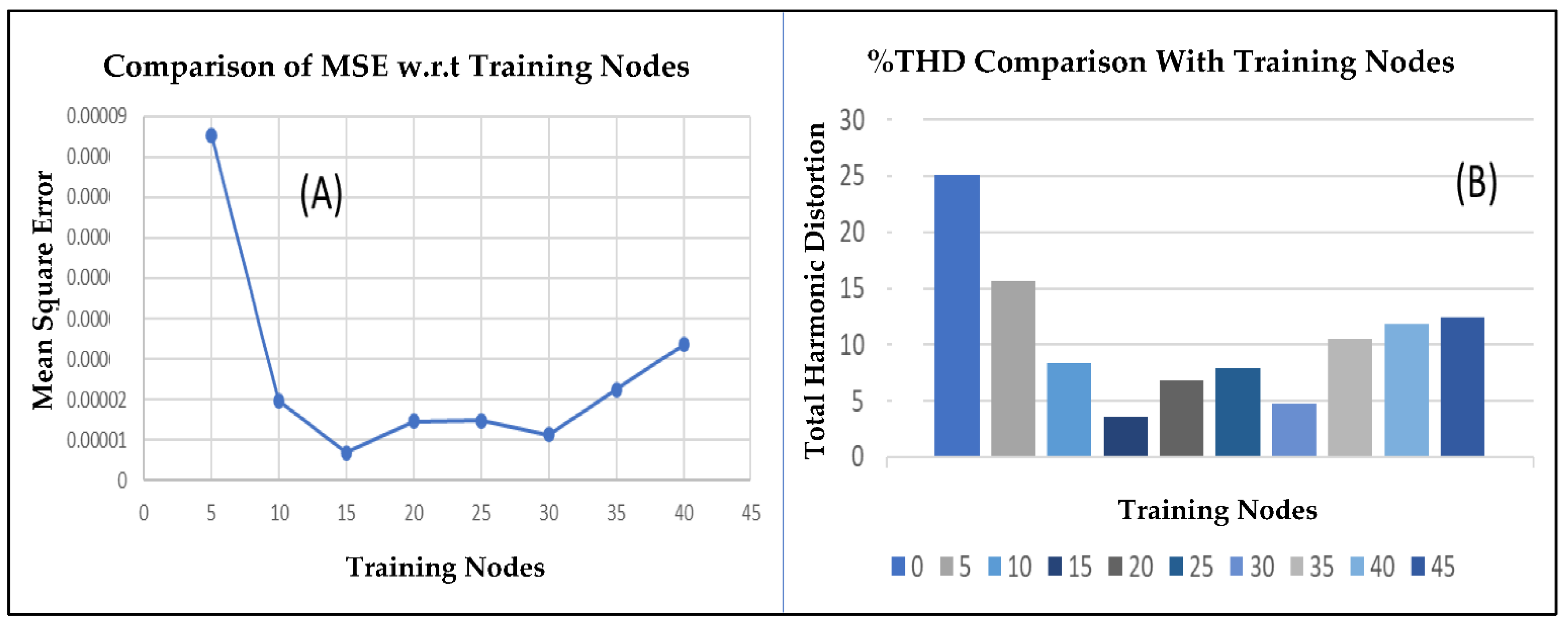
2.3.2. Selection of Nodes in Hidden Layers

An iintuitive method is used to select nodes for the 2 hidden layers of the neural network. Figure 19A shows the efficiency comparison with selecting a different number of nodes, while Figure 19B shows the comparison of %THD for the training nodes. This comparison shows that the least amount of MSE is obtained with 15 nodes per hidden layer. So, the neural network is trained with the ReLU activation function (Table 2) and 15 nodes per hidden layer.

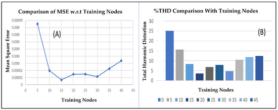
Figure 19. (A) MSE Versus Training Nodes. (B)% THD Versus training nodes.

2.3.3. Selection of Optimal Optimizer

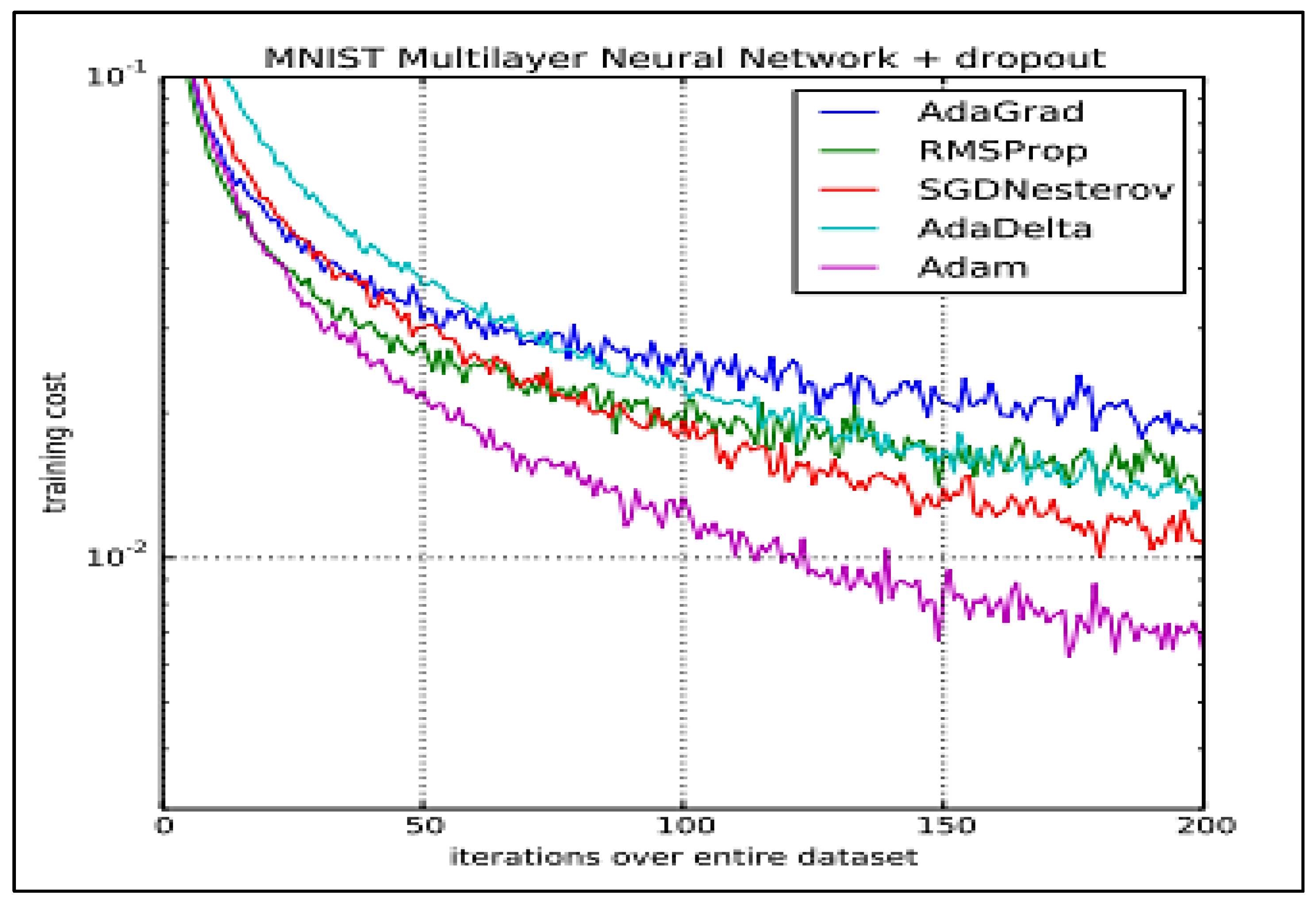
After completing a single cycle that starts from incoming input signals, their multiplication with arbitrary weights, and then passing through the activation function to produce output, the next step is optimization. Optimization aims to minimize the cost function. In other words, the optimizer reduces the Mean Square Error (MSE) by using the square of the difference between the actual and predicted outputs. The lower the difference, the more accurate the prediction would be. Conventionally, stochastic gradient descent optimization is used in machine learning applications. However, the stochastic gradient descent maintains a unique learning rate for all the weight updates and does not change during training. It leads toward declaring a local minimum instead of a global minimum of an entire data set. As a result, it introduces errors during the training process of the ANN. An Adaptive Moment Estimation (ADAM) optimizer has been used to overcome this problem. It is an optimization algorithm used as an extension of the conventional stochastic gradient descent algorithm.

Moreover, it combines the following distinct topologies of gradient descent.

➢

Adaptive Gradient Algorithm (AdaGrad)

➢

Root Mean Square Propagation (RMSProp)

Figure 20 shows a comparative analysis of various optimizers. The comparison represents the performance of each optimizer in reducing the cost function concerning each iteration in the data set.

Figure 20. Comparative Analysis of Optimizers in TensorFlow.

Root Mean Square Propagation (RMSProp) uses the average first moment (the mean) to adapt the parameter learning rates. Alternatively, ADAM uses the first and second moments of the gradient to adapt the learning rates [33]. This method can calculate an exponential moving average of the gradient and the squared gradient, allowing the algorithm to handle sparse gradients on noisy problems.

As shown in Figure 21, the MSE is reduced to 0.00033% when the designed ANN is trained up to 600 epochs. The next step in implementing HIL is to feed the input signals from the simulated environment (SIMULINK) to the trained model. After receiving the input signals, the trained model would generate reference current as output would be fed back to the simulated environment as the input signal for the hysteresis block. Two respective blocks would therefore replace the ANN control block. (1) TCP/IP Client send and (2) TCP/IP Client receives.

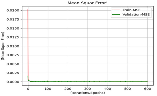
Figure 21. Mean Square Error After ANN Training.

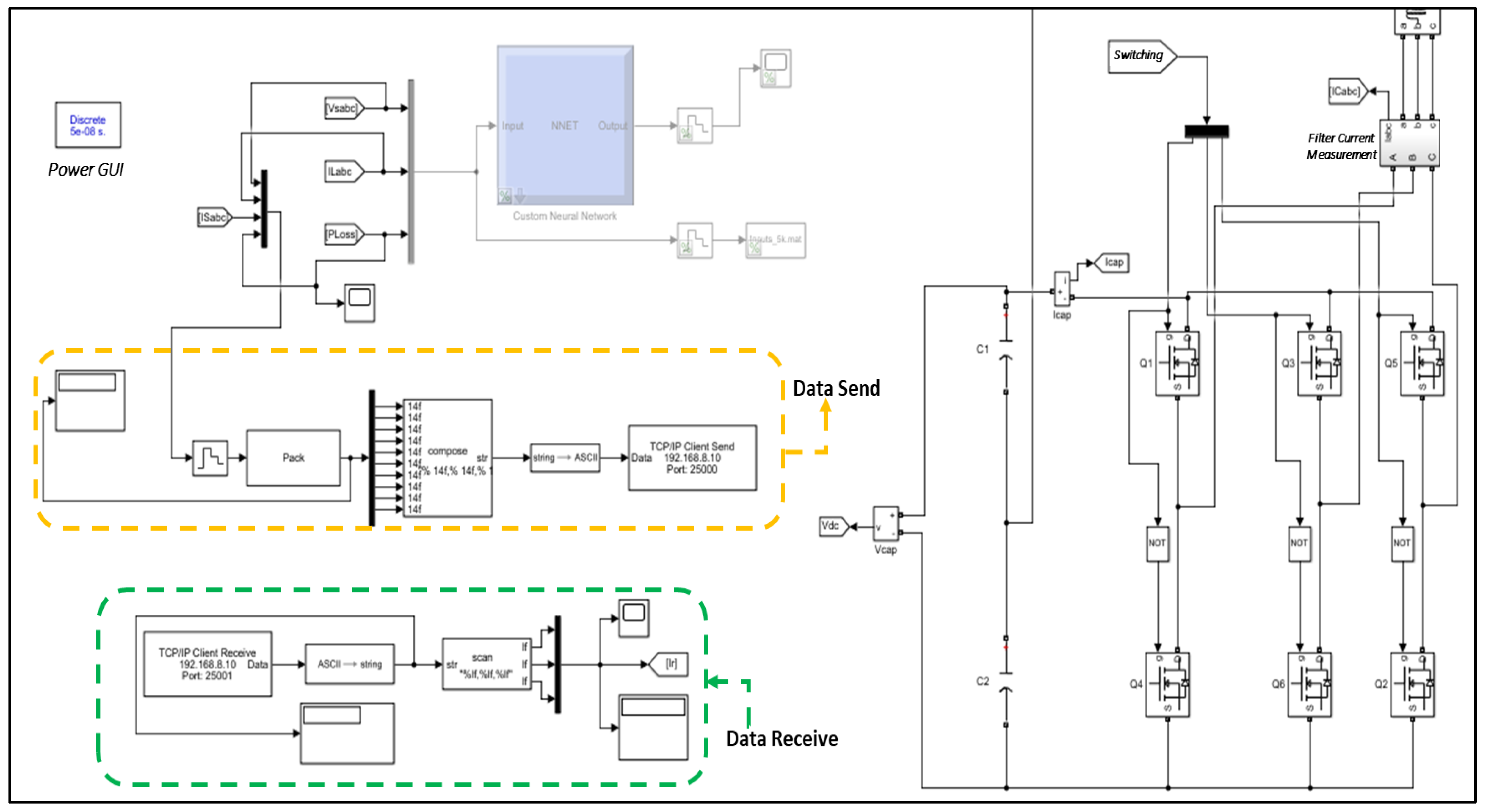
The first one would send the input signals (3-phase source voltage, 3-phase load current and the compensated signal from voltage across the DC link capacitors) to the trained model in the microprocessor. The second block would receive the 3-phase reference, which is the output from the microprocessor through the trained network. Moreover, Figure 22 illustrates the integration of these two blocks within the simulated environment. The yellow highlighted block shown in Figure 22 sends the seven input values to the microprocessor over a specified TCP/IP port.

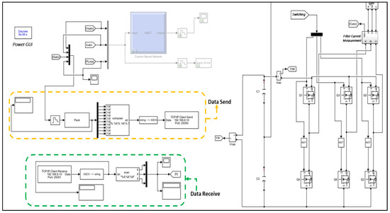
Figure 22. Data transmitting and Receiving in between SIMULINK and Raspberry PI.

Since the string data type is used with the SIMULINK environment hence, before the transmission, the data has been rendered into distinct data packets. These packets are sequentially converted to ASCII format that is acceptable for the TCP/IP port. The zero-order hold is used to synchronize the data transmission speed of SIMULINK and the microprocessor. The zero-order hold provides a mechanism for discretizing one or more signals in time or re-sampling signals at different rates [34]. As the data transmission in this methodology includes multi-rate conversion, a zero-order reserved block between fast conversion and slow conversion synchronizes the communication. The sampling rate of the zero-order hold has been set to the sampling rate at minimum data loss.

For a continuous HIL-based process HIL, Raspberry PI initially receives the input signals and further transmits the calculated 3 phase reference current signal (Ir) back to the simulated environment. The green highlighted block in Figure 22 receives the signals from the microprocessor. An identical TCP/IP port has been used for receiving and sending data. Since the received signal has to be used within the SIMULINK environment, the data type of the signal is converted from ASCII to string. The incoming data stream comprises three distinct current values for the respective three-phase currents, so the scan block transforms the incoming data stream from the TCP/IP block into 3 phase reference current (I_r).

In Figure 22, the software-based network sockets are employed to send and receive data between SIMULINK and the microprocessor. The methodology of socket programming is based on connecting two discrete nodes on a unique network to communicate with each other. One socket (node) listens on a predefined port at an IP, while the other socket responds first to form a connection loop. So, to effectively achieve this network topology, an environment based on node JavaScript (JS) is used. Node JS runs on a V8 engine; hence, this engine can efficiently handle Node-RED, which acts as a hosting service for communication between the two respective nodes (SIMULINK and Microprocessor).

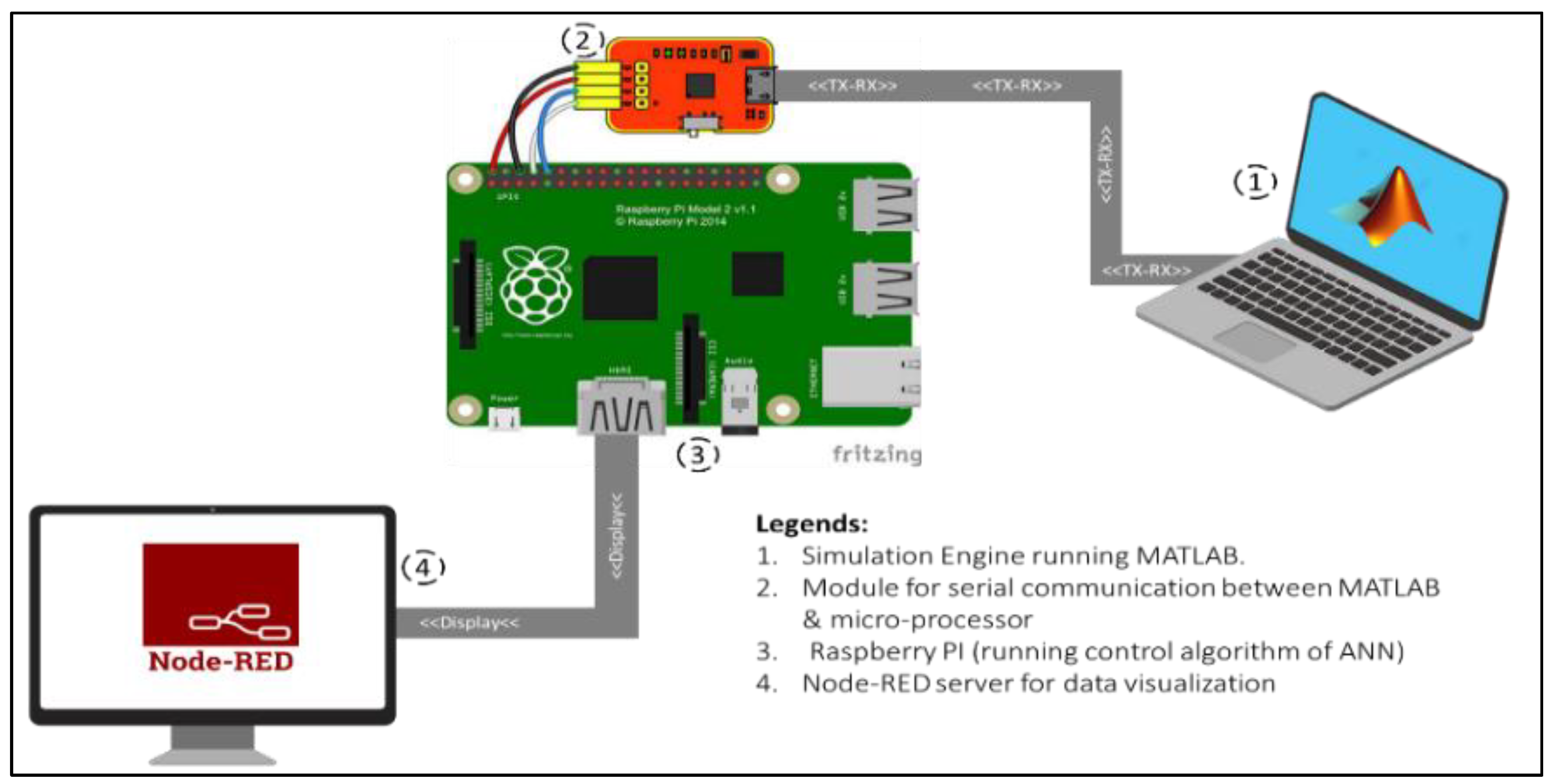
Figure 23 shows the system architecture through which Node-RED API runs in an environment based on node JS. In this research methodology, the 7 input signals for the neural network are received by the microprocessor through node-RED. In return, the microprocessor sends the reference current signals back to SIMULINK through the identical channel. Node-RED is employed to serve two applications. Firstly, it is used as a web browser-based visualization tool for real-time data receiving and sending between the microprocessor (Raspberry PI) and the simulated environment. Secondly, it is used for data rendering in the form of comma-separated values (CVS). These values are then maintained in a CVS file on a distinct URL via the Node-RED server. This URL refers to the URL of the network socket node point as the server. It can also be termed as the URL of the network socket node point in the Node-RED application. The Web socket protocol provides full-duplex communication between a client running user-defined code in a controlled environment and a remote host [35,36].

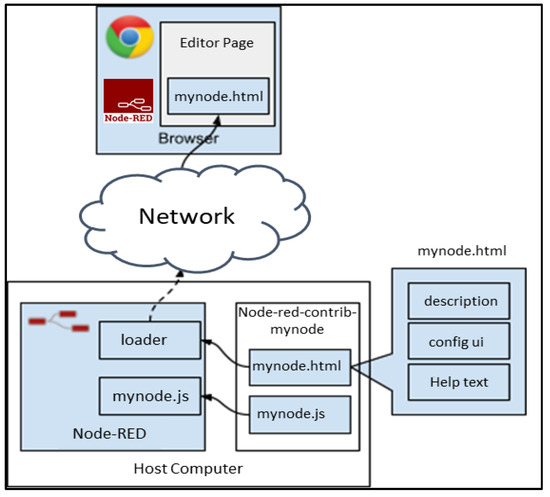
Figure 23. System Architecture for Node-RED API.

Our proposed model helps visualize data where the wireless applications are unable to work autonomously from the conventional database operations. Data access occurs concurrently from conventional centralized and/or distributed sources with wireless uses. It comprises mutually mobile queries/transactions and distribution applications. The proposed model supports visualizing all types of access, as stated in our previous work [37]. To accelerate interpretation and understanding of the proposed system model, we have recalled the various components in following operational units.

• Contents Providers (CP)s offer the data that is read/updated by users.
• Dissemination Operators (DO)s are accountable for the real data push. Moreover, CPs feed DOs together with the necessary distributed data.
• Mobile Support Stations (MSS)s are conventional that maintain bi-diirectional wireless communication along with wireless users.
• The dissemination Controller (DC) handles data to be distributed from the CPs and MSSs towards DOs.

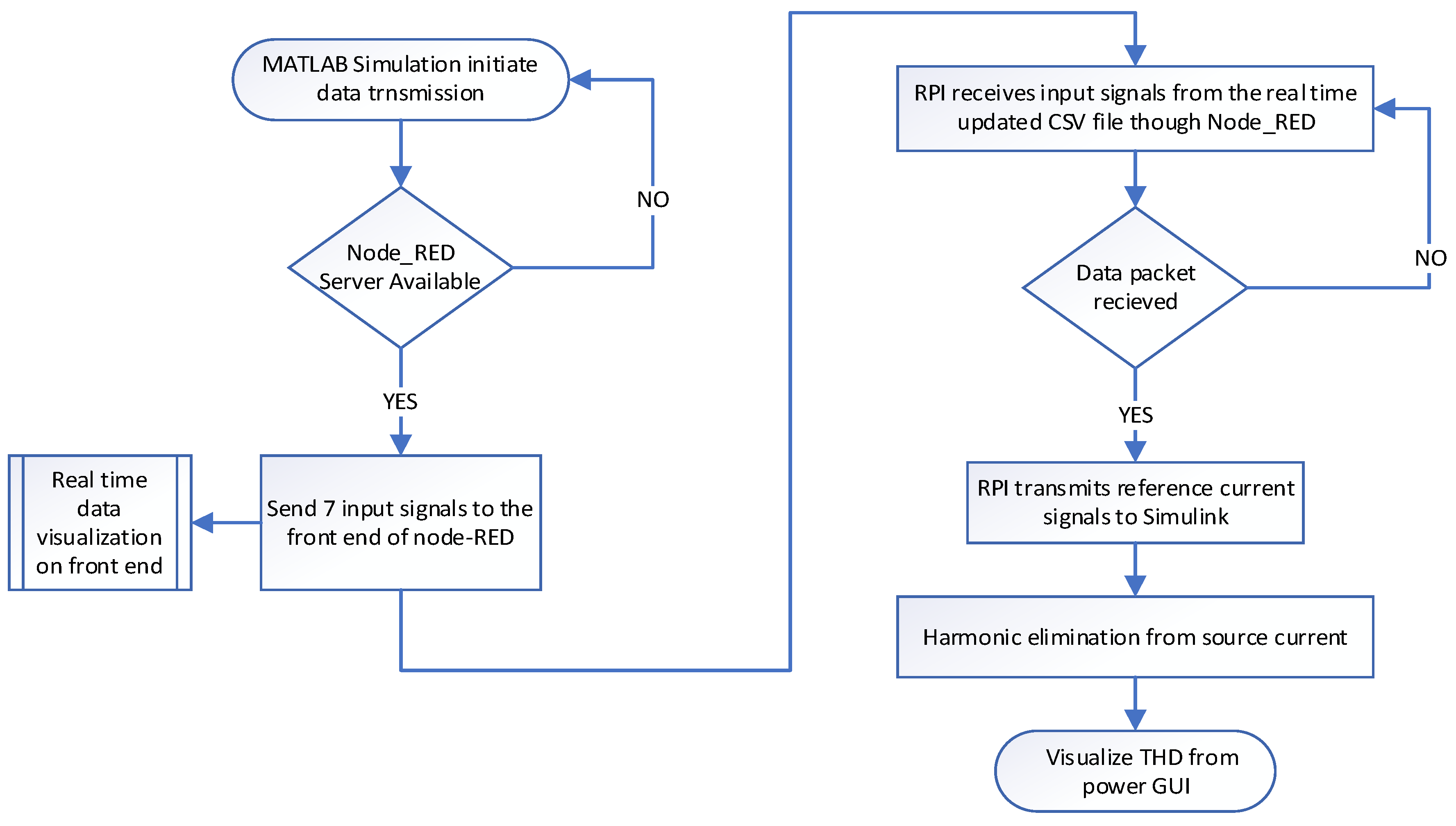
It provides durable and low-latency connections that support transactions initiated by the client and the server. Security standard employed for this purpose is commonly used in web browsers. The protocol comprises of a handshake connection establishment process and basic message framing based on TCP (Transmission Control Protocol) layering. Further, the data has been transmitted in the form of messages, and each message consists of a frame containing the data (payload) being sent [37]. On receiving a particular payload, the client ensures that the message is rebuilt correctly. Therefore, each frame has a data prefix, and the length is 4 to 12 bytes. This frame-based messaging system can significantly reduce latency. The communication uses a TCP link over a specified port suitable for non-Web Internet connections with firewalls. The flowchart in Figure 24 shows summarizes the complete implementation of HIL architecture between Raspberry PI and SIMULINK.

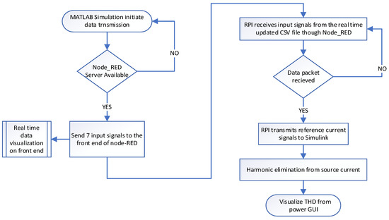
Figure 24. Flow Chart for Implementation of HIL.

3. Results and Findings

The most significant target of the research methodology is to reduce the percentage THD of source current when a variable non-linear load is operational in a HIL environment. The results obtained are distinctively divided and analyzed in following sequence.

➢

An analysis of THD with the direct introduction of non-load without a filter has been performed.

➢

In further, a simulation-based THD analysis for operational non-load with interleaving ANN-based hybrid filter has been presented.

➢

A HIL-based THD analysis for operational non-linear load with interleaving ANN-based hybrid filter is performed.

➢

Lastly, a comparative analysis has been performed.

3.1. Analysis of THD with the Direct Introduction of Non-Load without a Filter

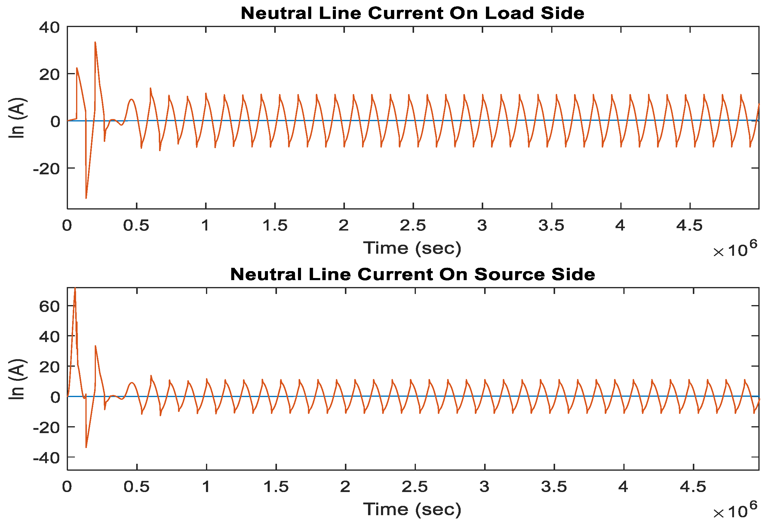
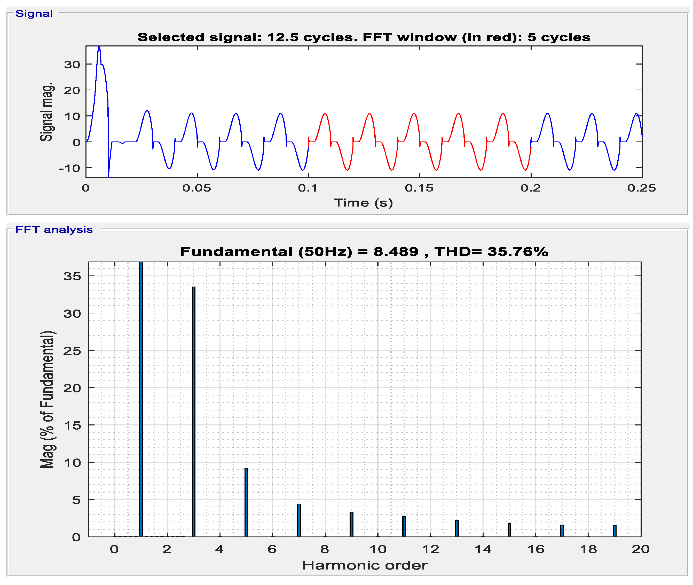
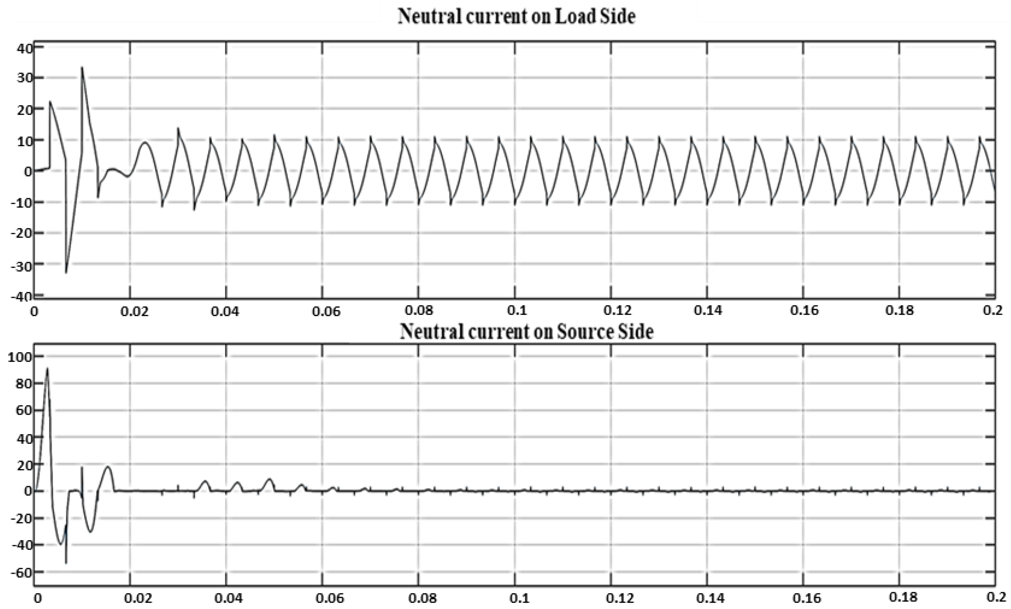
If a three-phase non-linear load is operated without applying any harmonic filter, then the current drawn by the load disturbs the balanced conditions at the bus bar of the three-phase four-wire system. As a result, this unbalanced condition introduces a current signal in the neutral line and increases the THD percentage. Figure 25 shows the current drawn from the neutral line on the source side versus the load side. As the Figure shows, the neutral line current waveform on the source side is identical to the load side. It is due to the unbalance condition introduced by the non-linear load. As a result, the source current does waveform does not remain sinusoidal, which causes intense damage to the health and eventually the working lifecycle of the industrial assets. Figure 7 and Figure 8 show the source current and voltage waveform, respectively, when a non-linear load is operated without any filter. In this scenario, when FFT analysis is done on the source current waveform, the obtained THD equals 35.76%, as shown in Figure 26.

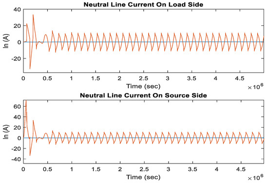
Figure 25. Neutral Line Current without Any Harmonic Filter.

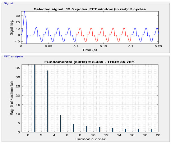
Figure 26. %THD of Source Current without Harmonic Filter.

After this analysis, the design and implementation of the hybrid harmonic filter are then performed as the next step.

3.2. Simulation-Based THD Analysis for Operational Non-Load with Interleaving ANN Based Hybrid Filter

A hybrid harmonic filter based on the control algorithm of a neural network consisting of 2 hidden layers and 20 neurons is trained to predict the reference currents based on load current, source voltage, and the DC link-level voltage. Hysteresis current-controlled loop then provides the switch angles for the IGBTs to filter the source current harmonics.

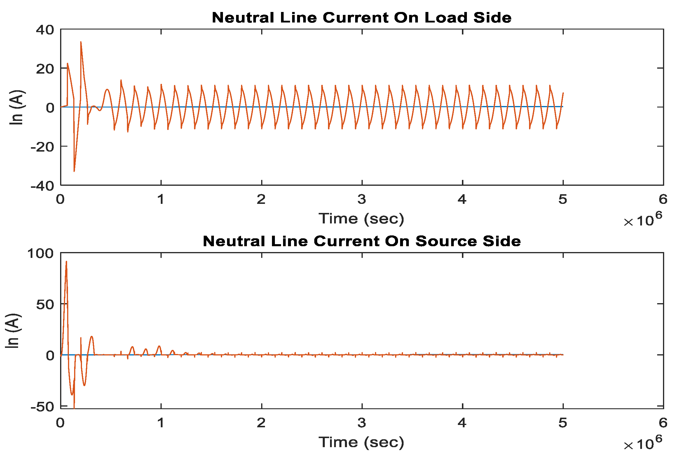
Resultantly, the neutral line current that was induced due to the application of non-linear load is reduced from an average of 12 to 0.65 Amperes. In further detail, Figure 27 depicts the current drawn from the neutral line on the source side versus the load side after applying a filter in SIMULINK. Along with reducing the neutral line current, the current drawn from the three-phase source is also transformed into a sinusoidal waveform. The presence of harmonics in the bus bar before applying the filter significantly out formed the sinusoidal waveform of the source current. It severely damages the performance of industrial assets.

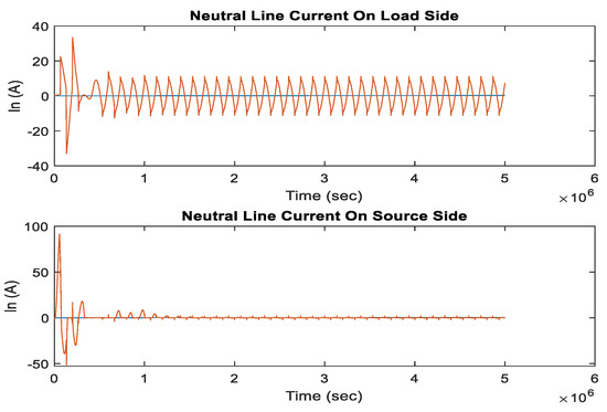
Figure 27. Neutral Line Current with Simulated ANN Based Filter.

So, after applying the designed harmonic filter, the waveform of the 3-phase source current is significantly rendered to a sinusoidal wave. Figure 28a,b shows the waveform of the source current and source voltage, respectively, when the filter is applied.

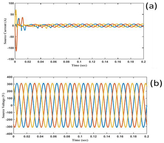
Figure 28. (a). Source Current (b). Source Voltage (with Simulated ANN Based Filter).

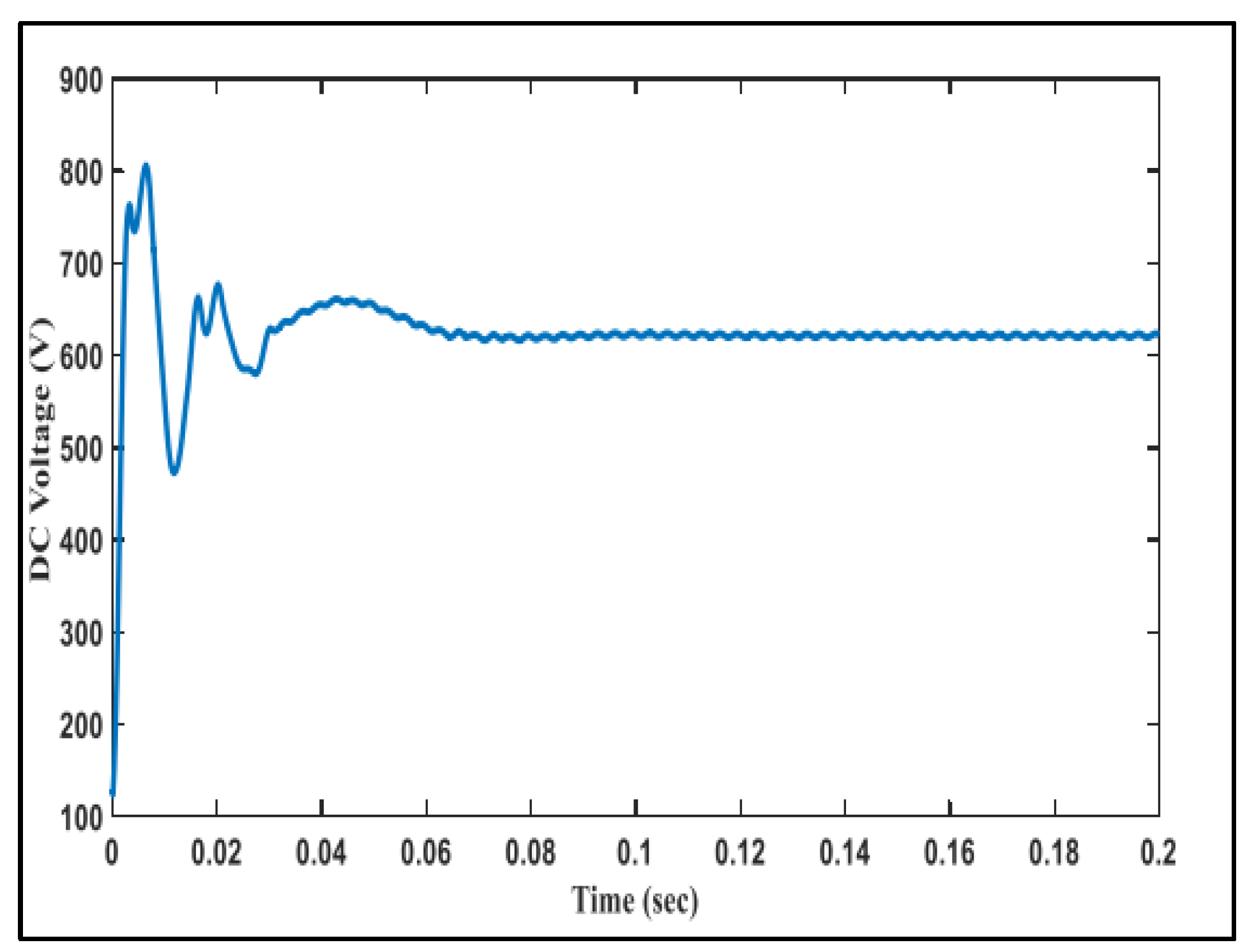
The designed hybrid filter uses IBGTs as a switching device to generate inverse harmonics further injected into the bus bar. Consequently, the voltage across the designed filter must be higher than the voltage across the bus bar to maintain an overall power. The DC link capacitors are employed to provide this consistent voltage supply. Figure 29 displays the voltage across these capacitors maintained in a steady state after the filter is applied.

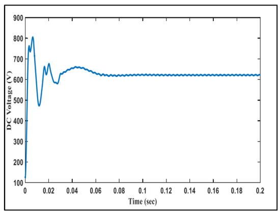
Figure 29. DC-Link Capacitor Voltage.

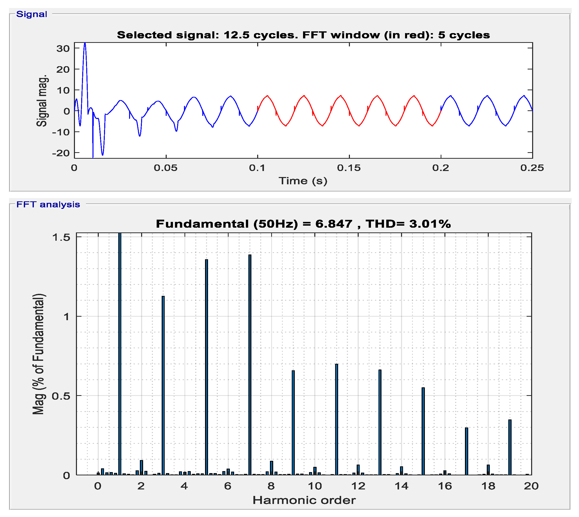
After applying the designed filter, the waveform of the source current has retained its true sinusoidal shape. Resultantly the percentage of THD is reduced from 35.76% to 3.01%. In Figure 30, the FFT analysis of source current after applying the filter is presented.

Figure 30. %THD of Source Current (Simulated ANN-based Filter).

3.3. HIL-Based THD Analysis for Operational Non-Linear Load with Interleaving ANN-Based Hybrid Filter

The first step is to program the microprocessor (Raspberry PI) to host a trained neural network that would act as a data server for the SIMULINK to implement and integrate a HIL-based topology. Tensor flow environment of python (Anaconda) programming is employed to train and deploy the neural network. With a train to test split ratio of 90/10 percent, the model is trained up to an average accuracy of 98%. Figure 31 shows the graph of training accuracy after the model is trained to 600 epochs.

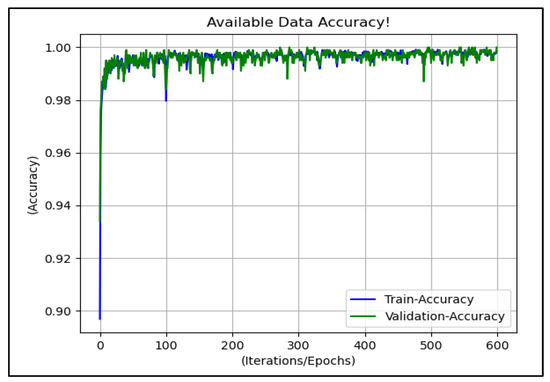
Figure 31. Training accuracy ANN model training in Raspberry PI.

After successfully training the ANN, a dataset of 10,000 samples is then fed to the trained network. Each sample consists of an array of seven inputs, i.e., three voltage signals for three-phase source voltage, three current signals for three-phase source current, and compensated signals (P_loss) to maintain the DC regulated voltage. As an output, the neural network predicts the 3-phase reference current signals shown in Figure 32. This signal would be used to provide IGBT’s switching angles through the hysteresis loop.

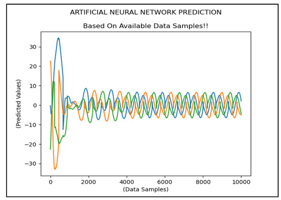
Figure 32. Output (Reference current) From ANN control algorithm.

HIL topology is significantly based on real-time data transmission and receiving between the simulated environment and the microprocessor.

Hence, the serial communication link between the two platforms is established by interfacing dedicated TCP/IP sockets. This connection is operated on a unique pre-specified port while node-red is used as a software service to host this communication channel. Furthermore, node-red is also used to design an interactive real-time data visualization tool that acts as a human-machine interface (HMI) to initiate and monitor the process of HIL. Initially, the TCP-In node sequentially receives the data set from SIMULINK. After being sorted as a symmetrical array, this data set passed through the trained ANN in the microprocessor as an input that predicts an output for the received input.

The output signal is again sent back through the TCP-Out node back to SIMULINK that completes the loop.

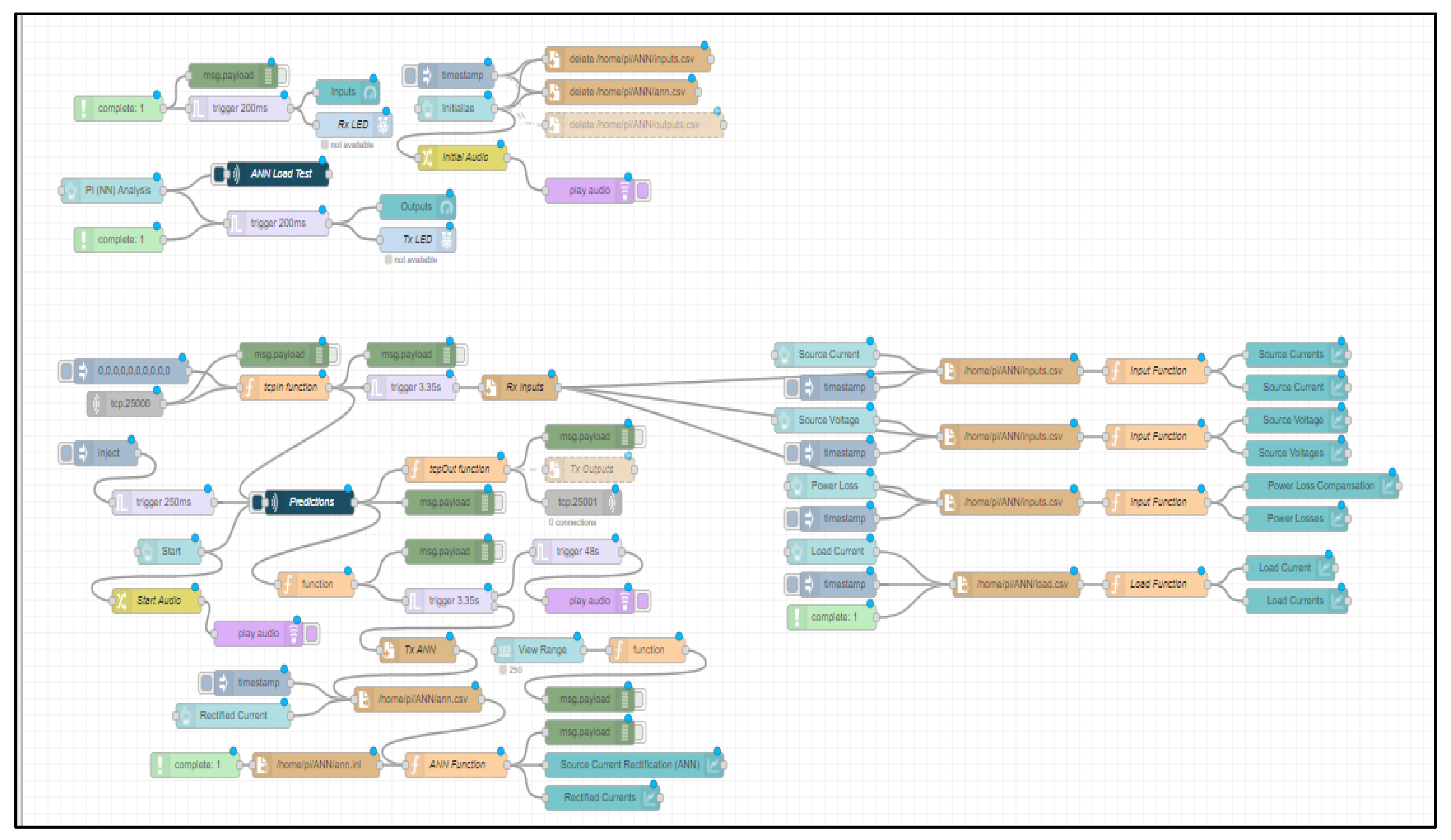
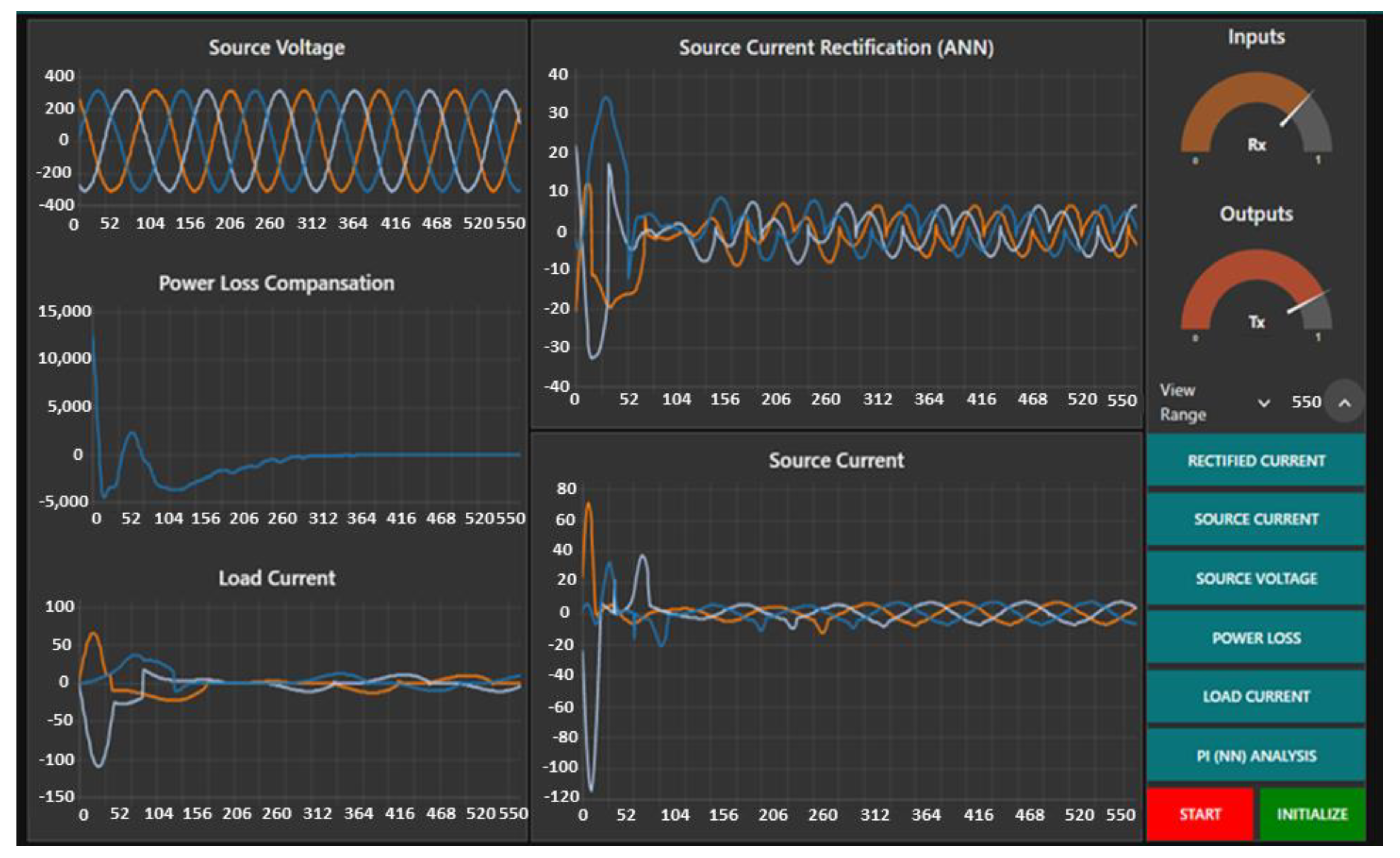
The red block shown in Figure 33 depicts the backend serial socket communication nodes. Similarly, the supervisory control of the HMI is working at the back end shown in Figure 34. The dashboard nodes used in the Figure consistently gather data from TCP send and receive blocks in a one-dimensional array and plot this data for each data sample received. Furthermore, the audio output node is programmed to indicate data initialization and the completion of every single period of data refresh rate. The following Figure 35 illustrates the front-end HMI that has been designed to operate and observe the working of HIL topology. The trends in the Figure are updated on a real-time basis on receiving a data packet. The ‘Source Current Rectification’ trend shows the output of Raspberry PI that is sent to SIMULINK.

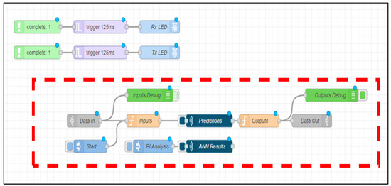
Figure 33. Backend Serial Socket Communication Nodes.

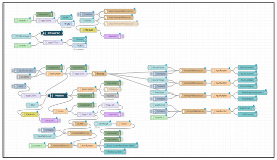
Figure 34. Backend for Supervisory Control of HMI.

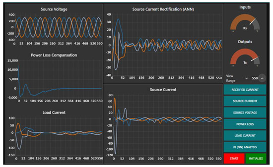
Figure 35. Node-RED Front End Dashboard.

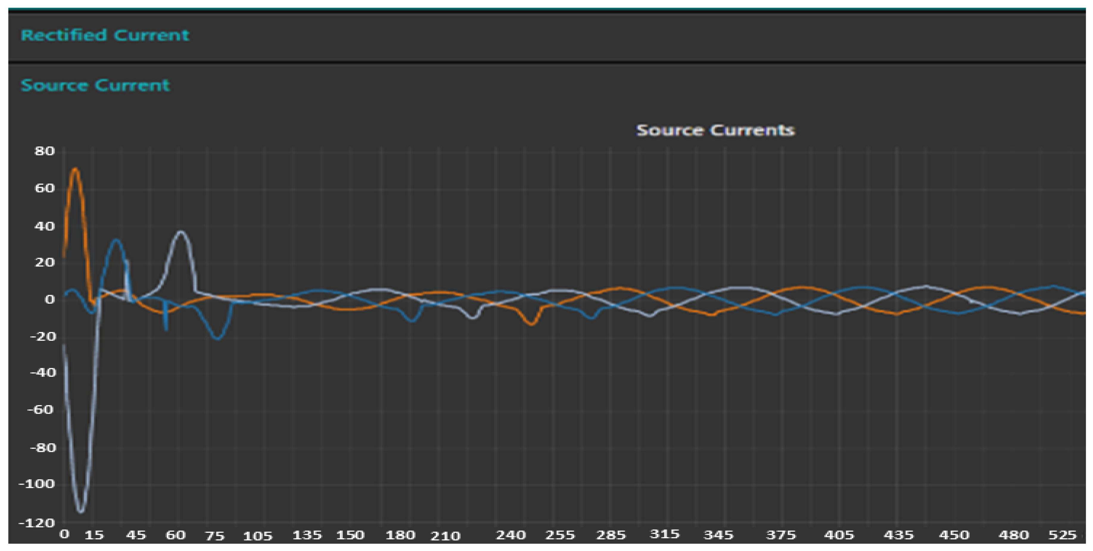
In comparison, the ‘Source Current’ trend shows the real-time current provided by the source. For individual monitoring of each parameter, a detailed chart tab is designed in which the operator can easily observe the historian trend of the specified parameter. Figure 36 shows a detailed chart Table in HIL topology, the neutral line current is reduced from an average of 12 Ampere to 0.75 after applying the harmonic filter control algorithm through Raspberry PI.

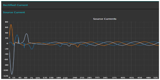
Figure 36. Historian Trends for Detailed Analysis.

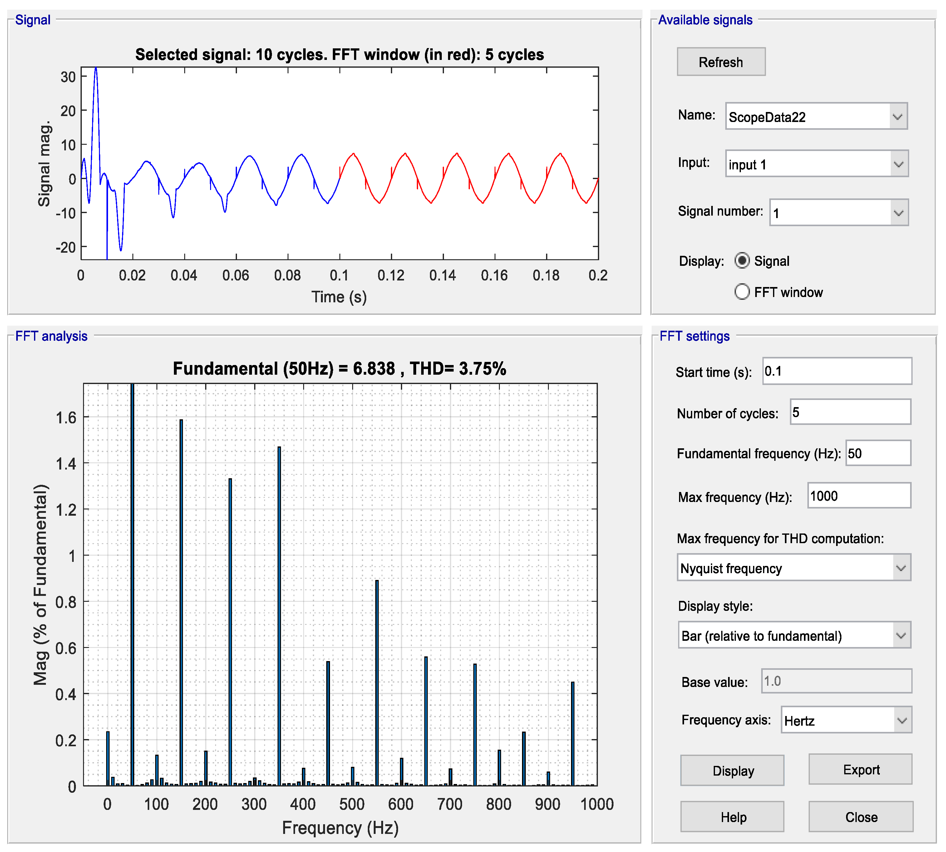
Figure 37 displays the current drawn from the neutral line on the source side versus the load side while HIL is functional. The %THD was reduced by applying a Simulation-based filter in the same way the %THD is reduced from 35.76 to 3.75 percent.

Figure 37. Neutral Line Current with ANN Based Filter In HIL Topology.

In Figure 38, the FFT analysis of source current has been displayed when the control algorithm is operated through HIL. HIL topology bears greater computational cost due to the involvement of hardware complexities, and it helps to accurately configure a physical processor to be integrated into the practical power industry.

Figure 38. %THD of Source Current with ANN Based Filter In HIL Topology.

4. Comparative Analysis

Table 4 shows a comparative analysis based on performance analysis. It is verified that integrating an external control algorithm on a physical microprocessor in HIL topology provides acceptable results by international standards. Hence, the percentage THD and stability time achieved in the proposed methodology with the existing techniques in the available literature. Table 5 shows the comparison of proposed methodology with existing literature

Table 4. Comparative Analysis.

	Parameters	THD (%)	Neutral Wire Current (Amp)	Stability Time (s)	DC Voltage Fluctuations (Volt)
Control Techniques
Pq0 theory Implemented in SIMULINK		3.28	0.9	0.06	3.891
ANN Based Filter Implemented In SIMULINK		3.01	0.67	0.06	1.794
Pq0 theory based Filter Implemented In Raspberry PI		3.57	0.68	0.06	2.012
ANN Based Filter Implemented In Raspberry PI		3.75	0.75	0.06	2.314

Table 5. Comparison of Proposed Methodology with Existing Literature.

	Parameters	HIL Based Approach	% THD	Stability Time (s)
Research Work
Proposed Methodology		YES	3.75	0.06
[11]		YES	3.82	0.11
[22]		NO	8.77	0.1
[28]		NO	3.25	0.05
[31]		NO	2.39	2.1
[33]		NO	3.59	0.14
[38]		NO	7.01	0.08

5. Conclusions

Conventionally, most industrial loads vary and are non-linear, introducing harmful harmonics in the power distribution system. So, an ANN-based hybrid shunt active harmonic power filter (HSAHPF) design is proposed to eliminate the effects of the generated harmonics. This design works on HIL topology using Raspberry PI as a central control unit for an ANN-based algorithm. Moreover, we have used MATLAB/SIMULINK as a test environment for the algorithm. In the presented environment, a simulated load and power supply are employed to power up and observe the working of the designed filter while the control parameters are transmitted via serial TCP/IP protocol.

Additionally, the network has been trained on the principles of backpropagation that uses the tensor flow library of python. A training accuracy of 99.9% has been achieved using ADAM optimizer for specified data set of Pq0 theory. The experimental results of the proposed implementation validate the design of the filter. It can be observed from the presented statistics that the designed filter is proficient for THD reduction as the value has been reduced from 35.76% to 3.75% that meets the standard limits of IEEE. Conclusively, comparative analysis has observed that the realized values through HIL configuration are almost identical to the results of the simulation-based control architecture.

The targeted beneficiaries of this research are the production industries where heavy electrical loads are being operated because further development on this topic resides on the application of a designed controller with a physical power source and non-linear loads. In the current state, this research methodology is a prototype dependent upon the simulated environment’s existence. So, research can be done on this topic to configuring the proposed algorithm with the industrial controllers commonly termed as Programmable Logic Controllers (PLCs). Furthermore, a hardware-based optically isolated voltage source inverter can be customized to integrate the programmed controller. It would therefore provide a compact hardware solution without the dependency upon simulations.

References

- Zechariah, S.S. Hybrid Harmonic Filter for Electrical Power Systems. Ph.D. Dissertation, Tunku Abdul Rahman University College, Kuala Lumpur, Malaysia, 2019. [Google Scholar]
- Das, J. Passive Filters—Potentialities and Limitations. IEEE Trans. Ind. Appl. 2004, 40, 232–241. [Google Scholar] [CrossRef]
- Wang, Y.; Yong, J.; Sun, Y.; Xu, W.; Wong, D. Characteristics of Harmonic Distortions in Residential Distribution Systems. IEEE Trans. Power Deliv. 2017, 32, 1495–1504. [Google Scholar] [CrossRef]
- Haghdar, K.; Heidar, A.S. Selective harmonic elimination with optimal DC sources in multilevel inverters using generalized pattern search. IEEE Trans. Ind. Inform. 2018, 14, 3124–3131. [Google Scholar] [CrossRef]
- Dahidah, M.S.A.; Konstantinou, G.; Agelidis, V.G. A Review of Multilevel Selective Harmonic Elimination PWM: Formulations, Solving Algorithms, Implementation and Applications. IEEE Trans. Power Electron. 2015, 30, 4091–4106. [Google Scholar] [CrossRef]
- Singh, H.; Kour, M.; Thanki, D.V.; Kumar, P. A Review on Shunt Active Power Filter Control Strategies. Int. J. Eng. Technol. 2018, 7, 121–125. [Google Scholar] [CrossRef]
- Albatsh, F.M.; Hassan, M.; Ahmad, S.; Mekhilef, S.; Mokhlis, H. D-Q model of Fuzzy based UPFC to control power flow in transmission network. In Proceedings of the 7th IET International Conference on Power Electronics, Machines and Drives (PEMD 2014), Manchester, UK, 8–10 April 2014; pp. 5–13. [Google Scholar]
- Diab, M.; El-Habrouk, M.; Abdelhamid, T.H.; Deghedie, S. Survey of Active Power Filters Configurations. In Proceedings of the 2018 IEEE International Conference on System, Computation, Automation and Networking (ICSCA), Pondicherry, India, 6–7 July 2018; pp. 1–14. [Google Scholar]
- Kalair, A.; Abas, N.; Kalair, A.R.; Saleem, Z.; Khan, N. Review of harmonic analysis, modeling and mitigation techniques. Renew. Sustain. Energy Rev. 2017, 78, 1152–1187. [Google Scholar] [CrossRef]
- Lin, X.; Xia Hou, K.; Liu, Y.; Wu, Q.H. Design and Hardware-in-the-Loop Experiment of Multiloop Adaptive Control for DFIG-WT. IEEE Trans. Ind. Electron. 2018, 65, 7049–7059. [Google Scholar] [CrossRef]
- Noshahr, J.; Mehdi, B.; Mostafa, K. The Estimation of the Influence of Each Harmonic Component in Load Unbalance of Distribution Transformers in Harmonic Loading Condition. In Proceedings of the 2019 IEEE International Conference on Environment and Electrical Engineering and 2019 IEEE Industrial and Commercial Power Systems Europe (EEEIC/I&CPS Europe), Genova, Italy, 11–14 June 2019; pp. 1–6. [Google Scholar]
- Soomro, D.M.; Soo, C.C.; Zubair, A.M.; Mohammad, A.U.; Farhan, A. Per-formance of shunt active power filter based on instantaneous reactive power control theory for single-phase system. Int. J. Renew. Energy Res. (IJRER) 2017, 7, 1741–1751. [Google Scholar]
- Gali, V.; Nitin, G.; Gupta, R.A. Enhanced Particle Swarm Optimization Technique for Interleaved Inverter Tied Shunt Active Power Filter. In Soft Computing for Problem Solving; Springer: Singapore, 2019; pp. 571–583. [Google Scholar]
- Madhu, M.B.; Mn, D.; Bm, R. Design of shunt hybrid active power filter (SHAPF) to reduce harmonics in AC side due to Non-linear loads. Int. J. Power Electron. Drive Syst. (IJPEDS) 2018, 9, 1926–1936. [Google Scholar] [CrossRef]
- Fang, Y.; Fei, J.; Ma, K. Model reference adaptive sliding mode control using RBF neural network for active power filter. Int. J. Electr. Power Energy Syst. 2015, 73, 249–258. [Google Scholar] [CrossRef]
- Agrawal, S.; Prakash, K.; Palwalia, D.K. Artificial neural network based three phase shunt active power filter. In Proceedings of the 2016 IEEE 7th Power India International Conference (PIICON), Bikaner, India, 25–27 November 2016; pp. 1–6. [Google Scholar]
- Singh, S.K.; Arup, K.G.; Nidul, S. Power system harmonic parameter estimation using bi-linear recursive least square (BRLS) algorithm. Int. J. Electr. Power Energy Syst. 2015, 67, 1–10. [Google Scholar] [CrossRef]
- Li, H.; Gole, A.M.; Ho, C.N.M. Controller Implementation and Performance Evaluation of a High Power Three-Phase Active Power Filter using Controller Hardware-in-the-Loop Simulation. In Proceedings of the 2018 IEEE Electrical Power and Energy Conference (EPEC), Toronto, ON, Canada, 10–11 October 2018; pp. 1–6. [Google Scholar]
- Fabricio, E.L.L.; Junior, S.C.S.; Jacobina, C.B.; Correa, M.B.D.R. Analysis of Main Topologies of Shunt Active Power Filters Applied to Four-Wire Systems. IEEE Trans. Power Electron. 2018, 33, 2100–2112. [Google Scholar] [CrossRef]
- Khan, A.; Hussain, M.; Javed, Y.; Arshad, J.; Rehman, A.; Khan, R.; Bajaj, M.; Kaabar, M.K.A. Hardware-in-the-Loop Implementation and Performance Evaluation of Three-phase Hybrid Shunt Active Power Filter for Power Quality Improvement. Math. Probl. Eng. 2021, 2021, 1–23. [Google Scholar] [CrossRef]
- Asif, R.M.; Rehman, A.U.; Rehman, S.U.; Arshad, J.; Hamid, J.; Sadiq, M.T.; Tahir, S. Design and analysis of robust fuzzy logic maximum power point tracking based isolated photovoltaic energy system. Eng. Rep. 2020, 2, 12234. [Google Scholar] [CrossRef]
- Manoharsha, M.; Babu, B.; Veeresham, K.; Kapoor, R. ANN based Selective Harmonic Elimination for Cascaded H-Brdige Multilevel Inverter. In Proceedings of the 2021 7th International Conference on Electrical Energy Systems (ICEES), Chennai, India, 11–13 February 2021; pp. 183–188. [Google Scholar]
- Ata, R. RETRACTED: Artificial neural networks applications in wind energy systems: A review. Renew. Sustain. Energy Rev. 2015, 49, 534–562. [Google Scholar] [CrossRef]
- Bouyakoub, I.; Taleb, R.; Mellah, H.; Zerglaine, A. Implementation of space vector modulation for two level Three-phase inverter using dSPACE DS1104. Indones. J. Electr. Eng. Comput. Sci. 2020, 20, 744–751. [Google Scholar] [CrossRef]
- Herman, L.; Bozicek, A.; Blažič, B.; Papic, I. Real-time simulations of a parallel hybrid active filter with hardware-in-the-loop. In Proceedings of the 2014 16th International Conference on Harmonics and Quality of Power (ICHQP), Bucharest, Romania, 25–28 May 2014; pp. 576–580. [Google Scholar]
- Zou, Z.-X.; Zhou, K.; Wang, Z.; Cheng, M. Frequency-Adaptive Fractional-Order Repetitive Control of Shunt Active Power Filters. IEEE Trans. Ind. Electron. 2015, 62, 1659–1668. [Google Scholar] [CrossRef]
- Chawda, G.S.; Shaik, A.G. Performance Evaluation of Adaline Controlled Dstatcom for Multifarious Load in Weak AC Grid. In Proceedings of the 2019 IEEE PES GTD Grand International Conference and Exposition Asia (GTD Asia), Bangkok, Thailand, 19–23 March 2019; pp. 356–361. [Google Scholar]
- Zellouma, L.; Boualaga, R.; Abdelbasset, K.; Amar, B.; Benkhoris, M.F. Simulation and real time im-plementation of three phase four wire shunt active power filter based on sliding mode controller. Rev. Roum. Des. Sci. Technol. Ser. Electrotech. Energy 2018, 63, 77–82. [Google Scholar]
- Mikkili, S.; Panda, A.K. Instantaneous Active and Reactive Power and Current Strategies for Current harmonics cancellation in 3-ph 4wire SHAF With both PI and Fuzzy Controllers. Energy Power Eng. 2011, 3, 285–298. [Google Scholar] [CrossRef] [Green Version]
- Li, D.; Wang, T.; Pan, W.; Ding, X.; Gong, J. A comprehensive review of improving power quality using active power filters. Electr. Power Syst. Res. 2021, 199, 107389. [Google Scholar] [CrossRef]
- Karthikeyan, M.; Sharmilee, K.; Balasubramaniam, P.; Prakash, N.; Babu, M.R.; Subramaniyaswamy, V.; Sudhakar, S. Design and implementation of ANN-based SAPF approach for current harmonics mitigation in industrial power systems. Microprocess. Microsyst. 2020, 77, 103194. [Google Scholar] [CrossRef]
- Siregar, S.P.; Wanto, A. Analysis of Artificial Neural Network Accuracy Using Backpropagation Algorithm In Predicting Process (Forecasting). Int. J. Inf. Syst. Technol. 2017, 1, 34–42. [Google Scholar] [CrossRef] [Green Version]
- Moeini, A.; Dabbaghjamanesh, M.; Kimball, J.W.; Zhang, J. Artificial Neural Networks for Asymmetric Selective Harmonic Current Mitigation-PWM in Active Power Filters to Meet Power Quality Standards. IEEE Trans. Ind. Appl. 2020, 1. [Google Scholar] [CrossRef]
- Kim, S.-B.; Sok, V.; Kang, S.-H.; Lee, N.-H.; Nam, S.-R.; Kim, S.; Kang, L.N. A Study on Deep Neural Network-Based DC Offset Removal for Phase Estimation in Power Systems. Energies 2019, 12, 1619. [Google Scholar] [CrossRef] [Green Version]
- Singh, D.; Singh, M.; Hakimjon, Z. Requirements of MATLAB/Simulink for signals. In Signal Processing Applications Using Multidimensional Polynomial Splines; Springer: Singapore, 2019; pp. 47–54. [Google Scholar]
- Toc, S.-I.; Korodi, A. Modbus-OPC UA Wrapper Using Node-RED and IoT-2040 with Application in the Water Industry. In Proceedings of the 2018 IEEE 16th International Symposium on Intelligent Systems and Informatics (SISY), Subotica, Serbia, 13–15 September 2018; pp. 99–104. [Google Scholar]
- Al Mogren, A.S. The integration of telecommunication and dissemination networks. Int. J. Commun. Netw. Distrib. Syst. 2010, 4, 331. [Google Scholar] [CrossRef]
- Yang, K.; Hao, J.; Wang, Y. Switching angles generation for selective harmonic elimination by using artificial neural networks and quasi-newton algorithm. In Proceedings of the 2016 IEEE Energy Conversion Congress and Exposition (ECCE), Milwaukee, WI, USA, 18–22 September 2016; pp. 1–5. [Google Scholar]
Publisher’s Note: MDPI stays neutral with regard to jurisdictional claims in published maps and institutional affiliations. |
© 2021 by the authors. Licensee MDPI, Basel, Switzerland. This article is an open access article distributed under the terms and conditions of the Creative Commons Attribution (CC BY) license (https://creativecommons.org/licenses/by/4.0/).