Use of Learning Mechanisms to Improve the Condition Monitoring of Wind Turbine Generators: A Review

Abstract

The main goal of this paper is to review and evaluate how we can take advantage of state-of-the-art machine learning techniques and apply them in wind energy operation conditions monitoring and fault diagnosis, boosting wind turbines’ availability. To accomplish this, we focus our work on analysing the current techniques in predictive maintenance, which are aimed at acting before a major failure occurs using condition monitoring. In particular, we start framing the predictive maintenance problem as an ML problem to detect patterns that indicate a fault on turbine generators. Then, we extend the problem to detect future faults. Therefore, this review will consist of analysing techniques to tackle the challenges of each machine learning stage, such as data pre-processing, feature engineering, and the selection of the best-suited model. By using specific evaluation metrics, the expected final result of using these techniques will be an improvement in the early prediction of a future fault. This improvement will have an increase in the availability of the turbine, and therefore in energy production.

1. Introduction

As a consequence of increasing climate change awareness, research on topics such as renewable energy are of extreme importance. An event that played a significant role in rapidly finding practical solutions to stop those changes was the Paris Agreement. The long term goal of that agreement was to limit temperature rises; therefore, countries needed to adapt their current practices to reduce carbon emissions (https://unfccc.int/process-and-meetings/the-paris-agreement/the-paris-agreement (accessed on 17 October 2021)).

Since the power sector is one of the main contributors to global greenhouse gas emissions (https://www.c2es.org/content/international-emissions (accessed on 17 October 2021)), new technologies for cleaner energy production have been developed to replace conventional production (e.g., production based on fossil fuels) [1]. To create incentives for developers to invest in cleaner energy technologies, countries (e.g., China, Russia, India, Japan, Brazil, and European countries) have proposed national action plans. By analysing those national plans, we can observe that some of them highlighted that wind energy can have a major contribution as a zero-emission energy source. Consequently, the “European Green Deal” (https://ec.europa.eu/info/strategy/priorities-2019-2024/european-green-deal_en (accessed on 17 October 2021)) emerged as an extension at the continent level. The main objective of the EU Green Deal is for the EU to become the first climate-neutral continent by 2050 [2]. Regarding the energy sector, these are some of the main goals: build interconnected energy systems and better integrated grids to support renewable energy sources, decarbonize the gas sector, promote smart integration across sectors, and develop the full potential of Europe’s off-shore wind energy [3].

As a consequence of the previous initiative, the future of energy will profoundly depend on renewable energies, such as wind and photovoltaic energy. Therefore, this review will focus on wind technology due to its increasing importance in the last few years. The cumulative installed capacity of both off- and on-shore wind energy has been growing, with global yearly new installations rounding 50 GW. In 2020, it even surpassed 90 GW, a 53% growth compared to 2019, bringing the total installed capacity to 743 GW. (https://gwec.net/wp-content/uploads/2021/03/GWEC-Global-Wind-Report-2021.pdf (accessed on 17 October 2021)) According to [4], the global installed capacity of on-shore wind power would increase (taking 2018 as reference) three-fold by 2030 (to 1787 GW) and ten-fold by 2050 (to 5044 GW). Concerning off-shore installations, the predictions are similar, with the global off-shore wind capacity rising 228 GW in 2030 and nearly 1000 GW in 2050, compared with the 23 GW installed in 2018 [4].

Wind farms are usually connected in remote areas far from the big cities and large consumption centers. A key reason for energy producers to select remote locations, such as off-shore, is the better wind conditions. Near big cities, wind suffers a lot of interference, which is not ideal for wind generators. Adding to that, we avoid visual impact and land use issues. However, some disadvantages arise from this location decision, such as connecting the wind farm to the transmission networks, transportation and installation of giant turbines, and operation and maintenance (OM) costs. Nevertheless, knowing that previously mentioned benefits might reveal that it is worth investing in transmission infrastructure to access them [5]. To reinforce the need for OM, wind farms in general and wind turbines in particular are exposed to unpredictable and harsh weather conditions, which result in highly variable and volatile operational conditions, leading to intense mechanical stress (the description of more specific problems of wind turbine generators is covered in Section 2.1).

Since it is complicated to reduce the initial costs of transportation and installation, most of the research has focused on maintenance, more specifically in the use of condition monitoring (CM). CM consists of monitoring the components of a wind turbine to identify changes in operation that can be indicative of a developing fault and preventing it through maintenance. CM increases the availability of the wind farm and, as a result, the production of electricity, decreasing the global cost of the project. There are different types of maintenance, as we will see in Section 2.1. However, the one that uses CM is called predictive maintenance. This type of maintenance has two main advantages: (i) increasing the availability of wind generators and (ii) reducing the costs of wind farms maintenance by reducing or delaying corrective maintenance actions. The first advantage plays quite an important role. For example, a wind turbine (WT) of 2.0 MW can generate 48 MWh during a day (in maximum) and generate a revenue of 3600€ when considering an average FiT (feed-in tariff) (Policy mechanism designed to accelerate investment in renewable energy technologies by offering long-term contracts to renewable energy producers) of 75 €/MWh.

Until recently, monitoring has only relied on manual and straightforward analyses of specific measurements and aspects of operation [6]. However, this type of analysis is inefficient when detecting electrical (including power electronics), mechanical, and hydraulic problems. To date, developments in sensors and signal processing systems have improved the quality and quantity of data obtained [7]. These data, when combined with machine learning (ML) and big data analysis and management, have opened up a new world of possibilities for reliable, cost-effective, and more accurate decision-making in CM.

The key goal of this review is to take advantage of these previously mentioned advances, applying them in wind turbines generator condition monitoring. In particular, we can frame the predictive maintenance problem as an ML problem, finding the best tools and methods for each one of the sub-tasks in Figure 1. Using real data obtained from SCADA (Supervisory Control And Data Acquisition) systems, the first task, Data acquisition and pre-processing, will deal with the variety and quantity of data obtained. In other words, this task does the necessary pre-processing of the data to remove outliers and treat missing values. The second task, feature selection, selects the features that better represent the patterns in the data, removing unnecessary noise. According to the obtained data, the third stage aims to select the best ML model to detect and predict faults. Finally, in the validation stage, we assess the accuracy of the ML model on classifying new data as representative of a failure in the turbine or not.

The main difference between this review and the existing ones [8,9,10,11,12,13] is that it tries to gather the strengths of each article from a ML point of view. It will not be a general review on wind turbine CM, but a tailored version comprising only ML approaches. Moreover, it will be organized as an ML problem, focusing on each of the stages mentioned in Figure 1. In addition, we will trim the review to turbine generator problems. We will start by giving a broader view on fault detection through models that can predict production related problems, models that focus on multi-target prediction, others that use transfer learning and ending with federated deep learning. Subsequently, by focusing on generator faults, we review the prediction of more specific problems, giving additional information regarding that fault that can help to prevent it. In conclusion, the present review discusses the most important ML techniques used in condition monitoring, considering a structured methodology used in data analytics. Therefore, this review will help to structure the implementation of each of the ML phases on turbine generators CM.

The remainder of this paper is organized as follows. Section 2 presents a brief background on CM of wind turbines and a state-of-the-art review on machine learning. Section 3 provides the relevant related work on each of the machine learning phases. Finally, in Section 4, we present a discussion of measures to validate the quality of the proposed models, and Section 5 summarizes the findings with conclusions, and discusses future work.

2. Background

To better understand the following sections, in Section 2.1, we present an introduction regarding condition monitoring of wind turbines. Secondly, in Section 2.2, we review state-of-the-art machine learning to help substantiate the critical analysis. Additional information on how a wind turbine works or on its key components can be found in several references in the literature, such as in Pao et al. [14].

2.1. Condition Monitoring of Wind Turbines

This section shows how to apply CM on wind turbines and presents the different approaches.

The maintenance cost of components of a wind turbine strongly depends on how we address the problem. Reactive maintenance consists of only replacing the component when it fails and does not use CM, which is the most expensive approach. Small wind farms typically rely on this approach because they do not have a permanent maintenance team. On the other hand, predictive maintenance, through CM, enables an operator to know when to replace a component before a fault occurs. This approach prevents major failures, decreasing the costs and saving up to 20–25% of maintenance costs of wind turbines [15]. Consequently leading us to another aspect: how do we choose the turbine’s element(s) to be monitored? A good strategy would be to prioritize components that are more likely to fail or lead to long down periods. Components such as the rotor and transmission system tend to have a higher rate of failure [16]. Generators tend to have a higher rate of failure in off-shore wind turbines than in on-shore ones [8].

There are also various methods of performing CM, ones more intrusive (wear out the component) than others, including acoustic emission measurement, power quality (harmonics measurements) and temperature monitoring, oil debris monitoring, and vibration analysis [17].

Finally, we can use CM for diagnosis, i.e., fault detection in real-time, or we can use it for prognosis, i.e., fault prediction. For instance, for generator faults, we have some common problems as wearing, electrical problems, rotor asymmetries, overheating and overspeed. Some of the respective current CM techniques are temperature, vibration, torque, current, voltage and power signal analysis, performance monitoring and thermography [9].

Tchakoua et al. [9] discussed some of the limitations and possible improvements on current CM techniques:

• Select a cost-effective monitoring method;
• Automate the diagnosis made by experts;
• Focus on developing precise prognostic techniques;
• Optimize the use of SCADA data for automatic monitoring;
• Improve sensors making them wireless, being easy to place in locations hard to reach;
• Use signal processing techniques for feature extraction useful for predicting WT’s components health.

Although these future research areas may appear challenging to address, they also represent great opportunities for CM to boost the wind industry’s success by reducing the cost of energy (COE) and increasing its competitiveness.

2.2. State-of-the-Art Machine Learning

To better understand how machine learning can be helpful, we present a brief introduction to the subject and the state-of-the-art regarding condition monitoring to address fault detection and diagnosis issues.

Recently, the field of condition monitoring has moved from the use of conventional techniques to artificial intelligence (AI) techniques [18]. The conventional methods consisted of sensing technologies or analysing physical quantities, as seen in the previous section, having the major problem of needing an expert to do the diagnosis. AI tries to automate this diagnosis, removing human error while handling more data in real-time. AI through machine learning techniques has been widely used to improve the accuracy and efficiency of fault detection and diagnosis, as we will see in Section 3.

ML models can follow two different approaches: supervised learning that predicts an output variable using labelled input data, or unsupervised learning that can learn from unlabelled data. In addition, for supervised learning, we have two different models; one predicts a numeric variable (regression) and the other a categorical variable (classifiers) [19].

The ML model selection phase is the most important as it is the main tool that learns from past data and generalizes into the future. For example, neural networks (NNs) and support vector machines (SVMs) are two popular models that have been used in ML for diagnostics and prognostics [8].

A NN is the adaptation of the learning ability of neurons in the brain to a computational architecture. We arrange NN in layers, and each layer is composed of a set of artificial neurons. Each neuron receives an input signal, manipulates it, and then the output is forwarded to the next layer of neurons [20]. NNs have been evolving rapidly over time. In the beginning, these models could only solve linear classification problems, which in the majority of the cases, we cannot apply in fault detection. Then, NNs evolved to multi-layered architecture that could solve non-linear problems, such as the feed-forward multi-layered method [21,22], in which no feedback from the previous signal is provided to the next. Another example is recurrent neural networks (RNNs) [23], which have feedback connections, and past signals are used to identify new features. Long short-term memory networks (LSTM) [24,25] are a type of RNNs, but instead of taking as input a single data point, they can process entire sequences of data.

In this review, self-organizing maps (SOMs), another type of NN, are also considered [21]. SOMs are trained using unsupervised learning. They produce a low-dimensional (usually two-dimensional) and discretized representation of the input training space. For this reason, we call it a map, and we typically use this method for dimensionality reduction. SOMs differ from other NNs, as they apply competitive learning as opposed to error-correction learning.

We also present two more types of NNs used for fault detection: generalized mapping regressor (GMR) and general regression neural network (GRNN) [22]. GMR is a self-supervised incremental neural network. This method can approximate every multidimensional function or relation that presents any discontinuity. The goal of GMR is to turn the function approximation problem into an unsupervised problem capable of pattern recognition. Therefore, it uses a coarse-to-fine strategy mapping. GRNN is an incremental self-organizing competitive neural network. GRNNs belong to the family of kernel neural networks. The typical GRNN training procedure minimizes the mean square error (MSE) and uses a cross-validation (leave-one-out) approach. Finally, adaptive neuro-fuzzy inference system (ANFIS) is also an important type of NN in the field of condition monitoring [23,26]. ANFIS integrates both neural networks and fuzzy logic principles. Therefore, it captures the strengths of both in a single framework. Its inference system is based on a set of fuzzy IF-THEN rules, with the learning ability to approximate non-linear functions.

The availability of larger datasets, variety of activation functions, and stronger computational power made it possible to add hidden layers (layers that allow a NN to filter/transform the data). This approach is called deep learning, and has started to be used in the wind energy field. NNs can be used for a variety of tasks, such as control (e.g., wind turbine power control) and fault diagnosis and forecasting (e.g., wind speed forecasting) [27,28], as we will describe in Section 3.

As for SVMs, they are often used in fault detection [23,29,30,31]. SVMs work by finding decision boundary hyperplanes that best separate classes samples; more specifically, the ones that leave the widest possible margin to the samples closest to the hyperplanes. They evolved from performing only linear classification or regression to non-linear problems by adding polynomial features created from existing ones. This method makes the problem linearly separable in a higher-dimensional space. They have recently gained significant importance because of their superior ability to accurately represent the relationship between the input and the output from a small amount of training information.

3. Machine Learning Techniques Applied to Condition Monitoring

In the previous section, we ended by summarizing the evolution of the use of ML in CM. In this section, we will cover the recent research on the subject of this review, including possible limitations and suggested improvements.

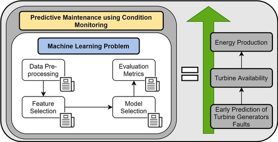
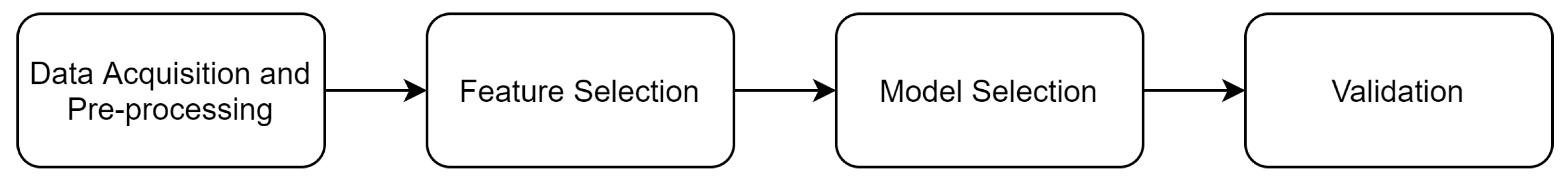
Before using ML methods, we typically use pre-processing techniques on the data, such as feature selection. Hence, it might be helpful to first look into work related to those initial tasks. After that, we will cover models for specific tasks. In Section 3.3, we start with models for more general issues, such as “Turbine performance assessment” and “Power curve monitoring”, that are not specific to a turbine component. Moving to “Multi-target normal behaviour models”, where we cover models that can be used for establishing the normal behaviour of multiple turbine components. In “Transfer Learning models”, we introduce models that can be adapted to other datasets. This ends with “Federated Deep Learning”, where we cover collaborative learning between multiple wind farm local data centers. Then, in Section 3.4, we focus only on the generator; i.e., “Fault detection, diagnosis, and prediction of generator faults”. Finally, in the same section, we present specific generator faults: “Generator bearing failure prediction”, “Generator temperature monitoring”, “Generator Brush Failure prediction”, and “Generator speed anomaly”.

3.1. Data Pre-Processing

We obtain data for most existing CM models through SCADA (Supervisory Control And Data Acquisition) systems. This is an advantage, because using data from SCADA turns out to be a cheap alternative (e.g., does not require any extra hardware investment) [32]. This type of system has been integrated into wind farms and wind turbines by using sensors, controlling electricity generation, and providing time-series signals in regular intervals. Unfortunately, there is still a high non-conformity between sets of SCADA signals and taxonomies [33] used by different turbine manufacturers, which makes it challenging to compare existing research.

Another challenge to be faced is that typically a wind farm has hundreds of sensors in each turbine, all of them producing signals at a high rate; this results in “big data” problem [8].

Canizo et al. [34] present an efficient solution to data processing. They suggested a big data framework to manage the data, observing an increase in speed, scalability, automation, and reliability, but also better results in overall accuracy and sensitivity rate.

After dealing with the previously mentioned problems, we can start by looking into the raw SCADA data collected, and perform pre-processing. Peng et al. [35] proposed a novel approach to deal with data loss problems in remote CM. By the use of wireless data transmission, remote CM systems solve the local limited data and computational resources problem of onsite CM. Remote CM grants access to additional computational resources, allowing advanced algorithms to process data from multiple wind turbines, however, it has drawbacks regarding data loss. Therefore, the authors [35] proposed a compressive sensing (CS)- based missing-data-tolerant fault detection method to solve this drawback. The CS technique can reconstruct sparse signals; hence, the original signals are converted to a sparse frequency domain. Then, the signals are sampled by a compressive-sensing-based signal algorithm before being transmitted wirelessly. Hence, the proposed method adds the novelty of treating the signals before transmission. CS technique relies on a small number of sparse signals containing most of the salient information. Therefore, it is possible to reconstruct the signals with loss transmission problems. The reconstruction error is rounded to 0.3 for losses close to 95%, indicating a high tolerance to missing data.

Data provided by SCADA are influenced by structural problems, but also can take into account other important factors. For example, temperature spikes can occur due to external temperatures and not due to an internal problem in the wind turbine components. This type of event can be removed using outlier identification and removal techniques. At first, one could expect that a simple outlier removal technique might solve the problem, but Marti-Puig et al. [36] showed that this was not the case. Although these methods can decrease the training dataset’ errors, they also can increase the test dataset errors. Meaning that most of the values considered outliers by the simpler methods are true failures. Consequently, Marti-Puig et al. suggest the aid of an expert on the subject to define absolute and relative ranges.

Lapira et al. [21] applied three changes to the SCADA data obtained to filter outlier samples:

• Remove the samples when the output power is negative or wind speed is below the rated cut-in wind speed;
• Segmenting the data into week bins. In this way, the health value can be computed every week;
• Normalizing the data.

W. Yang et al. [37] also developed a method to pre-process raw SCADA data based on expected value calculation. The advantage of that method is that the expected value reduces the statistical error caused by outliers. Additionally, methods based on the average value, as previously mentioned, may fail to consider the probability distributions of outliers.

We presented the previous papers by order of complexity and efficiency. Hence, if we want to guarantee an increase in accuracy, the last approach could surpass the unavailability of expert knowledge.

Another approach covered in existent literature is the over or under-sampling of the data. It is challenging for the classifier to learn abnormal behaviour when the representative part of the data consists of non-fault samples. Therefore, an additional experience can be removing normal samples or oversampling a certain failure. In terms of oversampling, we have techniques such as synthetic minority over-sampling technique (SMOTE) [25,30], which generates synthetic samples from the minor class instead of creating copies, and random oversampling [38].

Conversely, for undersampling, we have methods to choose samples to keep, to delete, or a combination of both. To keep the samples from the majority class with the smallest average distance from examples of the minority class, near miss undersampling can be used. Another technique is condensed nearest neighbors (CNN), that seeks a subset of a collection of samples that results in no loss in model performance, referred to as a minimal consistent set. On the other hand, random undersampling [30], Tomek links [30,31] or the edited nearest neighbors (ENN) rule [30] can be used to select which samples should be deleted. Tomek links use Euclidean distance information of input data points to identify borderline and noisy data. Therefore, these procedures only remove points along the class boundary, yielding better performance when combined with another undersampling method. Combinations that can be tried out are one-sided selection, which combines Tomek links, and the CNN rule and neighborhood cleaning rule, which combines CNN and the ENN rule.

Another two distinct methods are penalized classification and cluster centroids (CC) [30]. Penalized classification tries to impose an additional cost on the model for making classification mistakes on the minority class during training. These penalties can bias the model to pay more attention to the minority class. CC is another undersampling method that splits all the samples of the majority class into clusters using the k-means algorithm. The centroids of these clusters are then used instead of considering all the samples from that cluster.

Huaikuan et al. [39] proposed an improvement to SMOTE that also uses clustering. Classical SMOTE uses linear interpolation to generate more samples from adjacent samples of the minority class. Therefore, if the data are unevenly distributed, i.e., has sparse regions containing few samples, the interpolation method may fail in those cases. Since the minority class is characterized as having few samples, these situations tend to occur. Hence, the paper [39] developed a method called minority clustering-SMOTE (MC-SMOTE), which replaces interpolation for clustering. Samples from the minority class are divided into several clusters. Then, new samples are created by adjacent clusters in combination with SMOTE, reaching a uniform new minority class distribution, since clustering will produce new samples incorporating sparse areas.

Jiang et al. [40] also proposed a method using SMOTE, however, combined with dependent wild bootstrap (DWB), which they entitled synthetic and dependent wild bootstrapped over-sampling technique (SDWBOTE). The SMOTE does not take into consideration temporal dependence, which is important for time-series, being the case of SCADA data. Additionally, it is not prepared to deal with missing data causing unfixed length inputs. Therefore, they start by modifying SMOTE to allow unfix length data, aligning and slicing samples, as described in detail in the paper. Afterwards, they add DWB to resample the data, capturing the time dependence of the sample. These two modifications combined can solve the mentioned SMOTE disadvantages. As will be seen in Section 3.3.4, transfer learning can also be used to solve this problem by transferring the knowledge from a balanced dataset to one suffering from data imbalance. Qun et al. [41] also proposed a different approach to deal with imbalanced data. Instead of using cross-entropy as the loss function, they used focal loss (FL). FL is an extension of cross-entropy, being dynamically scaled, reducing the weight of samples from the majority class during training.

In addition, performance metrics that can deal with imbalanced data will be covered in Section 4.

At last, an uncommon step of pre-processing was broached by Xu et al. [42], selecting the data corresponding to the normal periods of operation. This pre-processing is useful for the normal behaviour models, which normally combine the status data and historical data to label the data. However, due to the remote location of WTs and the consequent unavailability of regular maintenance, some fault information may be ignored. This means that the data which is supposed to be normal contains faulty behaviour, which presents an issue to the normal behaviour models. The paper [42] proposed the use of quantile regressions combined with NN structure to obtain a nonlinear quantile regression. The quantile regression neural network (QRNN) receives, as inputs, the variables of the normal behaviour models and outputs the conditional quantiles. They considered the range of 0.4 to 0.6 of quantiles levels as representative of normal behaviour, since, according to the significance of median in statistics, a one-to-one mapping rounds 0.5. The method showed good results on constructing intervals of normal behaviour data which are robust against outliers.

3.2. Feature Selection

There is no conventional method for feature selection when using ML on CM, because it depends on the component being monitored. However, it can be as simple as asking an expert if it is more useful to focus on the acoustic sensor or the generator’s vibration or going beyond that, and using an automatic method.

Auto-encoders, or principal component analysis (PCA), can reduce the extracted features or combine them. An autoencoder is a type of NN used to learn efficient codings in unsupervised data. They are useful for dimensionality reduction, since they learn a representation (encoding) for a set of data by training the network to ignore signal “noise” [43]. PCA is the process of computing the principal components and creating projections of each data point onto only the first few principal components to obtain lower-dimensional data, while trying to preserve the data’s variation [44]. Auto-encoders can perform similarly when the activation functions are linear, and the cost function is the mean squared error. However, when compared to techniques that use dimension reduction, non-linear techniques rarely outperform traditional linear techniques.

Y. Wang et al. [45] proposed a feature selection algorithm based on PCA, with multiple selection criteria, selecting a set of features that better identify fault signals without altering the variety of data in the original dataset. Moreover, it also has the advantage of reducing the number of sensors installed by removing the variables that are not relevant. More specifically, the selection method proposed in the paper is the T selection method, which targets a specific fault signal [46]. This algorithm maximizes variance and maintains the independence among the selected variables, while preserving underlying features regarding the fault. Once a set of features is selected, three performance metrics were used to evaluate the selection algorithm: cumulative percentage partial variance (CPPV), the average correlation coefficient ($\overline{r}$), and the percentage information entropy ($\eta$e).

W. Zhang and X. Ma [47] proposed a model that uses parallel factor analysis (PARAFAC) for fault detection and sensor selection of wind turbines based on SCADA data. PARAFAC, in resemblance with other decomposition methods, such as Tucker3 or unfolded PCA, is part of the family of bi-linear or multi-linear decomposition methods of multi-way data into a set of loading and score matrices [48]. The difference is in PARAFAC, using fewer degrees of freedom than the other mentioned methods. This fact presents an advantage since it leads to simpler models, while excluding noise and insignificant or redundant information. PARAFAC has gained importance because it is a processing technique capable of simultaneously optimizing the factors and selecting the relevant contributions to the dataset in trilinear systems. This method has firstly been applied to the condition monitoring of wind turbines by [47]. More recently, in [49], they proposed the use of PARAFAC and sequential probability ratio test for multi-source and multi-fault condition monitoring; nevertheless, this is not specific to the wind farms domain.

Peng et al. [50] proposed a method called Mahalanobis distance (MD) to reduce the input variable number of the prediction model. MD tries to reduce redundancy while keeping relevant features. MD analyses the effects of using different units to measure the distance between a point and a distribution, thus, detecting correlations between variables. In addition, the MD method computes the univariate distance containing the main features of multivariate data. This advantage plays an important role in reducing the number of input variables of the prediction model. Furthermore, most wind farms are in remote locations, and the data collected are usually transmitted to an analysis center by wireless or optical fibre networks. Therefore, fewer input variables decrease the communication load.

Fernando P. G. de Sá et al. [51] proposed a framework for automatic feature selection called non-dominated sorting genetic algorithm II (NSGAII). NSGAII is a multi-objective genetic algorithm, gaining the name since it adopts a search method that employs concepts from natural genetics. It uses Pareto dominance relationships to rank solutions, simultaneously optimizing each objective without being dominated by other solutions. NSGAII was used to select simultaneously a subset of features and hyperparameters to increase the performance of fault detection. Since we have a codependent relation between the optimal subset of features and the model’s hyperparameters, this approach appears to have a great advantage. By using this algorithm, they were able to find the optimal balance between the number of features and the model’s ability to detect faults. Additionally, they also determine the hyperparameters that allowed the detection of the fault before it happens.

A. Stetco et al. [52] suggested a featureless approach using convolutional neural networks (CNN). CNNs are NNs, however, they can filter and pool the input data to create a feature map that summarizes the important features in the input. Therefore, they do not need feature engineering. They also used class activation maps (CAMs) to investigate the features selected by the CNN, and to identify the discriminative patterns in signals. By doing this, they can inform engineers which time segments are useful to determine the normal behaviour of operation or failure pattern.

Qun et al. [41] addressed the problem of spatio-temporal correlations between features. They used two modules in parallel, multi-scale deep echo state network (MSDeepESN) to deal with temporal multi-scale features, and the multi-scale residual network (MSResNet) module for the spatial multi-scale features. MSDeepESN is a type of RNN that rapidly and efficiently captures temporal correlations. To prove its effectiveness, it was compared with the LSTM model, presenting better results. MSResNet consisted of an optimized (one-dimensional) CNN for spatial correlation detection. Surpassing the ordinary CNN model. They also found that using the spatio-temporal fusion yielded better results than using them isolated.

Kong et al. [53] also addressed the spatio-temporal issue. They combined the ability of spatial feature extraction of one one-dimensional CNN with the temporal feature extraction of the gated recurrent unit (GRU). Primarily, they reduced the number of features by using Pearson prod-moment correlation to select the most important variables. Pearson weights the degree of association between variables, excluding the ones with small correlation with most others. Afterwards, CNN extracts the spatial features, for each point in time. Subsequently, and not in parallel, as in the previous paper, temporal features are extracted by the GRU. GRU is an RNN with improved state information storage capacity, being the hidden units replaced by gating units.

The results from [41] surpassed the ones from [53], as the authors [41] stated, due to CNN-GRU extracting single-scale features instead of multi-scale.

As previously mentioned, we do not have a conventional method for feature selection, which can be proved by the number of different approaches in the literature. With that in mind, a good approach would be, as a starting point, to test different algorithms, beginning with simpler methods such as PCA. Taking into consideration the ground truths of all wind farm data, there will be non-linear signal relations, tremendous variations in signals, and negative values.

3.3. ML Models for Wind Turbine Condition Monitoring

3.3.1. Turbine Performance Assessment

Lapira et al. [21] used the SCADA data from a large-scale on-shore wind turbine to assess which of the three selected models better captures the turbine’s performance and degradation. The methods used to pre-process and filter outlier samples were already mentioned in Section 3.1.

The important SCADA parameters were chosen to model the wind turbine’s system performance (wind speed and the average active power), splitting them into two steps: multi-regime (dynamic-wind turbine operating regimes) partitioning and baseline comparison. Finally, a confidence value was computed during the baseline comparison step, which describes the health state of the wind turbine. The multi-regime models being tested were SOM and gaussian mixture model (GMM). GMM is a probabilistic model which assumes that all the data points are generated from a mixture of a finite number of Gaussian distributions. Finally, feed-forward NNs used an approach based on residuals greater than a given threshold during a given time segment. A comparison between the first two, unsupervised models and the last one, a regression model, was a major conclusion of the paper.

They found that the GMM model presents a more gradual health change, being more suitable in performance prediction. Nevertheless, the other two methods can be used for fault or anomaly detection. The suggested future work was to predict the progression of the degradation using predictive techniques, computing the remaining operational time before a future downtime.

The most interesting feature of this paper is the use of unsupervised methods, since most datasets composed of SCADA signals are not labelled as fault or not. As the paper states, an interesting approach is to use SOM and NNs on fault detection to label the data. The paper’s addition to the existing literature is to produce a standard for manufacturers to compare performance.

3.3.2. Power Curve Monitoring

The predicted power usually does not meet reality due to various reasons. For instance, the wind speed on a wind farm is not uniform and the air density is different than during the calibration. Additionally, the wind data available are not always measured at the height of the turbine’s hub [54]. This fact is true both for a single turbine or for a whole wind farm, making it hard to assess a prediction of the energy output of a wind farm. An efficient wind power forecasting model is important for energy management. Wind power forecasting and prediction techniques allow better scheduling, and unit commitment of thermal generators, hydro and energy storage plants. Thus, this reduces the risk of uncertainty of wind power production for all electricity market sellers and clients. Even though this is not why this tool is helpful for CM, it was probably a good reason for investing in it in terms of the market.

Marvuglia, A. et al. [22] present a data-driven approach for building a steady-state model of a wind farm’s power curve under normal operating conditions. This approach allows the creation of quality control charts that can be used as a reference profile for detecting anomalous functioning conditions of the wind farm and power forecasts.

The paper compares three different machine learning models to estimate the relationship between the wind speed and the generated power in a wind farm: GMR, GRNN and a feed-forward multi-layer perceptron (MLP).

This paper has the novelty of applying power curve models to an entire wind farm, and is focused on GMR. When looking into the results, the first two non-parametric methods provided more accurate results when compared with the classical parametric MLP.

Regarding future work, the paper states that labelled data classified as normal or abnormal could lead to various improvements. One of those possible improvements is the utilization of this type of algorithm to perform the prediction and diagnosis of wind turbine faults. In this case, the ML approach should be used to build a steady-state model of the reference power curve of the wind farm under normal operating conditions, and through deviations from that behaviour, detect future faults.

The paper [22] also covers a problem already mentioned; the lack of labelled data, being the learning focused on determining what are normal behaviours and abnormal behaviours (fault detection) and not on fault prediction. Nevertheless, the approach of considering the wind farm as a whole, instead of specific turbines or components, could be extended to other tasks (e.g., obtaining more general statistics that could indicate a possible fault not detected by a single turbine). The fact that it focuses on the whole wind farm is one of the points that was added by this paper; the other point is that it uses GMR, a novel incremental self-organizing competitive neural network.

When modelling power curves, wind speed may not be the only dependent variable used. For example, Schlechtingen et al. [26] compared two models: one using only wind speed as the dependent variable, and another also using wind direction and ambient temperature. After searching among the several existent comparative works in literature, they selected the models that presented the best results for WT power curve monitoring and applied them for their study cases. Those models were cluster center fuzzy logic (CCFL), k-nearest neighbor (K-NN) and ANFIS. the K-NN model predicts the values for new points based on feature similarity with the points in the training set.

Schlechtingen et al. [26] proved that by adding wind direction and ambient temperature, the models fit the data better, reducing the variance in the prediction errors. This finding made it possible for the earlier detection of abnormal turbine performance. Specifically, for the used dataset, the anomaly was detected with the addition of up to five days notice from the models using only the wind speed. The ANFIS model showed the best performance in terms of prediction and in terms of abnormal power output detection, whereas the K-NN model performed worst. The paper’s explanation for the poor performance of the K-NN model was that the number of considered neighbors decreased by increasing the dimension of the space by adding wind direction and ambient temperature. Consequently, this makes the predictions more sensitive to outliers.

In contrast, with the first paper [22], the previous used the presence of labelled data to predict errors having best results using the ANFIS model, which allows the incorporation of a priori knowledge in the form of rules. In addition to the previously mentioned model, another novelty added to the literature was including wind direction as an input variable. This addition would be a good approach to be followed, since it improves the detection of abnormal turbine performance. The goal of assessing the power curve’s normal behaviour is to detect anomalies when the power deviates from the expected. As will be seen, this approach can be followed for other wind turbine variables.

3.3.3. Multi-Target Normal Behaviour Models

A common approach to CM is to define models for the normal behaviour of a specific component. Then, from that model, detect deviations from the normal operation that can indicate a failure. A disadvantage of this approach is that each of the models needs to be updated and maintained. A. Meyer [24] suggested multi-target regression models in order to deal with this problem. A multi-target regression model receives, as input, a set of features, and outputs multiple target values simultaneously. This means that, for example, instead of having two separate models for predicting the power and the generator temperature, we could have only one model. This technique decreases the time and work of having to do the pre-processing tasks, train and select the thresholds for multiple models. They developed six multi-target regression models, some using deep neural networks, and others classical ML algorithms. Secondly, they compared the model’s prediction error with the single target models. They also investigate if using models that take into consideration past observations, such as CNN and LSTM, leaves us with better results than the ones considering only present observations (K-NN and MLP). The results showed that the multi-target models achieved similar, and in some cases, even smaller, predictive errors, than single-target models. Another interesting conclusion was that taking into consideration past observations as input did not improve the performance of the model when the target variables were strongly correlated. Even though it is a novel approach, it is a promising one, since we can reach the same performance as when multiple models are used.

3.3.4. Transfer Learning Models

The goal of transfer learning is to ensure that knowledge from one domain can generalize in a different domain, being used in cases where there is a lack of labelled training data or small training sets. Therefore, transfer learning can bring multiple advantages for WT CM. In that case, we can use it to transfer knowledge to small data sets, or to deal with imbalanced data.

W. Chen et al. [55] suggested using transfer learning for fault diagnosis between two wind turbines. The covered transfer learning algorithms were Inception V3 and TrAdaBoost. Inception V3 is based on a deep NN and is formed by units called inceptions. Each inception unit includes nonlinear convolution modules, being the last layer, a Softmax classifier. TrAdaBoost uses a small amount of data to build a classifier, part of the abundant data from the original dataset, and the remaining data from the target dataset, both probably having different distributions and feature spaces. TrAdaBoost iteratively updates its weights based on each sample from both datasets. These two transfer learning models are then compared with two conventional ML algorithms, K-NN and random forest. Random forest is an ensemble of unpruned classification or regression trees, trained from bootstrap samples of the training data. Additionally, they created a new metric to compare the performance between these algorithms, called comprehensive index (CI). CI takes into account two metrics, Sensitivity and Specificity, both with equal weight. Sensitivity and Specificity represent the percentage of correctly classified normal and faulty data, respectively. The use of this new metric tries to dim the effect of imbalanced data and emphasise the role of correctly classified data. TrAdaBoost showed the best results, dealing with imbalanced data and different distributions.

J. Chatterjee et al. [25] also proved the appeal of using transfer learning. They combined the classification accuracy of an RNN with the transparency of the XGBoost decision tree classifier. RNNs can predict a failure, however, they are not able to provide a detailed diagnosis on which components were affected and what caused it. This type of detail could help the process of OM of the affected component. They use LSTM, an already mentioned type of RNN, and they combined it with XGBoost. XGBoost is a supervised learning method that produces optimal results from the combination of multiple decision tree classifiers. The model computes the importance of the features in a transparent way, giving us insight into which ones play an important role in the deep learning model. Additionally, they use SMOTE to oversample the minority samples. Finally, and as the major conclusion of this paper, they use transfer learning to use the knowledge from the model trained on an offshore WT to an onshore WT. The original model had an accuracy of 97%, as the target model had 65%, and was able to detect 85% of the anomalies. Taking into consideration that it was an unseen dataset, the results were encouraging.

Ren et al. [56] covered the use of transfer learning for fault diagnosis under variable working conditions. The same fault may present different working conditions with dissimilar distributions, decreasing the fault detection accuracy. They added the lack of labelled samples to the aforementioned problem, proposing a method to solve the two issues. The paper [56] proposed a novel method based on composite variational mode entropy (CVME) and weighted distribution adaptation (WDA). Primarily, the original signals presenting various working conditions are used to obtain intrinsic mode function (IMF) components by performing variational mode decomposition (VMD). A low correlation between source and target domain affects the ability of transfer learning. Therefore, multi-scale analysis of the IMF components is carried out to filter noise, selecting the components with a larger correlation with the original vibration signal for feature extraction, with the feature set with the highest correlation with the target feature set being selected. This correlation under different working conditions is used as transferability evaluation for effective transfer to the target domain. Feature extraction results in CVME feature vectors with different frequency bands, which are input into WDA. The WDA decreases the data distribution discrepancy between the labelled source and unlabelled target domain by constructing a transformation matrix to adapt the marginal distribution and conditional distribution, and reduces the class imbalance between domains. At last, the trained classifier is applied to the target samples to identify the fault types. The CVME-WDA method is compared with traditional machine learning methods, yielding better accuracy in fault diagnosis under variable working conditions.

3.3.5. Federated Deep Learning

The state-of-the-art for CM has relied on deep learning models, which typically require a great amount of data. Federated deep learning allows collaborative learning between spatially distributed data, sharing only the prediction model parameters among participants, and not the training data. This characteristic solves the problems of security and privacy related to data sharing, allowing the collection of a greater amount of data to train the deep learning model. Collecting data from multiple WTs will also add fault diversity that is not usually present on only local data, boosting fault diagnosis. This approach has been applied in energy systems for energy demand forecast, preserving consumers’ privacy [57,58]. In terms of maintenance, it is starting to be applied in industry, collecting labelled data from multiple devices or machines to help detect and diagnose an anomaly [59,60]. Wang et al. [61] have proposed a novel collaborative deep learning framework for fault diagnosis of renewable energy systems, using three of the four case studies related to wind farm datasets. For all the cases, they considered a distributed network of five local data centers, which they called agents. First, each agent initializes their model’s parameters and uses the model to obtain a prediction error, more specifically, the chosen model was LSTM. Next, comes the key of collaborative learning; each agent needs to exchange parameters information to minimize the model’s loss. Therefore, a communication layer was used for synchronization, collecting and averaging all the agents’ parameters. The first two case studies used different wind farm datasets to prove that the framework can generalize for different datasets. Both showing better results when using the distributed scheme in comparison with using a local strategy. The third case study represented some agents having the imbalanced data issue, also achieving better results for the distributed scheme. Due to agents suffering from the imbalance problem being able to learn information from the other agents, the fourth case study was not specific of WTs, however, it showed the scheme’s ability to deal with data with different distributions.

3.4. ML Models for Wind Turbine Generator Condition Monitoring

3.4.1. Fault Detection, Diagnosis, and Prediction of Generator Faults

Looking into literature that covers conditions monitoring and fault prediction, the prediction of more than a half-hour notice is currently very weak for minor faults. Even though they are minor, they occur quite often, contributing to power system-related failures. A study carried out by the EU FP7 ReliaWind project (https://cordis.europa.eu/project/id/212966/reporting (accessed on 17 October 2021)), states that under 40% of overall turbine downtime can be attributed to power system failures [62].

Leahy et al. [30] focused on fault detection, fault diagnosis, and fault prediction of generator minor faults. The first classification level, fault detection, is distinguishing between two classes: “fault” and “no-fault”. Fault diagnosis is a more advanced level of classification than fault detection. Fault diagnosis aims to detect specific faults from the rest of the data. Faults were labelled in five classes, including generator heating, power feeder cable, generator excitation, air cooling malfunction faults, and others. The last level was fault prediction/prognosis, which has the objective of predicting the fault before it occurs. The predictions focused only on generator heating and excitation faults, as these showed the most promising results for early detection. The data used came from a SCADA system, and 29 features were selected to be used in classification, using SVM as the ML classification model. Several scoring metrics were used to evaluate final performance. The precision score is one of them, as many false positives can lead to unnecessary checks or rectifications carried out on the turbine. Conversely, many false negatives can lead to failure of the component with no detection taking place, and the recall score captures this.

For fault detection, the recall was high (78% to 95%), but precision was low (2–4%), indicating a high number of false positives. For the diagnostic and prognostic, high recall and low precision were also found. For fault diagnosis, generator heating faults showed few false positives and correctly predicted 89% of faults. In fault prediction, the best performance was achieved with SVM trained with the addition of class weight, using a linear kernel. In general, for fault detection and diagnosis, the recall scores were above 80%, and prediction up to 24 h notice of specific faults, representing a significant improvement over previous techniques.

Possible improvements, excluding adding more data, are using feature selection methods to find only the relevant features, speeding up training time. In addition, a possible avenue for future research is determining whether trained models would still be accurate after a significant change in the turbine, e.g., after replacing a major component.

The most interesting feature in this article was how they use operational and status data to label the data. For example, they considered an operational data point as faulty if it occurred in a time frame of 10 min, before or after a fault present in the status data. Conversely, as the authors stated, a technique that could be improved is the feature selection, as it was based on a personal judgment that is always prone to error. In general, the paper presents simple yet efficient solutions for the three different levels of fault monitoring.

3.4.2. Generator Bearing Failure Prediction

Schlechtingen et al. [63] compared the performance of two artificial intelligence approaches (autoregressive NNs and full signal reconstruction (FSRC) NNs (non-linear NNs)) to a regression-based approach, when learning to approximate the normal bearing temperature. In order to learn regression models, the work used SCADA input signals, such as power output, nacelle temperature, generator speed, and generator stator temperature. This task also used data smoothing techniques in combination with the learning techniques. By using a smoothing filter, the variations of high order can be filtered and the model’s prediction error can be reduced.

Although NNs can deal with fuzzy or incomplete data, they perform poorly with invalid data. Therefore, one must typically use a pre-processing technique, which is particularly important when training a network. The network might not give an optimal generalization otherwise. The principal pre-processes applied were: Validity check—ranges and consistency are checked by filtering outliers and data with irregular high gradients; data scaling; missing data processing; and lag removal—WT signals usually do not respond immediately to changes of operational conditions. Many wind turbine signals can be correlated to other measured signals, and only some are related to the output signal (bearing temperature). We can use cross-correlation to find these related signals and their lag to the desired signal.

In [63], the authors found that the non-linear NN approaches outperform the regression models. However, they are more challenging to interpret. In comparison to the regression model, NN had an averaged error with reduced amplitude and was more accurate, leading to reduced alarm limits. An alarm is triggered 30 days before the bearing breaks. The autoregressive model has a very high accuracy, due to the large heat capacity. Thus, this model can detect minor changes in the autoregression of the temperature signal (50 days in advance).

Kusiak and Verma [64] estimated an expected behaviour model of a generator bearing by training an MLP to predict generator bearing temperature. The model is trained on high-frequency (10 s) SCADA data from 24 wind turbines of the same type and location. Two turbines that showed high-temperature faults were used for testing and model validation. Some of the input variables were selected by domain knowledge (selecting 50 out of 100), and subsequently by applying three different data-mining algorithms: wrapper with genetic search (WGS), wrapper with best-first search (WBFS), and boosting tree algorithm (BTA). The residuals were smoothed with a moving average filter (window size of 1 h). If these residuals exceeded two standard deviations, an alarm was triggered. The authors find that their method can predict a high-temperature fault with an average of 1.5 h notice.

Both papers [63,64] used NNs to detect faults on the generator bearing. However, the first paper [63] used more complex approaches, resulting in an earlier prediction of the fault when compared with the second paper. Nevertheless, the authors [64] presented interesting ways of pre-processing the data and three different feature selection algorithms. Before training either of the different approaches of NNs, a combination of the previously mentioned strengths of both articles could be interesting.

Lastly, D. Yang et al. [65] used a vibration CM system to detect generator bearing faults. Wind turbine vibration signals are subjected to high noise disturbance; therefore, they use a noise suppression method for feature frequency extraction. This method was supplemented by a multi-point data fusion. The method for denoising and feature extraction consists of using empirical mode decomposition (EMD)—correlation. EMD decomposes signals into the sum of IMFs of different frequencies. Afterwards, the IMFs containing the relevant fault feature frequencies are selected and used to reconstruct a new signal. Then, autocorrelation is applied to remove noise, and wavelet package transform (WPT) is used to extract features. Secondly, this method is supplemented with multi-point data fusion using adaptive resonance theory-2 (ART-2). The ART-2 is an unsupervized neural network that recognizes the patterns of feature frequency, indicating a possible fault. The results showed that the proposed method reduces the noise and extracts clearer fault features. This is due to the ART-2 ability to strengthen the recurrent patterns in a sequence and remove low amplitude noise by using normalization and non-linear functions. The developed method was implemented in an actual WT to prove that the CM system was able to identify the fault for the generator bearing and that the analysis of the vibration signals successfully diagnosed the fault.

Chen et al. [66] addressed the problem of defining a threshold for unsupervised normal behaviour models that need to establish boundaries representative of that behaviour. The authors proposed a self-setting threshold method using a deep convolutional generative adversarial network (DCGAN) applied to monitor generator bearings. DCGAN are the integration of CNN into the vanilla generative adversarial network (VGAN). VGAN consists of two competing networks—a generator (G) and a discriminator (D). G and D will be replaced by deep CNNs in DCGAN. Each of the networks optimizes their loss function until reaching the Nash equilibrium, where regardless of G/D behaviour, the other is not affected. At this point, the threshold is self-defined based on the discriminator output of the DCGAN. A fault sample will move that output away from the Nash equilibrium; therefore, the DCGAN model is capable of self-defining anomalous samples, not requiring the human intervention or manual setting of a threshold. Thus, a monitoring indicator function (MIF) is computed based on the sample discrepancy analysis of DCGAN output to quantify the health condition of the generator bearing. Finally, the method is compared with other techniques used by regression models such as autoencoders, yielding a more stable and reliable choice of threshold.

3.4.3. Generator Temperature Monitoring

Most of the generator high-temperature failures occur in spring and autumn, especially in spring. This fact is due to the increase in the ambient temperature in springtime and high wind speeds. If this causes a fault on the generator that leads to a shut down in the wind turbine, significant energy generation will be lost, due to the time required to change/repair the generator.

P. Guo et al. [67] proposed a new condition monitoring method, consisting of a temperature trend analysis method based on the non-linear state estimation technique (NSET). NSET is used to model the normal operating behaviour for each wind turbine generator temperature, and then, is used to predict it. In addition, a new and improved memory matrix construction method is used to better cover the generator’s normal operational space.

The time series of residuals between the real measured temperature and the predicted is smoothed using a moving average window. This reduces the method’s sensitivity to isolated model errors, improving its robustness. The average and standard deviations computed by that moving window are used to detect potential faults early, when significant changes occur, exceeding predefined thresholds, a future failure is pointed out.

The model uses SCADA data from a wind farm that records all wind turbine parameters every 10 s; in total, 47 parameters are recorded for each turbine. At the same time, the SCADA system keeps logs of wind turbine operation and fault information. Nevertheless, only five variables were considered relevant (stored in an observation vector): power, ambient temperature, nacelle temperature, and the generator cooling air temperature.

The results showed that the new approach to the memory matrix increased the model’s accuracy. The model can identify dangerous generator high temperature before damage has occurred, which would result in a shutdown of the turbine. In order to compare with the NSET method, a NN was developed and then used to model the normal behaviour of the same wind turbine. Results showed that NSET achieves considerably higher accuracy in modelling the normal behaviour of the wind turbine generator temperature. Moreover, NSET has another benefit compared with the neural network; it can more easily adapt to a new normal working condition.

The level of specificity in terms of fault detection will depend on the information available in the dataset, therefore, determining if it is possible to focus on generator temperature monitoring or not. If that is the case, the approach followed in the paper, NSET, can be used. Regardless, using the sliding window to detect failures is an interesting approach that can be added to any coarse detection fault.

Tautz-Weinert et al. [23] compare different approaches to normal behaviour modelling of bearing and generator temperature, based on 6 months of 10-min SCADA data from 100 turbines. The different approaches were: linear regression, SVMs, an MLP with one hidden layer of six neurons, and an RNN with two recurrence steps, ANFIS and Gaussian process regression (GPR). GPR is a non-parametric Bayesian approach to regression. The input variables are found by analysing cross-correlations between SCADA variables and the target variables.

The authors used only two input variables in their baseline configuration, and added further ones for a sensitivity analysis. They concluded that the performance of RNN was close to the MLP, with both NN types usually outperforming other approaches. GPR and SVM, however, were not as accurate as the other models. SVM and ANFIS tend to have larger errors with more inputs. GPR worked well for the generator temperature prediction, but not that well for the bearing temperature prediction. The authors stated that adding interactions to linear models was advantageous—conversely, the use of recurrence in the NN model was only helpful for some turbines.

An important resemblance can be found in both papers, the small number of variables taken into account when modelling the normal behaviour of generator temperature. This fact reinforces the need for a good technique for feature selection. However, the approach followed by the first paper, inference based on knowledge, cannot always be followed due to the lack of expert insight. Conversely, as in the second paper, doing cross-correlation is a simple technique that can, and should, always be tried out.

3.4.4. Generator Brush Failure Prediction

Carbon brushes are one of the critical components of the WT generator. Malfunctions on these components can lead to reduced performance and unnecessary shut-downs, because WTs are taken out of service, so that brushes can be replaced or cleaned.

Verma et al. [31] developed generator brush failure classification models based on SCADA data sampled every ten minutes. Both status and operational parameters are used in this paper. Snapshot files, operational data files that are automatically generated whenever some critical fault occurs in the turbine, were analyzed.

In order to improve prediction and avoid the curse of dimensionality, irrelevant features were removed. Using domain knowledge provided by experts, the initial 100-dimensional data were reduced to 50 dimensions. Three known parameter selections were used to determine the best subset of parameters for the prediction, namely: chi-square, a statistical test of independence to determine the dependency of two variables, in order to select parameters (filter technique); boosting tree (embedded method), which uses a gradient boosting machine approach to rank the parameters and a wrapper algorithm with genetic search used as a black box to rank/score subsets of features according to their importance. The feature selection approach has reduced 50 features to 14 (nacelle revolution, drive train acceleration, etc.).

Considering the quantity of data, for a typical fault, the ratio between normal and fault samples can be as large as 1000:1. Verma et al. [31] used a combination of Tomek links and a random forest algorithm as the data sampling approach. Four data-mining algorithms were studied to evaluate the quality of the models for predicting generator brush faults: MLP, boosting tree, K-NN (K = 10), and SVM. The boosting tree algorithm is an ensemble learning algorithm that combines many weak classifiers to produce a powerful one.

Results of three cases, (1) the original dataset; (2) the sampled dataset based on Tomek links only; and (3) the sampled dataset using Tomek links and random forest algorithm, were obtained. The prediction accuracy using Tomek links and random forest algorithm was in the range of 82.1–97.1% for all timestamps. The significant improvement in accuracy indicates the effectiveness of data sampling methods. In case (2), the initial imbalance in the output class was reduced to 80%:20%. By also applying random forest-based data sampling, it reduced the class imbalance ratio to 65%:35%.

The data-mining model that presented better prediction results was the boosting tree. The results presented in this paper [31] offer an early prediction of future faults. This allows engineers to schedule maintenance and minimize OM costs.

As described, Verma et al. [31] suggest many algorithms for data pre-processing, some for feature selection, but also for data sampling, that as the authors stated, improved the performance of the model. A similar approach should be followed when working with an imbalanced dataset, since it is hard to detect patterns in the data if they are almost not represented among the normal status data.

3.4.5. Generator Speed Anomaly

Jiang et al. [68] used a new fault detection technique based on a recently developed unsupervized learning method, denoising autoencoder (DAE), using SCADA data. This study selected two different fault scenarios that occurred in different turbines, generator speed sensor fault, and gearbox filter blocking fault.

To include the relation between time series of the SCADA data, they use a sliding-window approach which inputs sequences of values into the DAE training model. Thus, a sliding window denoising autoencoder (SW-DAE) for WT fault detection is proposed [68]. The main advantage of the proposed technique is the capability to capture non-linear correlations among sensor signals. Additionally, it also captures the temporal dependency of each sensor variable, consequently improving fault detection performance.

DAE is able to build a multivariate reconstruction model from multiple sensors. Afterwards, the DAE’s reconstruction error trained with normal data is used for fault detection. The main characteristic of DAE is its ability to, from a corrupted signal, reconstruct the original one. Therefore, DAE can learn from corrupted data, improving its generalization capability and achieving state-of-the-art performance on feature learning chores [69].

Another particularity of the approach proposed in [68], is that they use the Mahalanobis distance instead of the usual squared error to compute the reconstruction error of the autoencoder. For evaluating the performance of the different fault detection methods, they used the receiver operating characteristics (ROC) curve and the resulting quantification metric area under the ROC curve (AUC). Compared with the static approaches (DAE, AE, and PCA), the proposed method achieved better fault detection performance in terms of AUC metric.

Normally, in WT, the control actions can be affected by sensor faults. So, as future work, they suggested the introduction of fault tolerance control (FTC). The FTC allows reconfiguration of the control action based on real-time information about the state of the WT. This information includes the fault detection and diagnosis scheme for sensors, actuators, or the system itself.

The main contribution [68] was that by using an SW-DAE, they were able to capture non-linear correlations among variables combined with the time dependency, being the last part something that may lack on some approaches. We also believe that adding time dependency will increase the prediction of the model. Therefore, a sliding window technique should also be used. The evaluation metrics used in the paper can be used, even for an imbalanced dataset.

4. Validation

In this section, we present metrics that can be used to validate if the objectives of the previously mentioned models were accomplished. The integration of these metrics takes place in the validation stage, where we test if the model is capable to be generalized to new data. We can also use this stage to prevent overfitting, adjusting the hyperparameters of the model to new data, avoiding only making good predictions to known data. We can choose a random part of the dataset as a validation set, or we can do cross-validation, doing multiple runs and alternating the fraction of the dataset; more details can be found in [70].

Metrics similar to the ones that Verma et al. [31] used, accuracy and f1 measure with the addition of recall and precision are commonly used for classification problems. As for regression problems, we can use metrics such as the ones that Marvuglia, A. et al. [22] mentioned. For instance, mean absolute error (MAE), mean square error (MSE), or root mean square error (RMSE).

Nevertheless, when dealing with an imbalanced dataset [71], if over or undersampling the data only improves the balance to a certain extent, some of these metrics may not be suited. For instance, the accuracy can have a high value because the classifier is able to detect normal samples, and those are the representative part of the training and test sets. For those cases, accuracy is only reflecting the underlying class distribution. Even though recall, precision, and F1 give more insight into the accuracy of the model than traditional classification accuracy, some other metrics will help to better represent the performance of the model:

• Kappa (or Cohen’s kappa): Accuracy normalized by the imbalance of the classes in the dataset;
• Receiver operating characteristic (ROC) curves: Accuracy is divided into sensitivity and specificity, so that the models can be chosen based on the balance thresholds of these values.

5. Conclusions

In this paper, we entailed the state-of-the-art regarding the review topic, i.e., the use of machine learning to improve turbine generators operation conditions monitoring. With this insight, some of the strengths present in the existing literature were pointed out. More specifically, techniques regarding the pre-processing of the data (dealing with missing data, outliers, and data labelling), feature engineering, and finally, knowledge about the models that proved to be more accurate in predicting failures, helping the increase in the availability of the turbine generators. In each of the subsections of Section 3, we gather possible methods to deal with each stage of an ML problem. Data pre-processing presented solutions of increased complexity to give the readers the choice of selecting the one that best suits their problem. In Feature Selection, we concluded that we do not have a conventional method that leads to the best results; it will depend on the specific model and dataset. As for the models, we gave some general insights on how to achieve fault detection in Section 3.3. For instance, monitoring the turbine production, to capture the turbine’s degradation or building a model for the steady-state of a wind farm’s power curve. Any deviation of the normal behaviour of production can be indicative of a fault. On the other hand, we also covered a novel approach that uses multi-target normal behaviour models, using only one model for fault diagnosis, being able to monitor multiple variables simultaneously. If we are dealing with a small or unlabelled dataset, it is suggested that we could also use transfer learning to transfer the knowledge from a model used in a different dataset. Federated deep learning opened the doors for combining information from multiple wind farms, surpassing the problem of data privacy, sharing only the model’s parameters. Subsequently, we focus only on generator problems, gathering models used for specific problems. Since the majority opted for regression models of the normal behaviour of that specific generator component, we believe that the future of this type of fault detection could be using a multi-target normal behaviour model for the generator. Finally, we introduce metrics on how to validate the previously discussed techniques and models.

In

Table 1. Summary of methods.

ML Stage	Task/Method	Paper
Data acquisition and pre-processing	Big Data framework	[34]
	Data Loss	[35]
	Outlier Removal	[21,36,37]
	Data Sampling	[25,30,31,38,39,40,41]
	Normal Behaviour Data Selection	[42]
Feature Selection	Autoencoder	[43]
	T-Selection	[45]
	PARAFAC	[47]
	Mahalanobis Distance	[50]
	Wrapper Techniques and Boosting Tree	[31,64]
	Chi-square	[31]
	NSGAII	[51]
	Featureless Approach	[52]
	Spatio-Temporal Features	[41,53]
Model Selection	SOM	[21]
	GMM	[21]
	NN	[21,22,23,24,25,31,61,63,64]
	CCFL	[26]
	K-NN	[26,31,55]
	ANFIS	[23,26]
	SVM	[23,30,31]
	NSET	[67]
	GPR	[23]
	Boosting Tree	[31]
	Denoising Auto-Encoder	[68]
	Decision Tree	[24,25]
	Random Forest	[24,55]
	ART-2	[65]
	Inception V3 and TrAdaBoost	[55]
	CVME-WDA	[56]
	DCGAN	[66]
Validation	Accuracy, F1, Recall, Precision	[31]
	ROC	[68]

, we present a summary of all the methods covered for each of the ML stages. In the present analysis, we screened around one hundred papers, and we selected 23 papers. These papers were selected mainly based on the description and importance of ML techniques applied to condition monitoring in wind turbines. This detailed analysis allows a deeper understanding of the used ML techniques when applied to CM problems. In our analysis, we started reading the references mentioned in previous reviews [8,9,10,11,12,13], and we did an update, with some references published after the last reviews.