Abstract
The municipality of Amsterdam has set stringent carbon emission reduction targets: 55% by 2030 and 95% by 2050 for the entire metropolitan area. One of the key strategies to achieve these goals entails a disconnection of all households from the natural gas supply by 2040 and connecting them to the existing city-wide heat grid. This paper aims to demonstrate the value of considering local energy potentials at the city block level by exploring the potential of a rooftop greenhouse solar collector as a renewable alternative to centralized district heating. An existing supermarket and an ATES component complete this local energy synergy. The thermal energy balance of the three urban functions were determined and integrated into hourly energy profiles to locate and quantify the simultaneous and mismatched discrepancies between energy excess and demand. The excess thermal energy extracted from one 850 m2 greenhouse can sustain up to 47 dwellings, provided it is kept under specific interior climate set points. Carbon accounting was applied to evaluate the system performance of the business-as-usual situation, the district heating option and the local system. The avoided emissions due to the substitution of natural gas by solar thermal energy do not outweigh the additional emissions consequential to the fossil-based electricity consumption of the greenhouse’s crop growing lights, but when the daily photoperiod is reduced from 16 h to 12 h, the system performs equally to the business-as-usual situation. Deactivating growth lighting completely does make this local energy solution carbon competitive with district heating. This study points out that rooftop greenhouses applied as solar collectors can be a suitable alternative energy solution to conventional district heating, but the absence of growing lights will lead to diminished agricultural yields.
1. Introduction
Anthropogenic climate change and gradual depletion of fossil fuels necessitate a transition to sustainable energy systems in cities [1]. Climate change imposes threats to the health and wellbeing of urban dwellers in the form of heavier or longer lasting weather extremes like pluvial flooding, long periods of draughts and heat stress due to an intensifying urban heat island effect [2]. The challenge urban designers and policy makers are confronted with now and in the coming decades is no longer to stop or reverse this change, but to prevent an excessive temperature increase and adapt to the climate changes that have been set in motion already since the industrial revolution [3]. Cities in The Netherlands are responsible for 13% (24.4 Mton out of 189.3 Mton) of the total national CO2e emissions due to the demand for thermal energy resources, primarily natural gas [4]. Here awaits a significant potential for improvement.
The Dutch government has committed to the global UNFCCC (United Nations Framework Convention on Climate Change) Paris 2015 climate agreement and has set the challenging nation-wide target of a 49% reduction of greenhouse gas emissions by 2030 and 95% by 2050, relative to 1990 levels [3]. On a more local level, the municipality of Amsterdam has set more stringent CO2 reduction targets for itself: 55% by 2030 (−3200 kton) and again 95% by 2050 for the entire Amsterdam metropolitan area. One of the strategies to achieve these goals entails a disconnection of all households and commercial buildings from the natural gas supply grid by 2040, which should lead to an annual carbon emission reduction of 370 kton CO2 [5]. Amsterdam policy makers propose to achieve this disconnection by (1) transitioning to all-electric systems (e.g., heat pumps), (2) scaling up biogas production as a direct substitution of natural gas and (3) expanding the existing city heat grid, both by adding more thermal sources from industry or biomass incineration on the supply side as well as connecting more neighborhoods on the receiver side [6].
The achievement levels of a sustainable city can be incremented based on their level of organizational, technical and design complexity, and the pathways to move forward throughout these levels are complex to outline [7]. Amsterdam—and other cities—aim to move towards a nearly fossil free built environment by 2050, which implies a detachment from current fossil-based energy resources and a near-complete transition to renewable energy. Fossil freedom goes beyond the level of energy neutrality, which persuades annual net zero-energy by means of energy demand reduction and renewable production. This is on its turn is more ambitious than carbon neutrality, that allows for CO2 compensation or carbon capture & storage methods to offset the city’s emissions [8]. In order to become climate neutral, energy neutral or fossil free, cities are compelled to undergo an energy transition towards renewable energy sources [9].
A dense and heterogeneous inner-urban environment produces a high demand for energy while at the same time this context cannot provide the necessary space to generate this energy on site by means of conventional methods—for example, by means of solar photovoltaic (PV) or wind energy. Designing a city that produces sufficient renewable thermal and/or electrical energy within its own physical footprint in order to achieve full fossil freedom is a challenging task for urban engineers and designers [10]. A comprehensive pathway towards making the neighborhood of Gruž (Dubrovnik) energetically self-sufficient was described and calculated by Dobbelsteen et al., yet it includes rather drastic urban interventions and theoretical changes that it serves a more inspirational purpose for policy makers than an actionable plan [11]. One energy master planning method that frames this urban challenge is the New Stepped Strategy (NSS) [12], the successor to and an upgrade of the Trias Energetica, introduced by Lysen in 1996 [13], which on its turn builds upon the three staged approach by Duijvestein [14]. The NSS proposes three steps for sustainable urban (re)design with fossil freedom as the intended ambition level: (1) reduce the demand, (2) reuse waste energy and (3) increase renewable production. Based on the NSS, Tillie et al. [15] developed the Rotterdam Energy Approach & Planning method (REAP), in which a cross-scalar approach is proposed that considers opportunities for energy exchange, storage and cascading across various scales of urban design. The aim is that simultaneous discrepancies between supply and demand can be united by synergistic systems, direct heat exchange and cascading and intermediate storage of energy [10]. In addition to initial end-user demand reduction, thermal energy exchange between components increases the exergy efficiency of already invested resources and mitigates the demand for renewable energy further [16]. Integrated urban (re)design in which various urban functions are energetically interlinked, increases the likelihood of achieving energy neutrality or even fossil freedom without having to import thermal energy across the site boundaries, as is the case with city heat grids that expand across cities.
The aim of this explorative study is to move cities away from fossil based energy sources and decentralization energy management by means of local synergistic systems as one way to support the energy transition. This study investigates the potential of a rooftop greenhouse for heat provision and its capacity to enable a transition to renewable solar thermal energy at the building level, intending to avoid the import of external thermal energy or energy carriers. The archetypical glass greenhouse can double as solar collector since large quantities of thermal energy have to be removed from it to maintain a suitable indoor climate for crop production. This method is already applied in practice at a larger scale in peri-urban areas, but not yet on a building level in the urban setting.
By means of a case study demonstration and a scenario comparison, this study intends to inspire policy makers and urban designers into structurally considering local thermal energy production, exchange and storage during the design of the future city. The total carbon equivalent emissions (CO2e) forms the key performance indicator and is assessed for three energy scenarios for an inner-urban case in Amsterdam. The scenarios are: (1) business as usual (BAU), (2) a synergetic thermal energy system and (3) the city district heating method. Scenario 1 assesses the CO2e footprint of the present dwellings and an adjacent supermarket, which are currently powered by non-renewable electricity and heated with natural gas. In scenario 2, a synergetic energy system is designed, into which the existing supermarket, the new greenhouse and the adjacent residential buildings are plugged. The gas supply is substituted by solar thermal energy extracted from a greenhouse building. At the same time, the new greenhouse adds an additional electricity demand (e.g., for artificial crop lighting) to the system that should be carbon accounted for. In scenario 3, the gas demand of the dwellings is fully substituted with thermal energy provided by the central city heat grid.
Holistic carbon accounting of the three scenarios reveals to what extent the local greenhouse collector solution can be carbon competitive with the city heat grid. In the calculations of scenario 2, a high level of accuracy regarding structural properties, climate influences and other relevant parameters is maintained. However, the calculations will not course into installation/utilities and systems level as this study provides insights in the order of magnitude of the method and the associated environmental impact.
Capturing an energy cascading strategy into a generic policy or method comes with its challenges. For increasing urban spatial scales, the possibility and effectiveness of an energy cascading and storage strategy depends principally on local urban properties, as thermal energy is not efficiently transported over long distances [17]. Synergetic designs are custom for each unique environment and cannot directly be projected onto other urban environments without contextualization and reassessment. This study demonstrates an integrated design approach on a relatively small city block to come up with a tailored energy synergy and calculates its impact regarding carbon emissions. The underlying idea is that this approach can be repeated for many city blocks in Amsterdam, each time resulting in a different system scale and configuration with varying effects. The intended and persuaded ideology is that numerous smaller interventions combined can lead to a robust system and have a significant positive impact.
2. Materials and Methods
The integrated greenhouse-supermarket-dwelling energy system of scenario 2 is designed and configured through a sequence of steps. Section 2.1 describes the urban scope and Section 2.2 details the performance indicator. In Section 2.3, the greenhouse and the supermarket energy balances are introduced and briefly discussed. The various energy flux equations, parameters, climate data, structural properties and other factors are further described in Appendix A. Equations and data are added to a Microsoft Excel calculation model that is set up for the purpose of this study. In Section 2.4, hourly energy balances are combined into visually representative energy profiles, which can then be used to locate and quantify energy deficits and excesses. In Section 2.5, the design and integration of the local system is elaborated and storage + transport losses are embedded in the model. The addition of a greenhouse introduces additional demands to the electricity net, which are also described in this section. Finally in Section 2.6, the system as a whole is balanced by adjusting the system scale and greenhouse climate parameters.
2.1. Scope: Urban Components
In this study, local implies the scale of the city block, demarcated by circumjacent streets. The examined case is a block in the center of Amsterdam: the Helmersbuurt-Oost neighborhood, Figure 1. For this research, system boundaries are similar to the physical street boundaries. This residential city block is part of an early 20th century city expansion plan and consists predominantly of 4–6 story buildings with mixed commercial-residential functions at the street level. Table 1 gives an overview of the identified buildings in this block that are potentially suitable to act as a component in the new energy system.
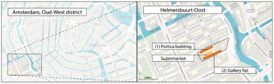
Figure 1.
Location of the case study in Amsterdam.

Table 1.
Identified components within the system boundaries that are considered suitable for the new energy system.
2.1.1. Greenhouse
In scenario 2, a rooftop greenhouse is added to this city block and plugged into the local energy system. Since this study is exploratory in the field of urban energy management, certain factors that would be constraining in practice are not considered or assumed positive. This means building regulations or municipal zoning plans are ignored, investment or maintenance costs are not considered and the existing substructure is assumed suitable to support the urban farms. In this city block, the rooftop greenhouse can only be placed on top of the residential buildings since the ground-level supermarket building, located in the courtyard, would be shaded most of the time. This lack of sunlight is confirmed by the solar atlas tool by the Amsterdam municipality [20].
In respect to the energy system, the key purpose of the added rooftop greenhouse is to act as a solar collector in summer and collect sufficient thermal energy to (1), heat itself during the winter months and (2), to provide a high-temperature energy source for the heat pump of the dwellings. The dimensions of the greenhouse footprint are constrained by the outer dimensions of the residential substructures, as such the maximum possible greenhouse floor area can be 78.8 m × 10.8 m (851 m2 in total) on top of the tenement building (1, Figure 1) or 107 m × 7.8 m (835 m2) on top of the gallery building (2, Figure 1). An overview of the shape and main structural dimensions and facade properties of the greenhouse can be found in Appendix A.2. The greenhouse is imagined as an archetypical glass structure on a concrete floor and the rooftop is designed under an inclination to allow for water runoff. The greenhouse is modelled as a single rectangular crop production volume, hence any crop processing and packaging stations, storage rooms or other supportive spaces are not taken into account.
2.1.2. Supermarket Building
The discussed supermarket (exploited by Lidl Nederland, Huizen, The Netherlands) is located at the ground level of this city block, partly enveloped by the surrounding dwellings. Only the sales floor, by far the largest space inside the supermarket building, is taken into account for the calculation of the energy profile. The interior dimensions of this space measure 15.4 m × 46.0 m × 2.9 m . The electricity consumption of this supermarket was 256 MWh in 2015 and 258 MWh in 2016; for the calculations in this study we apply the average of the two (personal communication, 2017).
2.1.3. Dwelling
Two buildings are located within the demarcated system boundaries that are considered suitable to be included in the local energy network. The first building is a 1926 tenement complex (1), composed of a concatenation of 6 clusters made up of 8 dwellings. One dwelling is missing to make space for a passage to the inner courtyard, leaving 47 households in total. The second building is a gallery building completed in 1965, with a total number of 68 apartments (2). Both buildings provide a large, rectangular shaped and flat rooftop surface (assumed) suitable for a rooftop glass structure and both buildings have been designed with a certain degree of constructive and architectural repetition, making any structural interventions more likely.
2.2. Performance Indicator
All three scenarios are assessed on their carbon equivalent emissions (CO2e) consequential to the demand for final electrical and thermal energy resources, see Table 2. In scenario 2, the heating and cooling systems of the dwelling, supermarket and greenhouse are synthesized and electrified, which puts additional demands on the national electricity grid. The underlying aim in the design of scenario 2 is to satisfy energy demands with onsite renewable energy production. This study focuses on solar thermal energy as an alternative to gas or district heating, consequently meaning that electricity must still be imported from across the system borders, for which standard grid mix electricity is used.
Table 2.
Inventory of greenhouse gas emissions of relevance to this study.
This paper evaluates the environmental impact of the built environment by assessing the footprint of CO2e, corresponding to the three main greenhouse gasses released into the atmosphere, multiplied by their 100-year global warming potential (GWP), i.e., carbon dioxide (CO2, GWP = 1), methane (CH4, GWP = 28) and nitrous oxide (N2O, GWP = 265). The GWP indicates the potential greenhouse effect of an emitted gas relative to an equivalent mass of carbon dioxide, measured over a period of 100 years after its release into the atmosphere [24].
2.3. Energy Balances
Steady-state thermal energy balance equations are solved for the greenhouse and the supermarket for every hour during a period of one year, resulting in 8760 energy fluxes (Heating/Cooling, H/C) that are aggregated into an energy profile for further evaluation and design (Section 2.4). The measured energy demand of the dwelling is converted into an hourly demand to align with the other components; see Section 2.3.2. This hourly approach allows us to generate a detailed representation of the components’ energy profiles, as for every hour the external climatological factors can be applied. In addition, heat loads that are periodical can be accurately (de)activated according to their time schedules, and diurnal patterns of heating or cooling demand can be precisely calculated instead of relying on assumptions or correction factors. Hourly measurements of the ambient air temperature (), solar heat load (), wind velocity () and relative humidity () are based on NEN5060 climate reference data [25]. An extensive Microsoft Excel worksheet is employed to calculate energy balances, to generate energy profiles for the three buildings and to adapt various parameters in order to establish a thermal energy equilibrium within the system as a whole.
2.3.1. Energy Balances: Supermarket
Many supermarket buildings in The Netherlands have a continuous heat surplus due to the cooling loads coming from both product display coolers, as well as sales-floor cooling. Recently built supermarkets come with an integrated system, where the back side heat from the displays is directly removed from the sales floor and exhausted into the atmosphere, occasionally reusing (a part of) it for heating purposes. The supermarket in this study does not have this modern system and works with individually operating cooling units, where excess heat is exhausted into the space. Nowadays, supermarkets are expected to install glass doors to cover the cooled product displays in order to contain the cold. A direct consequence of this is the necessity to mechanically cool the sales floor to prevent unwanted condensation on the cold surface of the glass doors. Energy balance equation 1 is used to calculate the cooling demand of the supermarket. The equation only describes the thermal balance of the sales floor and does not take into account the rejected energy generated by the product cooling units. For the calculations in Section 2.5 this study is assuming that the exhaust air coming from the climate control system pivots around 35 °C throughout the whole year.
The various components of the supermarket energy balance equation and the applied parameters are further specified and explained in Nomenclature section and Appendix A.1.
2.3.2. Energy Demand: Dwellings
The thermal energy demand from the tenement building (building 1) and the gallery flat (building 2) are not manually calculated with energy balance equations. Instead, they are retrieved from publicly available datasets provided by the regional network manager Liander [26]. Liander gathers and publishes the annual gas and electricity demand of all addresses connected to its network (in an anonymized form). Annual gas consumptions are converted into an hourly representation so they can be compared with the energy profiles of the supermarket and the greenhouse. For this we use the caloric value of Dutch natural gas of 35.17 MJ/m3 [22]. In addition to the total energy demand, Liander also published a predictive dataset of hourly fractions of the annual gas and electricity use, based on secondary data from +10.000 customers and normalized for the average temperature profile of the past 20 years, Figure 2 [27]. Gas used for cooking purposes is not addressed separately in this study as it represents a negligible amount (3.9%) relative to the total gas consumption [28].
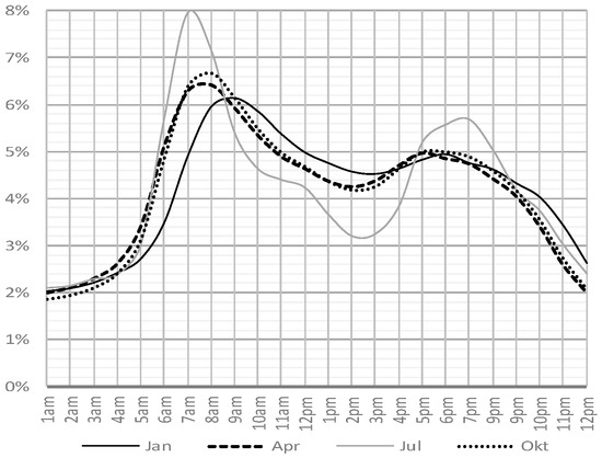
Figure 2.
For exemplary purposes: 24 h gas demand curve for an average household in NL, based on Liander data. The % represents the demand for that hour relative to the daily total. Two peaks are evident for each of the four curves: a morning peak when people wake up, turn on the heating and have a shower and an afternoon peak, when people tend to cook dinner (on gas stoves) and switch on the heating (again).
In both scenario 2 and 3, all the apartments are assumed to have undergone an impactful energy renovation, increasing the energy performance up to energy label B. Based on the research conducted by Majcen [28] on the actual gas consumptions vs. theoretical gas consumptions of dwellings relative to their ascribed energy labels, the reductions in gas demand due to the renovation can be estimated. The gas demand of the gallery building should be diminished with 7% (from energy label C > B) and the demand of the tenement building drops with 26% (D > B or E > B, average is 26%), see Table 3. It is expected that the theoretical renovation provides sufficient additional thermal insulation that a comfortable indoor temperature can be maintained by medium-temperature heating systems operating at 45 °C.
Table 3.
Current demand for energy resources by the residential buildings (hh = household) and estimated gas demand reduction after renovation.
It is relevant to understand how the energy demand for space heating (SH) and energy demand for domestic hot water (DHW) relate to each other due to their different temperature requirements. For the DHW, a set point temperature of 55 °C is used as a calculation value. In practice, the heat pump will boost the temperature of the water periodically up to a minimum of 65 °C to prevent legionella from developing in the system, but this peak is neglected for the energy calculations in this study. Schepers et al. estimate that in a well-insulated 1900–1945’s dwelling, the gas demand for DHW would be 40% of the total gas use on an annual basis [29]. In practice there would be zero to limited gas demand for space heating during the summer months. However, this ratio is still projected to every hour of the year, due to the unavailability of correct consumption data at the hourly level.
2.3.3. Energy Balance: Greenhouse
The rooftop greenhouse is the new component added to the existing built environment and acts as a solar collector, capturing thermal energy from the sun through floor cooling. The interior temperature ( of this greenhouse is governed by the exterior climate, the energy transfer across the building skin and the resulting interior energy fluxes. Tin at time (t) can be calculated with Equation (2) and builds upon the temperature calculated at (t − 1) by assuming the heat flows are stationary during the time-step from t − 1 to t ( and includes the effect of thermal inertia. In this calculation time steps (t) of one hour are used.
represents the energy deficit (H, positive flux) or excess (C, negative flux) relative to the intended minimum of maximum greenhouse indoor temperature and and is further specified in Equation (5a,b). The total thermal capacity is the sum of the thermal effective components in the space and is calculated with Equation (3):
For simplification purposes, only the greenhouse air ( and the thermally active layer of the concrete greenhouse floor with mass mn (kg) and specific heat capacity cn (J/kg·K) are included in the calculation. The top 80 mm concrete corresponds approximately to and is based on the energy demand by the thickness of the concrete layer active in the diurnal thermal exchange cycle.
The energy balance of the archetypical greenhouse with solar energy as its main source for photosynthetically active radiation contains several passive and active fluxes, as defined in Equation (4), adapted from Sabeh [30]. The greenhouse is assumed to be a closed system, hence ventilation related energy fluxes are excluded.
The dominant fluxes across the façade are the result of solar radiation and ambient temperature and are respectively noted as (W) and (W) for conductive, convective and radiative transmission. These fluxes influence the greenhouse climate and consequently the dominant interior exchange: the latent () and sensible () heat exchanged by crop transpiration, (W). (W) represents the heat transfer by infiltration and is related to the outdoor wind speed. Greenhouse thermal emissivity to the external hemisphere is noted by (W). The total interior heat gain is described by (W) and consist of , and , respectively thermal heat gain by active equipment, installed artificial lights and present workers/visitors. is determined by the set points for minimum greenhouse indoor air temperature during photoperiod (, minimum indoor air temperature during dark period ( and maximum indoor temperature (°C). When the (combined) heat influxes produce high indoor greenhouse temperatures, the redundant thermal energy is removed by means of floor cooling, (W). When the thermal fluxes to the external environment exceed the combined influxes and the minimum indoor set point temperature is passed, thermal energy is added to the greenhouse by means of floor heating, (W). Equation (5a,b) isolate or and builts upon the indoor temperature calculated at (t − 1). The positive thermal flux , i.e., heating, activates if or at (t − 1) and , i.e., cooling, is active when at (t − 1). Equation (5a,b):
The various interior and exterior fluxes of the energy balance, used equations, applied parameters, structural properties and other factors are described in Appendix A.2. The last section of Appendix A.2. discusses the effect of the food crops on the energy balance of the greenhouse.
2.4. Energy Profiles
The outcomes of the energy balance equations (Equations (1) and (5a,b)) and the dwelling thermal energy demand are aggregated into a matrix of 24 h by 365 days (Figure 3a–c), in this study coined energy profiles, and are used to locate and quantify the simultaneous and mismatched discrepancies between thermal energy excesses and demands. In the visualizations below, orange indicates an excess of thermal energy, i.e., a cooling demand in order to maintain the intended temperature set-point . Blue represents a heating demand, i.e., a deficit of thermal energy relative to the intended minimum indoor temperature. The intensity of the color depicts the height of the heating/cooling demand. The 3D Figures represent monthly totals (kWh) and emphasize the seasonal, daily demand patterns and weather influences and show how the energy profiles relate to each other in terms of magnitude.
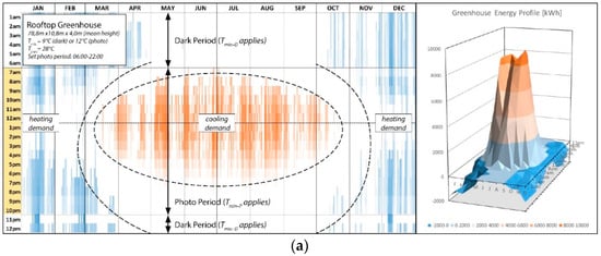
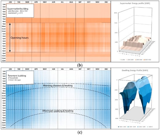
Figure 3.
(a) Greenhouse: the energy profile of the greenhouse shows a white transition zone when the greenhouse indoor temperature is within the desired range. Temperature set points and photoperiod used for the initial situation are mentioned in the figure. (b) Supermarket energy balance: The supermarket has a year-round cooling demand, ranging from 2 kW in winter up to 40 kW during peaks in summer. The building does not have a heating demand at any moment of the year. (c) Dwellings: the hourly demand for thermal energy is ranging from 4 kW for some warm hours during nights in August, up to peak heating demand of 147 kW during January mornings. The dwellings are not actively cooled, as is common practice for this architectural typology in The Netherlands.
2.5. System Integration
To overcome the seasonal mismatches between supply and demand, an aquifer thermal energy storage (ATES) is proposed (Section 2.5.1). The new energy system is introduced and discussed in Section 2.5.2 and is reversible, providing both a summer setting (Section 2.5.3) and winter setting (Section 2.5.4) to serve the core purpose of both heating and cooling. The design of the integrated energy system is not supported by calculations at the level of the individual system or utility (i.e., flow rate) but remains abstract as more detail would not contribute to the intended aim of this study.
2.5.1. Aquifer Thermal Energy Storage
Excess thermal energy that is extracted from the greenhouse volume by means of floor cooling (medium = water) needs to be buffered over the season. Considering that the local energy system operates on low temperatures, serves a city block and surface space is limited in this inner-urban context, an underground doublet aquifer thermal energy storage (ATES) is considered the most suitable method to tackle the seasonal mismatch between heat excess and heat deficits. Underground energy storage is characterized by both high storage efficiencies and capacities. Open-loop ATES systems store sensible heat in water-rich earth layers (the aquifers), using the groundwater as the transport and storage medium, subtracting and injecting warm and cold water between the respective wells [31]. Low-temperature (T < 25 °C) ATES systems are prevailing (99%) over high-temperature systems and about 85% of all systems is located in The Netherlands, where the soil offers favorable hydrogeological conditions and where the climate has substantial seasonal variations in ambient temperature to make an ATES effective [32].
One way to express the thermal performance of an ATES is by looking at the thermal recovery efficiency (), the fraction between the energy injected and retrieved. The energy recovered from a well is generally lower than the energy injected due to dissipation losses to the surroundings and advection due to local groundwater flows. Calculating the exact recovery is complicated, as many site-specific hydrological parameters are involved. It also depends on system-specific factors such as the injection temperature, the deviating pumping volumes between seasons because of demand patterns and the distance between the warm and cold well. Sommer et al. mention a numerically modelled recovery value of 75% in a stagnant aquifer [33] (no groundwater flow) and report a 65% storage recovery from the warm well and a 82% cold recovery based on field measurements [34]. Another report by Steekelenburg et al. [35] mentions a higher efficiency between 85–90% over a period of 180 days. Considering the uncertainties and small scale of these particular systems, this study applies a conservative ATES efficiency () of 0.75 for both the warm well and the cold well.
To avoid systematic heating or cooling of the subsurface over time, which would disturb the ground water quality and eventually lead to ineffective and unsustainable system performances, Dutch provincial regulators require a thermally balanced system [36]. Most provinces in The Netherlands include a clausal in their groundwater act permit prescribing an energetically balanced system. Due to unpredictable climatological circumstances, certain deviations in the ATES balance are allowed. One province (Noord-Brabant) allows a 15% deviation from this balance for a 5-year period and a 10% deviation over a period of 10 years [37], but also balance requirements within 5 years are reported [38]. A field study on the balances of Dutch ATES systems revealed that the average energy balance for utility projects is +5% (n = 56) i.e., less heat is extracted than cold, and for residential ATES systems −34% (n = 5), meaning less cold gets extracted than heat [39]. Energetically balanced urban functions (combining both heat- and cold-demanding functions in a certain urban area) therefore are paramount. To correct for storage unbalances, regenerative mechanical ATES cooling or heating could be employed, but this option is not considered for this study. For COP calculations (Section 2.5.3), the average water temperature in the warm well is assumed to drop with 3 °C between seasons and the cold well water temperature remains unaffected.
2.5.2. System Configuration
The local energy system inter-connects four components: the dwellings, the rooftop greenhouse, the supermarket and the ATES. The system is reversible, providing a summer and winter setting to serve the core purpose of both heating and cooling. The greenhouse is the only component that shows both a heating and a cooling demand and is therefore decisive in determining the cooling and heating period for the entire system. Figure 4 shows the indoor temperature of the greenhouse without any mechanical heating or cooling and without energy exchange with the supermarket. The diagram is based on greenhouse configuration temperatures: . The configuration of the whole energy system, i.e., the period when thermal energy is stored and when it is extracted, is based on the indoor greenhouse temperature, which correlates with thermal energy excess or deficit. The months April and October evidently show a mixed demand for heating (morning + evening) and cooling (afternoon). Considering that greenhouse cooling can be achieved passively by opening up windows at the expense of losing thermal energy to the ambient environment, these two months are set to heating mode. This means that the cooling period is set to May–October (6 months); the other half of the year the system is set to heating mode. For simplification, a full month round-off applies and no in-between system reverses are included.
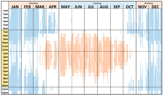
Figure 4.
Indoor Greenhouse temperature (°C). Initial set point temperatures: Tmax = 28 °C, Tmin-D = 9 °C, Tmin-P = 12 °C. Blue indicates that Tmin has been reached or supassed, red indicates that Tmax has been reached or surpassed and white indicates that the GH indoor temperature is within desirable range. The yellow hatched hours indicate the photoperiod (PP) timeslot.
Figure 5 gives an abstract representation of the energy flows within the new local energy system and the medium temperatures where relevant. In the following sections first discusses the winter configuration (point 1–5, left), followed by the summer configuration (point 6–8, right).
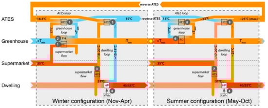
Figure 5.
Abstract representation of the thermal energy flows in scenario 2a–d: the local system. Relevant medium/component temperatures are mentioned where~indicates an estimated temperature. FH = floor heating, FC = floor cooling, HE = heat exchanger. The ATES reverses at the beginning of May, when the cooling season starts and at the end of October, when the heating season starts. The temperature of the warm well of the ATES is assumed to drop with 3 °C between seasons (see Section 2.5.3).
2.5.3. System Configuration: Winter
The local energy system operates for two core purposes: heating in winter and cooling in summer, as shown by Figure 5 and Figure 6. During winter, the supermarket exchanges thermal energy through a heat exchanger (medium = air) with the greenhouse when , point 1 in Figure 5. When the greenhouse is within the accepted range, the energy system uses the excess thermal energy from the supermarket to increase the temperature of the warm water () coming from the ATES warm well. The water is boosted from ±18.3 °C (estimated ATES water temperature) to 31 °C, with the aim of increasing the COP of the heat pump, thereby reducing the electrical energy investment (point 3 & 4). The efficiency of the air-to-water heat exchanger is assumed to be 90%. If the supermarket cannot provide sufficient energy to maintain a suitable greenhouse indoor temperature, warm water from the ATES is pumped through the floor of the greenhouse (point 2), which simultaneously drops the temperature in the loop and charges the cold source of the ATES. Here, an exchange efficiency (water-water) of 90% is applied (point 5). The heat pump output flow is used to charge the ATES cold source; again an exchange efficiency of 90% applies (point 5).
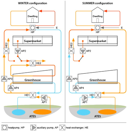
Figure 6.
Position of the Auxiliary pumps (AP), Heat exhangers (HE) and Heat Pumps (HP) within the local energy system for both system configurations.
Equation (6) calculates the minimum amount of thermal energy that should be stored in the ATES annually () and is based on the energy demand by the greenhouse ( and the energy required by the dwelling (), taking into account the efficiency (η2 = 0.9) of the heat exchange (HE2, Figure 6) between the ATES loop and the GH & DW loop and the ATES recovery efficiency ().
The stored thermal energy reserved for the greenhouse, (W) can be calculated with Equation (7). If the greenhouse’s interior temperature , surplus energy () from the supermarket in the form of warm air () is shared with the greenhouse, taking into account the efficiency of the heat exchanger (HE2, η = 0.9). When this energy flux is insufficient to maintain a suitable indoor greenhouse temperature, additional energy is retrieved from the ATES.
Equation (8) is used to calculate the stored thermal energy reserved for the dwelling, (W). Since the thermal energy provision of the dwelling involves a heat pump, electrical energy E is converted into thermal energy and becomes part of the total energy required, . When , the energy rejected from the supermarket () is used to pre-heat the heat pump approach water () from ±18.3 °C (estimated ATES extraction temperature, see Table 4) to approximately 31 °C, based on a heat exchange efficiency of 0.9 (HE3). The Coefficient of Performance of the heat pump (COPHP) is estimated from the Carnot efficiency, with an assumed practice efficiency () and varies throughout the year due to the two possible approach temperatures (18 °C if straight from the ATES or 31 °C if upgraded) and two different upper temperatures: for SH and for DHW.
where is the electrical energy demand from the heat pump at moment (t):
where the COP is calculated with Equation (10):
Table 4.
Different values applied for Tlow and in the calculation of the heat pump COP (Equation (10)). DHW & SH constitute respectively 40% and 60% of the total energy demand (Section 2.3.2).
(°C) is the approach temperature of the water passing through the heat pump. When the energy rejected by the supermarket is not used to heat the greenhouse, it will be used to increase the COP of the heat pump. represents the efficiency of the heat exchange between the supermarket warm air and the heat pump approach water (HE3) and is set to 0.9. The temperature of the supermarket exhaust air is noted by (°C) and is assumed to be around 35 °C. An overview and explanation of the various values for and can be found in Table 4. represents the ratio of the real COP in practice to the Carnot COP; it is set to 0.5 [40].
2.5.4. System Configuration: Summer
In summer, the system functions similarly to the winter configuration. Cold water ( that was previously stored in winter, is now discharged with the sole purpose of cooling the greenhouse by means of floor cooling (point 6). During the process, the cooling water warms up to approximately , after which it can recharge the thermal well of the ATES (point 8). In summer, the full capacity of the supermarket excess energy is used to preheat the tap water and the water in the heat pump loop, again narrowing the temperature jump and increasing the COP (point 7). The outflow of the heat pump (point 4) is used to charge the ATES heat source (point 8) and this temperature is assumed to be around 25 °C. The total cooling energy (that should be stored by the ATES is calculated by Equation (11). As mentioned, only the greenhouse is supplied with cooling energy from the cold well. (kWh) is the cooling demand greenhouse at (t).
In summer, the excess energy from the supermarket is used in its full capacity to narrow the temperature increase within the heat pumps of the dwellings, similar to the winter setting. The warm air is passed by the return loop of the heat pump, preheating the water up to a temperature of around 31 °C. The COPHP and the required electrical energy are calculated with respectively Equations (9) and (10).
2.5.5. System Configuration: Additional Electricity Demand
The local energy system consists of four sub-flows that are put into motion by electrical pumps: (1) the ATES loop, (2) the greenhouse loop, (3) the dwelling loop and (4) the supermarket air flow (Figure 6). The added emissions due to the electricity consumption of these pumps is included in the carbon evaluation of the system. The ATES doublet loop pumps water between the warm and the cold well (or vice-versa) whilst extracting the cooling or heating energy with a water-to-water heat exchanger (HE1). The warm air from the supermarket cooling system is either pumped towards the greenhouse or the heat pump of the dwellings, where thermal energy is exchanged with the dwelling flow. The dwelling flow circulates between the heat pump of the dwellings and the heat exchanger of the ATES flow, where the flow is preheated by heat exchange (HE3). Finally, there is the greenhouse flow, connecting the greenhouse floor heating/cooling system with the ATES flow. As this study does not get into systems level detail, the power of the electrical pumps remains an estimation.
The greenhouse lighting system switches on when the photoactive radiation (PAR) from the sun drops below 30.6 W/m2 (corresponding with 140 µmol/m2/s PPFD, see Appendix A.2) and when time (t) is within the scheduled photo period. To account for operational activities within the greenhouse that do not relate to cooling, heating or crop lighting, a value of 5 kWh/m2/year is assumed [41]. An overview of the aforementioned electrical demands related to the auxiliary pumps (AP) or the greenhouse can be found in Table 5.
Table 5.
Electrification of the system. Overview of auxiliary pumps, greenhouse crop lighting and operational activities.
2.6. System Configuration: Balance
For a durable performance of the ATES, the stored/retrieved thermal energy should be in balance with the stored/retrieved cooling energy. The fraction in equation 12 is used to determine the balance of the ATES for one summer-winter cycle. An outcome above 1.00 indicates that the heating demand is exceeding the capacity of the warm well. This could, for example, imply that insufficient thermal energy is extracted from the greenhouse during summer or that the heating demand is too high. An outcome below 1.00 reveals that more thermal energy is stored in summer than is used during winter. In The Netherlands, an ATES balance may be achieved over multiple seasons as predicted estimated demands and actual energy demands do not always overlap. This study aims for an annually balanced ATES, still, minor deviations from 1.00 are considered acceptable. The system can be brought into balance with hard and soft reconfigurations. Hard reconfiguration are physical modifications of the system, for example (dis)connecting a certain number of household to lower the heating demand or increasing the size of the greenhouses. The greenhouse functions as the main control component of the system. Soft configurations imply changes in the greenhouse indoor environment that directly affect its energy balance and therefore the system-performance. For example, lowering the cooling set point to increase the extracted solar energy. In this study, system balancing is a process of trial and error with earlier mentioned calculation model.
Figure 7 (left) points out the unbalance if both the tenement building (47 hh) as well as the gallery building (68 hh) were to be supplied by one single rooftop greenhouse. Applied indoor climate and other relevant configuration specifications are listed per scenario in Section 3.4. The combined demand for heating by the dwellings plus the greenhouse exceeds the thermal energy that can be extracted from the greenhouse over the summer. Even when the is dropped to 25 °C, insufficient energy can be extracted from the greenhouse to heat the dwellings. Figure 7 (middle) corresponds with scenario 2a and shows that a balance can be achieved when only the tenement building is connected and if is set to 26.0 °C. The right graph in Figure 7 shows the ATES balance if the greenhouse solar collector would be placed on top of the gallery building and is set to 27 °C. The carbon evaluation in the results chapter continues with the tenement building + greenhouse + supermarket combination, but could be repeated similarly for the configuration with the gallery flat.
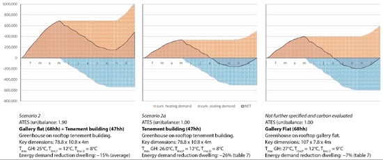
Figure 7.
(Dis)charging of the ATES. Both the tenement building as the gallery building can be heated by means of a rooftop solar collector, provided that the system is configured under specific climate settings. Scenario 2 & 2a correspond with the scenarios described in Section 3.4.
3. Results
Carbon accounting of all used energy resources is used to determine the CO2e footprint of the three scenarios of this case study.
3.1. Scenario 1: Carbon Footprint Business as Usual (BAU)
The apartments in the tenement building (n = 47) use on average 1114 m3 of natural gas per year for space heating, cooking and domestic hot water. For the carbon calculations in the BAU scenario it is assumed that none of the apartments is making use of electric cooking or heating systems. The average annual electricity consumption of the apartments is 1805 kWh/year. The supermarket is all-electric and consumes 257 MWh of electricity per annum. The electricity demand by the residential building and the supermarket combined with the use of natural gas leads to a total carbon emission of 274 tons annually, see Figure 8.
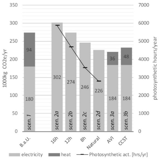
Figure 8.
Scenario analysis: BAU, local energy system (scen. 2a–d), district heating method (3a,b). AVI = waste incineration based district heating system, CCST = power plant waste heat based district heating system.
3.2. Scenario 2: Environmental Footprint Greenhouse Solar Collector
In the balanced local energy system, the gas use of the tenement building is fully substituted with renewable solar thermal energy, which is extracted from a greenhouse that fits on the rooftop of the same building (851 m2). This leads to a carbon cutback of 94 ton/year. The greenhouse and the system introduce an additional electricity demand to the national grid. The change to heat pumps and electric cooking adds 51 MWhE/year and 8 MWhE/year annually. Auxiliary energy required for the internal system pumps add an estimated 20 MWhE. The electricity demand from the dwellings and the supermarket, 84 & 257 MWhE, remain unaffected by the new energy system. The greenhouse-related electricity demand is composed of 4 MWhE for operational activities and 149 MWhE for crop growing lights when the optimal crop growing conditions regarding the greenhouse’s indoor temperature and PPFD are maintained (scenario 2a). The carbon emission corresponding with all aforementioned energy demands cumulates to 302 ton/year, which is a 28 ton increase compared to the initial BAU scenario, see Table 6. The carbon performance of scenario 2 is primarily controlled by the set photoperiod (PP). Would this be shortened to 12 h, 8 h or be fully deactivated, the annual cumulative carbon footprint of the full system drops to respectively 268 (−6 ton relative to BAU), 246 (−28 ton) or 226 ton (−53 ton).
Table 6.
Carbon accounting: inventory of consumed resources and corresponding carbon footprints. Scenario 2a and 2d correspond with scenario 2a and 2d described in Section 3.4 and are in ATES balance.
3.3. Scenario 3: Environmental Footprint Amsterdam District Heating
In scenario 3, the residential building is connected to the existing Amsterdam heat grid. Currently, there are two individually operating heat grids in the city, which are heated by two different sources. The North-West network is fueled by the Amsterdam waste incineration plant (Amsterdam Energie Bedrijf, or AVI) and a biodiesel factory and is exploited by Westpoort Warmte. The South-East network is energized by a Combined Cycles Gas Turbine (CCGT, Dutch: STEG) power station and is exploited by NUON-Vattenval [42]. At the moment these two networks primarily serve the inner urban ring, but future plans include a coupling between the two systems and a grid expansion towards both the region, as well as the inner-city. Current plans intend to make the district heating system fully renewable by 2040. This goal in itself seems feasible, but due to uncertainties surrounding the development of required technologies, exact potential, timeline and costs, the specific mix of various renewable sources cannot be predicted and remains speculative [43]. This study therefore performs the carbon assessment based on the present methods.
The case study location is in close proximity of branches from both heat grids [44]. To the extent of the authors’ knowledge there are no urban plans available to accurately determine which parts of the city will be connected to which network in the future. Therefore, this study considers both networks as a possible option and includes both for carbon evaluation. The district heating systems deliver high temperature water of around 70–90 °C at the end-user, which is considered sufficient for both SH and DHW. Hence, this study assumes no additional heat pumps are necessary and a heat exchanger will suffice.
In 2016, CE Delft published updated carbon footprint values for centralized heat generation technologies, which also include the two aforementioned methods. The footprints are based on conservative calculations, consist of direct and indirect carbon emissions released during the generation of heat, take into account generally accepted average transportation losses (15%) and include a coefficient to account for the reduction in electricity generation due to the removal of steam for heat generation. For a detailed description of the calculation methods applied and aspects included, see the report by CE Delft [23]. Should the tenement building be connected to the heat grid connected to the waste incineration plant, the cumulative CO2e footprint would become 220 ton/year (Table 6 and Figure 8), based on a carbon footprint of 26.5 kg CO2e/GJ (listed in Table 2). If a connection is made with a branch of the CCGT heat grid, the annual emission of the buildings becomes 232 ton, based on 36.0 kg CO2e/GJ. Similarly to scenario 2, this scenario also assumes that the dwellings are energetically renovated.
3.4. Configuration: Optimal Growing Climate or Optimal Energy Performance
In the calculation model, the minimal indoor temperature of the greenhouse is coupled with the photo activity of the crops, which is in this study only determined by simultaneous suitable key conditions for indoor temperature and PPFD, respectively and PPFD = 140 µmol/m2/s. A desired PPFD can be reached naturally by letting in solar radiation or can be managed by supplementary artificial crop lighting for the duration of the specified photoperiod (PP). This study does not model agricultural productivity separately, but by counting the hours in which both key parameters show the desirable growing conditions, preliminary statements on the greenhouse productivity can be made. If the PP is shortened with the purpose of reducing the carbon footprint of the lighting system, concessions on the greenhouse productive hours have to be made. A photoperiod of 16 h (06:00–22:00) is considered optimal and corresponds with 5893 photosynthetic active hours per year. Narrowing this PP window to 12 h (06:00–18:00, scen. 2b), 8 h (08:00–16:00, scen. 2c) or completely deactivating supplementary growing lights (scen. 2d) diminishes the photosynthetic active hours to respectively 4456 (−4%), 3534 (−40%) and 2775 h (−53%). The growing lights produce a significant internal thermal gain and modelling points out that the heating demand of the greenhouse increases when the PP is shortened. To compensate for this, the heating set point temperature in scenario 2c and 2d has to be increased in order to maintain system equilibrium. An overview of the key system parameters used to achieve system-equilibrium for various tested scenarios can be found in Table 7 below.
Table 7.
Various system configurations. Overview of relevant parameters and their values. Scenario 2a–d are all in balance, but differ in photoperiod duration. Key greenhouse dimensions: 10.8 m × 78.8 m × 4 m (mean), orientation: 66° relative to North (building 1 in Figure 1).
4. Discussion
4.1. Sensitivity Analysis (SA) Assumed Parameters
For reasons of simplification or due to lack of applicable data from literature, certain parameters represent assumed values. Four of these are tested in a sensitivity analysis: ,, and the power of the ATES pump, . The efficiency parameters (η) are tested with incremental steps of ±5% (Figure 9 right). is tested with incremental steps of ±10% (Figure 9 left). The parameters and are assessed based on their impact on the total carbon emission of the system (ton/year). The parameters and primarily influence the energy losses within the system and are therefore assessed on the total thermal energy that should be extracted from the greenhouse in order to carry the system over the following winter. In other words: a decrease in efficiency leads to an increase in heat extracted in order to compensate.
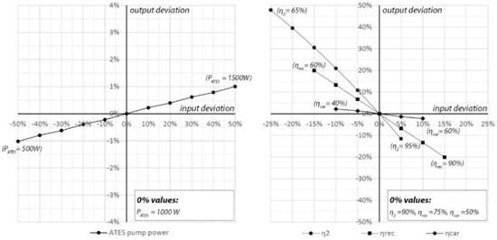
Figure 9.
Sensitivity analysis of four parameters. Left: . Right: , and .
Efficiency accounts for the energy losses during the energy exchange between the greenhouse floor cooling/heating circuit and the ATES and is set to 90%, an acceptable value for modern heat exchangers. The SA indicates a strong correlation between the overall storage efficiency of the system and the value used. Hard system reconfigurations might be required to reestablish a balanced system should become too low, for example disconnecting some households.
An ATES recovery efficiency () cannot be captured in a generic representative value as it is depending on too many physical, geological and system characteristics. Performances found in practice represent a range of efficiencies, for that, is set to a conservative 75%. An increase from 75% to 90% would reduce the minimum required extracted thermal energy with 20%, or expressed in terms of system scale: 20% more dwellings could be added to the system.
In practice, Carnot efficiencies of heat pumps range between 40% and 60%, hence the in this study is positioned in the middle: 50%. Applying a 40% or 60% Carnot efficiency results in a ±~2% deviation in the output, i.e., a slight in or decrease of carbon emissions.
Estimations are used to describe the power input for the auxiliary pumps. The SA is limited to the ATES pump only as it is the most powerful pump that is considered and it is in operation year-round, making its analysis representative for the other auxiliary pumps that are less powerful and/or show fewer hours in operation. Deviating 50% from the assumed leads to a marginal ~1% carbon emission increase.
4.2. Research Relevance
4.2.1. Societal Relevance
Urban rooftop solar collectors can provide parallel benefits to the generation of renewable thermal energy. The method is suitable for an architectonical and urban typology typically associated with (social) housing for middle or lower income classes; e.g., large gallery buildings, tenement buildings and older terraced housing rows. In The Netherlands, these buildings have been built in sixties and seventies in large numbers at the perimeters of towns and often form entire neighborhoods, providing a quick solution to a pressing housing need. Studies show a correlation between income levels and people’s food intake, showing unhealthy diets for the economically disadvantaged [45]. Visibly producing and retailing food crops in the locality could offer affordable and healthy alternatives to this social group, benefitting their physical wellbeing over a longer period of time. Coupling the horticultural activities with social programs for people with a distance to the labor market, introducing shared responsibility or working with co-ownership models could potentially lead to improved social cohesion within these neighborhoods [46].
4.2.2. Scientific Relevance
The applied methods in this study allow for an accurate representation of the proportions within the carbon inventory of the local energy system and how carbon competes with district heating. This study offers a first insight on the capacity and impact of a rooftop greenhouse solar collector for a specific case study and can serve as a stepping stone towards urban upscaling, systematization and a more detailed assessment. Even though this study is limited to the appraisal of energy, it points towards a neighborhood-level integrative design and holistic evaluation of all relevant resources, adding to the research gap surrounding the food, energy and water nexus (FEW nexus) that is currently prevailing at the regional, national or global level, as discussed in [47,48,49,50,51]. It will be at the local scale where policies and strategies turn into physical interventions and where policy makers can combine public, private and civic interventions in order to counter climate change with a larger fist [52].
4.3. Outlook
4.3.1. Upscaling the System and Future Use
Exclusively based on an energy and/or carbon assessment, a rooftop-based greenhouse solar collector as described in this study might already be feasible for one single dwelling, which would logically not be sensible from a technical, agricultural or an economic perspective. Further research should attempt to connect energetic feasibility with economic and agricultural feasibility and technical possibility. Greenhouse upscaling or clustering increases the effectiveness and productivity of the system as will the investment or operational costs be reduced.
4.3.2. FEW Nexus Assessment: Avoided Food Miles
The CO2e assessment in this study is restricted to energy resources: natural gas, grid electricity and district heat. Extending the evaluation list with other resources commonly found in the urban metabolism, for example waste water treatment, (organic) waste management and food, will change the inter-scenario proportions of the carbon inventory [53]. A holistic FEW nexus evaluation of the emissions for all scenarios will further encourage integrative and symbiotic design, subsequently leading to a cumulative carbon footprint presumably in favor of the integrative greenhouse scenario. Conventional produce can be replaced with locally (and organically) produced crops, potentially diminishing embodied food miles. Conversion of bio-waste into bio fuels can substitute fossil energy carriers. These are individual methods or technologies that fit the concept of circular farming and can be aggregated into the design of a modern urban rooftop greenhouse. Further research should develop an integrative assessment methodology for urban farming to inform policy makers and come up with a systematic design approach to couple agricultural flows with the urban flows with the aim to establish a symbiotic relationship that produces the lowest possible carbon footprint.
4.3.3. Agricultural Productivity
A greenhouse solar collector plugged into the center of a community combines the production of two desirable resources: healthy local food crops and renewable thermal energy. However, in accordance with the aim of this study, harvesting thermal energy has priority above agricultural yield. Carbon evaluation of all three scenarios point out that only when artificial growing lights are not used, the greenhouse solar collector becomes carbon competitive with the centralized district heating. According to this study, merely relying on natural sunlight to provide the desired PPFD drops the annual photoactive hours by 53%, from 5891 to 2775 h. A monthly breakdown reveals that during December and January, two months with the lowest outside temperatures and with the shortest daylight periods, less than 5% of the natural annual photosynthetic activity will occur, while at the same time, almost 60% of the heating demand takes place. From an energy-prioritizing perspective, it would be more efficient to shut down the greenhouse during these two months and use the stored energy to heat additional dwellings instead. Further research on crop growing cycles, possible use of alternative (cold climate) crops and also crop carbon accounting as described before, should lead to a balanced use and climate configuration of the greenhouse regarding the combined optimization of agricultural productivity, as well as thermal energy yield.
5. Conclusions
The metropolitan area of Amsterdam intends to become (nearly) fossil energy free by the year 2050. One of the adopted core strategies towards this goal is to disconnect the built environment from the natural gas supply and connect it to the existing city-wide heating grid. This paper aimed to demonstrate the value of considering local energy potentials and synergistic design at the city block level by evaluating and comparing the carbon emissions of an alternative scenario: employing a greenhouse solar collector. Comprehensive calculations and modelling of a case study show that it is energetically possible to substitute the natural gas demand of one tenement building (47 households) with solar thermal energy extracted from the rooftop greenhouse. This greenhouse solar collector fits within the rooftop area (851 m2) of that same tenement building, is kept under specific interior climate set points to maintain a balanced system and is co-heated by excess energy from an adjacent supermarket.
Carbon accounting reveals that even after a disconnection from the gas supply is accomplished, the cumulative carbon footprint of the local solution exceeds the business as usual scenario with 28 tons/year. This is primarily due to emissions related with additional grid mix electricity demand consequential to applying crop lighting. Only when artificial lighting is deactivated entirely and crop photosynthetic activity is solely based on natural lighting, the greenhouse solar collector method becomes carbon-competitive with the Amsterdam district heating. Shortening the daily artificial photoperiod in order to lower the CO2 emissions diminishes the photosynthetic active hours for crop growth. Setting a desirable photoperiod of 16 h per day leads to 5893 h of suitable crop growing conditions per year. Opting out of artificial lighting completely results in 2775 h of suitable growing conditions, a considerable reduction of 53%. This study points out that an urban rooftop solar collectors could be a suitable renewable alternative to conventional gas use or district heating. However, a system configuration to optimize energetic performance and minimize carbon emissions can lead to a reduction in greenhouse agricultural productivity.
Author Contributions
N.t.C.: conceptualization, methodology, software, validation, formal analysis, investigation, resources, data curation, writing—original draft presentation, visualization, project administration. L.G.: Software, validation, resources, writing—original draft presentation. M.T.: methodology, validation, writing—review and editing, supervision. A.v.d.D.: conceptualisation, writing—review and editing, supervision, funding acquisition. All authors have read and agreed to the published version of the manuscript.
Funding
This research was funded by Belmont Forum/JPI Urban Europe (SUGI projects), grant number 11314551. The APC was funded by Delft University of Technology.
Acknowledgments
In February 2017, the construction and real estate department of the Lidl Holland (Marcel Ganzeboom and Arnold Baas) approached the Delft University of Technology to engage into a joint effort with the intention of developing a company-wide strategy towards a circular economy. The data related to the Lidl supermarket and the urban case study used in this paper comes forth from this research collaboration. This paper is part of the SUGI Moveable Nexus research project (EU Horizon 2020 project, N 730254). Moveable Nexus (M-Nex) will develop innovative and practical design solutions through stakeholder-engaged living labs in six different bioregions around the world to move current FEW-nexus research towards implementation.
Conflicts of Interest
The authors declare no conflict of interest. The funders had no role in the design of the study; in the collection, analyses, or interpretation of data; in the writing of the manuscript, or in the decision to publish the results.
Nomenclature
| Symbol | Unit | Description |
| ATES | - | Aquifer Thermal Energy Storage |
| BAU | - | Business as Usual |
| CO2e | - | Carbon dioxide equivalent |
| COP | - | Coefficient of Performance |
| DHW/SH | - | Domestic Hot Water/Space Heating |
| GH/DW/SM | - | Greenhouse/Dwelling/Supermarket |
| hh | - | household |
| PAR | - | Photo Active Radiation |
| PPFD | - | Photosynthetic Photon Flux Density |
| W/m2K4 | Hemispherical Stefan-Boltzmann constant: 5.67 × 10⁻⁸ | |
| Pa | Water vapour pressure | |
| - | Climate specific standard values. For a sea climate, a = 0.55 and b = 0.005 | |
| ρcon | kg/m3 | Density concrete: 2500 kg/m3 |
| ρair | kg/m3 | Density air: 1.21 kg/m3 |
| ηrec | - | Recovery efficiency ATES storage, set to 0.75 |
| ηcar | - | Heat pump Carnot efficiency, set to 0.5 |
| η1 | - | Heat exch. eff. SM flow > GH air (HE1, Figure 6), set to 0.9 |
| η2 | - | Heat exch. eff. ATES loop > GH loop and DW loop (HE2, Figure 6), set to 0.9 |
| η3 | - | Heat exch. eff. SM flow > DW loop (HE3, Figure 6), set to 0.9. |
| Wlights | W | Power crop growing lights (54 W/m2 in this study) |
| vwind | m/s | Wind velocity (NEN5060 data) |
| qinf | m3/m2/s | Air exchange with environment due to infiltration |
| Vair | m3 | Air volume |
| Vinf | m3/s | Air exchange volume due to infiltration (supermarket calculations) |
| Vvent | m3/s | Air exchange volume due to ventilation (supermarket calculations) |
| U(n) | W/m2·K | Rate of transfer of heat through structure n |
| Tmin-P | °C | Minimum greenhouse indoor temperature, photoperiod. |
| Tmin-D | °C | Minimum greenhouse indoor temperature, dark period |
| Tmax | °C | Maximum greenhouse temperature |
| Tlow | °C | Approach temperature heat pump |
| Tin | °C | Indoor temperature greenhouse |
| Thigh | °C | Upgrade temperature heat pump |
| Te | °C | Outside ambient air temperature (NEN5060 climate data) |
| Tair | °C | Assumed air temperature of waste energy flow supermarket, set to 35 °C |
| rPAR | - | Coefficient to filter out solar radiation in the PAR range |
| ro | - | Façade orientation reduction coefficient (see Table A1) |
| qtrans | W | Thermal energy flux due to temperature difference interior-exterior |
| qsun | W/m2 | Thermal heat gain by solar irradiation |
| qsky | W/m2 | Atmospheric long-wave irradiation |
| qper | W | Thermal heat load per person present |
| qlight | W/m2 | Thermal heat load by active lights, supermarket |
| QLIDL_C | kWhT | Cooling energy demand supermarket, i.e., energy provided |
| qinf | W | Energy flux due to air infiltration through façade construction |
| QGH_C_ATES | kWh | Cooling energy demand greenhouse (GH), supplied by the ATES |
| qeq | W/m2 | hermal heat load by active equipment |
| qem | W | Energy flux due to sky emissivity |
| np | - | Number of workers/customers present |
| M( ) | kg | Mass |
| Isun | W/m2 | Total incoming global horizontal irradiance (NEN5060 climate data) |
| gglass | - | Solar transmittance coefficient.: fraction of the solar radiation that passes the glass |
| f(n) | - | Active/Inactive coefficient for GH and SM internal heat loads, set to (1) or (0) |
| E | kWhe | Required electrical investment heat pump |
| cLED | % | Efficiency crop growing lights |
| ccon | J/(kg·K) | heat capacity concrete, this study applies 840 J/kg·K |
| cair | J/(kg·K) | heat capacity air, this study applies 1005 J/kg·K |
| A(n) | m2 | surface area, façade or floor (Aglass/Afloor) |
| ∑QGH_H_ATES | kWht/year | Thermal energy demand greenhouse (GH) supplied by the ATES |
| ∑QDW_H_ATES | kWht/year | Thermal energy demand dwelling (DW), supplied by the ATES |
| ∑QATES_H | kWht/year | Total thermal energy stored in the ATES |
| ∑QATES_C | kWhc/year | Total cooling energy stored in the ATES |
| - | Emissivity of greenhouse cover material. Set to 0.97 for single pane glazing | |
| °C | Sky temperature at (t) | |
| - | Relative Humidity at (t), retrieved from NEN5060 climate reference data | |
| Pa | Saturated water vapour pressure | |
| - | Sky view factor. Set to 0.5 for an unobstructed hemispherical dome |
Appendix A. Energy Balance Equations
Appendix A.1. Supermarket Energy Balance
Energy balance Equation (A1) is used to determine the cooling demand of the supermarket.
In a supermarket building, the internal heat gains and the thermal energy exchange with the outside environment due to ventilation and infiltration (i.e., door openings), are strongly correlating with the opening hours. Outside of opening hours, the front and back door remain closed and the infiltration rate is set to zero. Heat gained from staff and customers working and walking in the supermarket varies through the course of the day and will show the highest loads during shopping peak hours. Lights are only switched on when people are present in the building. It is assumed that bake-off activities occur periodically throughout the day. The ventilation system is assumed to be CO2 controlled and is therefore only active during opening hours, plus one additional hour after closing. Figure A1 shows the time slots used for the calculation of , and . For these calculations it is assumed that the supermarket is open 365 days a year, from 8 AM to 8 PM. Any holidays or deviant opening hours on Sundays are not taken into account. Finally, (W) describes the amount of excess energy that should be removed from the sales floor to maintain a steady indoor temperature. The supermarket does not have any transparent surfaces, thus heat gain by the sun can be neglected.
The internal heat gain () that is coming from staff and customers present in the supermarket, heat gain from lighting, from equipment and heat coming from the bake-off section is calculated with Equation (A2):
The internal heat gain by the customers and staff present on the sales floor is noted by (W). In this study, a heat load of 130 W/person is assumed [54]. The number of customers (np) during a day is roughly estimated per hour (range = 10–75 persons) and can be found in Figure A1. Heat emitted by the ceiling lights and operational activities is noted by and respectively and for this study, a heat load of 10 W/m2 and 15 W/m2 are applied, which is in accordance with the value Lidl adopts for their own energy calculations (personal communication, 2017). The bake-off section of the supermarket’s bakery produces a lot of heat when the ovens are turned on and a value of 6000 W (i.e., ±8.5 W/m2) is added to the equation when the ovens are active. The periodicity of the internal fluxes is controlled by , , and (active = 1, inactive = 0) and follows the timetable in Figure A1.

Figure A1.
Hourly timetable of time based thermal fluxes for the super-market building.
Figure A1.
Hourly timetable of time based thermal fluxes for the super-market building.

Due to constant main door openings and multiple daily truck unloading at the back of the store, the heat loss by infiltration () of a supermarket building is significant; calculated with Equation (A3):
The uncontrolled air exchange () between the indoor and the outdoor environment is in this study set to 0.443 m3/s. The density of the air () is set to 1.21 kg/m3 and the specific heat capacity () is set to 1005 J/kg·K. The indoor temperature () on the sales floor is maintained on 21 °C all year round, a temperature generally low enough to prevent undesirable condensation on the glass display covers. Additional infiltration due to cracks and holes in the facades and roof of the building are ignored. The ambient outside temperature is noted by (°C).
Energy removed from the supermarket space due to mechanized air exchange with the outdoor environment for the purpose of ventilation () is determined with Equation (A4):
denotes ventilation rate, for which a value of 0.170 m3/s is applied. Ventilation only occurs during specific hours, noted by .
Heat fluxes across the façades, roof and floor depend on the difference between the external air temperature and the indoor air temperature and is represented by (W); calculated with Equation (A5):
The heat transfer coefficients for the roof, walls and floor () are 0.17, 0.22 and 0.25 W/m2K respectively. represents the surface area of these facades (m2). is set to 15 °C when calculating the energy exchange across the floor of the supermarket.
Appendix A.2. Greenhouse Energy Balance
The energy balance of the greenhouse is contained in Equation (A6):
Equation (A6) is converted into Equation (A7) to isolate the or (see Section 2.3.3). Equation (A9) (infiltration losses) and Equation (A17) (transfer across façade) are integrated in Equation (A7):
(W) represents the heat transfer by solar radiation and is denoted by Equation (A8). The total heat gain by solar radiation is calculated individually for each transparent façade.
The global horizontal solar radiation is noted by (W/m2) and is retrieved from weather data (NEN5060). The material properties of the single glazing glass façade are standardized: the thermal transmittance (U-value) is set at 5.7 W/m2K [55] and the solar transmittance coefficient () is set at 0.65 [56]. The central axis of the greenhouse has an angle of 66° relative to the North. Instead of using comprehensive trigonometric formulas, reduction coefficients () are applied to compensate for the non-optimal façade orientations in relation to the heat gain by global horizontal irradiance. Table A1. shows the for all facades. Since the glass roof is slightly inclined towards the North-West, we assume a reduction coefficient of 0.9 instead of 1.0. Only wavelengths in the NIR & UV (Near Infra-Red & Ultra Violet) range are accounted for, since PAR light (Photosynthetic Active Radiation) is directly processed by the plants, which is noted by the factor (0.475), which is discussed later in this section.
Even though the greenhouse is intended to be a closed system, there are structural imperfections and frequent door openings that cause exchange of air between the interior and exterior that affect the thermal balance of the greenhouse. This is calculated with Equation (A9):
In standard greenhouses, air exchange with the environment (m3/m2GH/s) is assumed to increase linearly with the wind velocity vwind (m/s), with a coefficient i of 0.00008 [55]. Energy exchange due to infiltration depends on the difference between the indoor and outdoor ambient air temperature Te (°C).
The combined internal heat load is described by (W/m2) (Equation (A10)) and consists of , and .
Heat gain coming from active mechanical equipment and operational activites is noted by a standard value of 15 W/m2 (qeq) and is applicable continuously. It is assumed that there are four people (np) performing heavy duty horticultural work inside the greenhouse from 7 AM till 6 PM, adding 180 W/person (qper), or roughly 1 W/m2. The thermal influx from the crop growing light system is determined by the efficiency of the installed lighting system (cLED) combined with the installed power (Wlight), in this study set at 52% and 54 W/m2 [41]. The crop lights follow the selected photoperiod schedule; see Section 3.4. Hourly incremental calculations allow to activate internal fluxes for set periods during the day, noted by , and , where f represents either 1 (active) or 0 (inactive).
The atmospheric long-wave irradiation, the nightime release of accumulated thermal energy, can have an impact on the greenhouse’s energy balance and is denoted by (W/m2). The thermal outflux is described by Stanghellini et al. [57], who apply Equations (A11) and (A13):
The released or gained thermal energy depends on the difference between the indoor temperature and the sky temperature (). The emissitivy ( of the greenhouse facade (single pane glazing) is set at 0.97 when the night screens are up (i.e., open) and at 0.20 when the screens are down. For simplicity, the screens are assumed down from 20:00 in the evening until 06:00 next morning, for every day of the year, and there is only a fully closed or fully open setting. The sky view factor, , is set at 0.5, assuming an unobstructed hemispherical dome. The heat transfer coefficient of the greenhouse (W/(m2K)) is based on the universal constant of proportion by Stefan-Bolzmann (σ = 5.67 × 10⁻⁸ W/m2K4). The sky temperature, Tsky (°C), can be calculated with Equation (A13):
Brunt [58] found an emperical relationship for atmospheric back irradiation (W/m2) as a function of the relative humidity of the air (RH), expressed as the water vapour pressure p (Pa) and the outside temperature Te (K).
For the approximation of the saturated water vapour pressure we apply the updated Buck Equation (A16) [59]. a + b are empirically found climate-specific constants and are for a sea climate, respectively 0.55 and 0.005.
Finally, (W/m2) represents the heat transfer across the greenhouse glass surfaces and concrete floor based on the temperature differences between the interior and the exterior, see Equation (A17). Where the greenhouse is positioned above a heated residential complex, a of 15 °C is applied all year round to calculate the energy exchange across the greenhouse floor. Structural properties Un (W/m2·K) and An (m2) are noted in Table A1.
Table A1.
Overview of structural properties rooftop greenhouse on the tenement building.
Table A1.
Overview of structural properties rooftop greenhouse on the tenement building.
| Facade | Material | U-Value (W/m2·K) | Solar Transmittance | Greenhouse Main Geometry | ||
|---|---|---|---|---|---|---|
| Roof | single glazing | 851 | 5.70 | 0.65 | 0.9 |  |
| North-East | single glazing | 32 | 5.70 | 0.65 | 0.5 | |
| North-West | single glazing | 197 | 5.70 | 0.65 | 0.5 | |
| South-East | single glazing | 276 | 5.70 | 0.65 | 0.7 | |
| South-West | single glazing | 32 | 5.70 | 0.65 | 0.7 | |
| Floor | concrete 1 | 851 | 0.20 | n.a. | n.a. |
1 Material properties applied. Concrete: density () = 2500 kg/m3, specific heat capacity (): 840 J/kg·K. Effective thickness concrete slab: 0.08m. Air: density () = 1.21 kg/m3, specific heat capacity (): 1005 J/kg·K. Greenhouse volume = 3404 m3.
The interior climate is greatly influenced by the crop response and vice versa. The crops reflect and absorb solar radiation and convert the absorbed energy to morphogenesis, as well as sensible and latent energy via transpiration. This process is governed by crop characteristics, crop and air temperature, air humidity, air movement and photosynthetic photon flux [60,61]. There has been considerable research into predicting the (evapo)transpiration of greenhouse crops, e.g., [62,63,64]. For this study, the calculations follow the method and assumptions as listed in Graamans et al. [35]. In this study the Penman-Monteith big leaf area model for crop transpiration is adapted to a predictive setting by formulating methods to determine the radiation absoption coefficient, as well as the aerodynamic and surface resistances.
Lighting can be measured in photometric units (lux), radiometric units (W/m2) and quanta or Einstein units (µE/s1/m2) [65]. Photometric units are commonly used within building design and thus account for the sensitivity of the human eye to different wavelengths. These units are therefore not relevant for crop applications or energy calculations and should not be used. Einstein units can be used for crop growth and radiometric units for energy.
Incident solar radiation is first split into three components: reflected radiation, radiation entering the greenhouse and radiation absorbed by the crops. Subsequently, radiation entering the greenhouse is split into three components, namely ultraviolet (UV, 300–400 nm), photosynthetic active radiation (PAR, 400–700 nm) and near infrared (NIR, 700–2500 nm). PAR is processed directly by the crop, UV and NIR influence only the interior climate [57]. This study assumes that the energy of solar radiation is distributed as 5.0% UV, 47.5% PAR and 47.5% NIR; therefore, the isolation coefficient (0.475) is added to Equation (A18) to eliminate PAR.
In this study, only PAR is taken into account to have a physiological effect on crops. In order to calculate the crop response, it is necessary to determine the number of photons in the PAR range, and not just the energy they carry. The measuring unit of light for plant response is the photosynthetic photon flux density (PPFD) in µmol/m2s, i.e., the number of photons in the PAR spectrum per square meter per second. The conversion factor from PPFD to PAR is approximately 4.5662. In this study a PPFD of 140 µmol/m2s (PAR = ± 30.6 W/m2) is considered as the optimal growing condition. The combined effective PAR radiation on the crops can be determined with Equation (A18), considering both PARSUN and PARLED:
The artificial crop lighting switches on when PARSUN reaches below 140 µmol/m2s PPFD during the predefined photoperiod. This study sets at 54 W/m2, plant reflectivity is set at 5% and the cultivation area cover (CAC) at 90% [41].
The energy balance Equation (A19) for a transpiring plant surface is comprised of sensible heat exchange () and latent heat exchange () and together represent in Equation (A6).
The sensible and latent energy flux are predominantly affected by , the greenhouse temperature and the indoor relative humidity, which is assumed at a stable 85% throughout the year for a closed system. The proportion between E and is determined by a MATLAB model developed, validated and described by Graamans et al. [41]. Greenhouse cooling has a dehumidifying effect on the indoor air. However, dehumidification and its impact on the transpiration rate of the crops falls outside the scope of this study, which might lead to a higher extracted energy yield from the greenhouse than would be achievable in reality.
The net sensible thermal energy extracted from this greenhouse depends on the desirable indoor temperature range, which in its turn is based on the produced crop type, the life-stage of this crop (i.e., germination or plant raising) or desired morphogenetic activity. The morphogenetic activity is in the model codetermined by the set photoperiod or natural sunlight. Initially, the photoperiod is set to 16 h per day for maximum crop growth and the minimum greenhouse indoor air temperature is set to 9 °C during dark period () and 12 °C during photoperiod () [55]. The initial cooling set-point is set to 28 °C () but can be reduced accordingly to meet the energy demand from the system. When annual crop yields are paramount, as is generally the case in industrialized intensive greenhouse farming, parameters such as relative indoor humidity, temperature of the root zone, indoor CO2 concentration are key aspects. However, they remain outside the scope of this energy-oriented study.
References
- IPCC. Global warming of 1.5 °C-Summary for Policymakers. Rep. Intergov. Panel Clim. Chang. 2018. [Google Scholar] [CrossRef]
- Albers, R.A.W. Overview of challenges and achievements in the climate adaptation of cities and in the Climate Proof Cities program. Build. Environ. 2015, 83, 1–10. [Google Scholar] [CrossRef]
- UNFCCC. Convention on Climate Change: Climate Agreement of Paris; Paris Agreement: Paris, France, 2015. [Google Scholar]
- IPCC. Nationale Broeikasgasemissies Volgens IPCC. Rijksoverheid. 2019. Available online: http://www.emissieregistratie.nl/erpubliek/erpub/international/broeikasgassen.aspx (accessed on 1 October 2019).
- Gemeente Amsterdam. Routekaart-Amsterdam Klimaatneutraal 2050; Gemeente Amsterdam—Ruimte & Duurzaamheid: Amsterdam, The Netherlands, 2019. [Google Scholar]
- Gemeente Amsterdam. Naar een Stad Zonder Aardgas-Strategie voor de Verduurzaaming van de Warmtevoorziening in de Gebouwde Omgeving; Gemeente Amsterdam: Amsterdam, The Netherlands, 2016. [Google Scholar]
- Broersma, S.; Fremouw, M. The City-Zen approach for urban energy master plans addressing technical opportunities + non-technical barriers. In Proceedings of the 5th CIB International Conference on Smart and Sustainable Built Environments, Pretoria, South Africa, 9–11 December 2015; pp. 1–10. [Google Scholar]
- van den Dobbelsteen, A.; Broersma, S.; Fremouw, M.; Blom, T.; Sturkenboom, J.; Martin, C.L. The City-Zen urban energy transition methodology—The Amsterdam roadmap towards a zero-carbon city. In SASBE 2018; Smart & Sustainable Built Environment (SASBE): Sydney, Australia, 2018; pp. 164–176. [Google Scholar]
- Solomon, B.D.; Krishna, K. The coming sustainable energy transition: History, strategies, and outlook. Energy Policy 2011, 39, 7422–7431. [Google Scholar]
- van den Dobbelsteen, A.; Broersma, S.; Tillie, N.; Fremouw, M. The Energy Master Plan: Transition to self-sufficient city regions by means of an approach to local energy potentials. In Proceedings of the 30th International PLEA Conference: Sustainable Habitats for Developing Societies, Achmedabad, India, 16–18 December 2014; pp. 1–8. [Google Scholar]
- van den Dobbelsteen, A.; Martin, C.L.; Keeffe, G.; Pulselli, R.M.; Vandevyvere, H. From Problems to Potentials—The Urban Energy Transition of Gruž, Dubrovnik. Energies 2018, 11, 1–13. [Google Scholar]
- van den Dobbelsteen, A. Towards closed cycles—New strategy steps inspired by the Cradle to Cradle approach. In Proceedings of the PLEA 2008—25th PLEA International Conference on Passive and Low Energy Architecture, Dublin, Ireland, 24–28 October 2008. [Google Scholar]
- Lysen, E.H. Trias Energica: Solar Energy Strategies for Developing Countries. In Proceedings of the Eurosun Conference, Freiburg, Germany, 16 September 1996; pp. 1–6. [Google Scholar]
- Duijvestein, K. An ecological approach to building. In Appropriate Technology in Industrialized Countries; Riedijk, W., Boes, J., Ravesteijn, W., Eds.; Delft University Press: Delft, The Netherlands, 1989; pp. 1–6. [Google Scholar]
- Tillie, N.; van den Dobbelsteen, A.; Doepel, D.; de Jager, W.; Joubert, M.; Mayenburg, D. REAP Rotterdam Energy Approach and Planning Towards CO2-Neutral Urban Development; REAP: Rotterdam, The Netherlands, 2009. [Google Scholar]
- Stremke, S.; van den Dobbelsteen, A.; Koh, J. Exergy landscapes: Exploration of second-law thinking towards sustainable landscape design. Int. J. Energy 2011, 8, 148. [Google Scholar]
- Gommans, L. Gebiedsgerichte Energetische Systeemoptimalisatie—Een Onderzoek Naar de Mogelijkheden Voor een Duurzame Regionale Energietransitie; Technical University of Delft: Delft, The Netherlands, 2012. [Google Scholar]
- Gemeente Amsterdam. Amsterdam City Data. 2019. Available online: https://data.amsterdam.nl/ (accessed on 19 March 2019).
- RIVM. Nationale Energie Atlas. Available online: https://www.nationaleenergieatlas.nl/kaarten (accessed on 21 January 2020).
- Gemeente Amsterdam. Zonatlas Amsterdam. 2019. Available online: https://www.zonatlas.nl/amsterdam/ontdek-de-zonatlas/ (accessed on 19 March 2019).
- Otten, M.; Afman, M. Emissiekentallen Elektriciteit-Kentallen voor Grijze en ‘Niet-Geoormerkte Stroom’ Inclusief Upstream-Emissies; Delft University Press: Delft, The Netherlands, 2015. [Google Scholar]
- Zijlema, P.J. Nederlandse Lijst van Energiedragers en Standaard CO2 Emissiefactoren, Versie Januari 2018; Rijksdienst Voor Ondernemend Nederland: Utrecht, The Netherlands, 2018. [Google Scholar]
- CE Delft. Ketenemissies Warmtelevering-Directe en Indirecte CO2-Emissies van Warmtetechnieken; CE Delft: Delft, The Netherlands, 2016. [Google Scholar]
- World Resources Institute. Global Protocol for Community-Scale Greenhouse Gas Emission Inventories-An accounting and Reporting Standard for Cities; World Resources Institute (WRI) C40 Cities and ICLEI Local Governments for Sustainability: Washington, DC, USA, 2014. [Google Scholar]
- NEN. Hygrothermal Performance of Buildings-Climatic Reference Data, NEN5060; Stichting Koninklijk Nederlands Normalisatie Instituut: Delft, The Netherlands, 2018. [Google Scholar]
- Liander. Consumer Data-Kleinverbruiksdata per Jaar; Liander: Amsterdam, The Netherlands, 2019. [Google Scholar]
- Liander. Dataset-Dagprofielen; Liander: Amsterdam, The Netherlands, 2014. [Google Scholar]
- Majcen, D.; Itard, L.C.M.; Visscher, H. Theoretical vs. actual energy consumption of labelled dwellings in The Netherlands: Discrepancies and policy implications. Energy Policy 2013, 54, 125–136. [Google Scholar] [CrossRef]
- Schepers, B.L.; Naber, N.R.; Rooijers, F.J.; Leguijt, C. Op Weg naar een Klimaatneutrale Gebouwde Omgeving 2050; CE Delft: Delft, The Netherlands, 2015; pp. 1–176. [Google Scholar]
- Sabeh, N.C. Evaluating and Miniziming Water Use by Greenhouse Evaporative Cooling Systems in a Semi-Arid Climate; The University of Arizona: Tucson, AZ, USA, 2007. [Google Scholar]
- Fleuchaus, P.; Godschalk, B.; Stober, I.; Blum, P. Worldwide application of aquifer thermal energy storage—A review. Renew. Sustain. Energy Rev. 2018, 94, 861–876. [Google Scholar]
- Bloemendal, M.; Hartog, N. Analysis of the impact of storage conditions on the thermal recovery efficiency of low-temperature ATES systems. Geothermics 2018, 71, 306–319. [Google Scholar]
- Sommer, W.; Valstar, J.; van Gaans, P.; Grotenhuis, T.; Rijnaarts, H. The impact of aquifer heterogeneity on the performance of aquifer thermal energy storage. Water Resour. Res. 2013, 49, 8128–8138. [Google Scholar] [CrossRef]
- Sommer, W.; Valstar, J.; Leusbrock, I.; Grotenhuis, T.; Rijnaarts, H. Optimization and spatial pattern of large-scale aquifer thermal energy storage. Appl. Energy 2015, 137, 322–337. [Google Scholar]
- van Steekelenburg, A.; Hoogervorst, W.; van Antwerpen, A. Inventarisatie Thermische Wateropslagsystemen Inleiding; HAS Kennistransfer: Hertogenbosch, The Netherlands, 2011. [Google Scholar]
- Sommer, W.T.; Doornenbal, P.J.; Drijver, B.C.; van Gaans, P.F.M.; Leusbrock, I.; Grotenhuis, J.T.C.; Rijnaarts, H.H.M. Thermal performance and heat transport in aquifer thermal energy storage. Hydrogeol. J. 2014, 22, 263–279. [Google Scholar] [CrossRef]
- SenterNovem. Koude/Warmteopslag in de Praktijk-Meetgegevens van 67 Projecten; SenterNovem: Utrecht, The Netherlands, 2007. [Google Scholar]
- RVO. Rapportage Bodemenergiesystemen in Nederland-Analyse van 125 Projecten; Rijksdienst voor Ondernemend Nederland: Utrecht, The Netherlands, 2016. [Google Scholar]
- DWA and IF Technology. Onderzoek Criteria Energiebalans WKO-Eindrapportage. Stichting Kennisontwikkeling en Kennisoverdracht Bodem. 2012. Available online: file:///C:/Users/MDPI/AppData/Local/Temp/onderzoek_criteria_energiebalans-2.pdf (accessed on 11 November 2020).
- Meggers, F.; Ritter, V.; Goffin, P.; Baetschmann, M.; Leibundgut, H. Low exergy building systems implementation. Energy 2012, 41, 48–55. [Google Scholar] [CrossRef]
- Graamans, L.; van den Dobbelsteen, A.; Meinen, E.; Stanghellini, C. Plant factories crop transpiration and energy balance. Agric. Syst. 2017, 153, 138–147. [Google Scholar] [CrossRef]
- Akerboom, S.; van der Linden, F.; Otte, F.; Pront, S.; Beijen, B.; Buijze, A.; Korsse, D.; van Rijswick, M. Onderzoek Naar Gas-en Warmtenetten; Universiteit van Amsterdam—Centrum voor Energievraagstukken: Amsterdam, The Netherlands, 2016. [Google Scholar]
- CE Delft. Verduurzaaming Warmteproductie Diemen—Second opinie CO2-Roadmap; CE Delft: Delft, The Netherlands, 2019. [Google Scholar]
- Gemeente Amsterdam. District Heating and Cooling. 2018. Available online: https://maps.amsterdam.nl/stadswarmtekoude/?LANG=en (accessed on 28 August 2019).
- RIVM. Food Consumption in The Netherlands and its Determinants-Background Report; National Institute for Public Health and the Environment: Bilthoven, The Netherlands, 2017. [Google Scholar]
- van Timmeren, A.; Hackauf, U. Metropolitan FarmCity Reciprocities-Towards interconnected urban and peri-urban farming typologies. In Why We Need Small Cows-Ways to Design for Urban Agriculture; Roggema, R., Keeffe, G., Eds.; VHL University of Applied Sciences: Lowalden, The Netherlands, 2014; pp. 99–134. [Google Scholar]
- Zhang, P.; Zhang, L.; Chang, Y.; Xu, M.; Hao, Y.; Liang, S.; Liu, G.; Yang, Z.; Wang, C. Food-energy-water (FEW) nexus for urban sustainability: A comprehensive review. Resour. Conserv. Recycl. 2019, 142, 215–224. [Google Scholar] [CrossRef]
- Rees, J. Geography and the nexus: Presidential Address and record of the Royal Geographical Society (with IBG) AGM 2013. Geogr. J. 2013, 179, 279–282. [Google Scholar] [CrossRef]
- Leck, H.; Conway, D.; Bradshaw, M.; Rees, J. Tracing the Water-Energy-Food Nexus: Description, Theory and Practice. Geogr. Compass 2015, 9, 445–460. [Google Scholar] [CrossRef]
- Terrapon-Pfaff, J.; Ortiz, W.; Dienst, C.; Gröne, M.-C. Energising the WEF nexus to enhance sustainable development at local level. J. Environ. Manag. 2018, 223, 409–416. [Google Scholar] [CrossRef]
- Hang, M.Y.L.P.; Martinez-Hernandez, E.; Leach, M.; Yang, A. Insight-Based Approach for the Design of Integrated Local Food-Energy-Water Systems. Environ. Sci. Technol. 2017, 51, 8643–8653. [Google Scholar] [CrossRef]
- Gondhalekar, D.; Ramsauer, T. Nexus City: Operationalizing the urban Water-Energy-Food Nexus for climate change adaptation in Munich, Germany. Urban Clim. 2017, 19, 28–40. [Google Scholar] [CrossRef]
- Ten Caat, P.N.; Tillie, N.M.J.D.; Tenpierik, M.J. Pig farming vs Solar farming: Exploring novel opportunities for the energy transition [In Review]. In transFEWmation; Roggema, R., Ed.; Springer: Berlin/Heidelberg, Germany, 2020; pp. 1–23. [Google Scholar]
- ASHRAE. Chapter 29: Nonresidential Cooling and Heating Load Calculation Procedures. In ASHRAE Fundamentals Handbook; American Society of Heating, Refrigerating and Air-Conditioning Engineers: Atlanta, GA, USA, 2001; pp. 29.1–29.38. [Google Scholar]
- Graamans, L.; Baeza, E.; van den Dobbelsteen, A.; Tsafaras, I.; Stanghellini, C. Plant factories versus greenhouses: Comparison of resource use efficiency. Agric. Syst. 2018, 160, 31–43. [Google Scholar] [CrossRef]
- Hemming, S.; Dueck, T.; Marissen, N.; Jongschaap, R.; Kempkes, F. Diffuus Licht-Het Effect van Lichtverstrooiende Kasdekmaterialen op Kasklimaat, Lichtdoordringing en Gewasgroei—Rapport 557; Agrotechnology & Food Innovations: Wageningen, The Netherlands, 2005. [Google Scholar]
- Stanghellini, C.; Ooster, B.V.; Heuvelink, E. Greenhouse Horticulture-Technology for Optimal Crop Production, 1st ed.; Wageningen Acedemic Publishers: Wageningen, The Netherlands, 2018. [Google Scholar]
- Brunt, D. Notes on Radiation in the Atmosphere. I. Quaterly J. R. Meteorol. Soc. 1932, 58, 389–420. [Google Scholar] [CrossRef]
- Buck, A.L. Buck Research Manual-Updated Equation from Buck (1981) New Equations for Computing Vapor Pressure and Enhancement Factor. 1996. Available online: http://www.hygrometers.com/wp-content/uploads/CR-1A-users-manual-2009-12.pdf (accessed on 11 November 2020).
- Penman, H.L. Evaporation in Nature. Rep. Prog. Phys. 1947, 11, 366–388. [Google Scholar] [CrossRef]
- Penman, H.L. Natural evaporation from open water, bare soil and grass. Proc. R. Soc. Lond. Ser. A Math. Phys. Sci. 1948, 193, 120–145. [Google Scholar]
- Stanghellini, C. Transpiration of Greenhouse Crops-An Aid to Climate Management; Wagening University of Agriculture: Wageningen, The Netherlands, 1987. [Google Scholar]
- Boulard, T.; Wang, S. Greenhouse crop transpiration simulation from external climate conditions. Agric. For. Meteorol. 2000, 100, 25–34. [Google Scholar] [CrossRef]
- Seginer, I. The Penman–Monteith Evapotranspiration Equation as an Element in Greenhouse Ventilation Design. Biosyst. Eng. 2002, 82, 423–439. [Google Scholar] [CrossRef]
- Thimijan, R.W.; Heins, R.D. Photometric, Radiometric and Quantum Light Units of Measure A Review of Procedures for Interconversion. HortScience 1983, 18, 818–820. [Google Scholar]


Publisher’s Note: MDPI stays neutral with regard to jurisdictional claims in published maps and institutional affiliations. |
© 2021 by the authors. Licensee MDPI, Basel, Switzerland. This article is an open access article distributed under the terms and conditions of the Creative Commons Attribution (CC BY) license (http://creativecommons.org/licenses/by/4.0/).