Abstract
Nowadays, Organic Rankine Cycle (ORC) is one of the most promising technologies analyzed for electrical power generation from low-temperature heat such as renewable energy sources (RES), especially solar energy. Because of the solar source variation throughout the day, additional Thermal Energy Storage (TES) systems can be employed to store the energy surplus saved during the daytime, in order to use it at nighttime or when meteorological conditions are adverse. In this context, latent heat stored in phase-change transition by Phase Change Materials (PCM) allows them to stock larger amounts of energy because of the larger latent energy values as compared to the specific heat capacity. In this study, a thermal analysis of a square PCM for a solar ORC is carried out, considering four different boundary conditions that refer to different situations. Furthermore, differences in including or not natural convection effects in the model are shown. Governing equations for the PCM are written with references to the heat capacity method and solved with a finite element scheme. Experimental data from literature are employed to simulate the solar source using a time-variable temperature boundary condition. Results are presented in terms of temperature profiles, stored energy, velocity fields and melting fraction, showing that natural convection effects are remarkable on the temperature values and consequently on the stored energy achieved.
1. Introduction
It is quite challenging to generate electrical power from low-temperature heat, and nowadays, the Organic Rankine Cycle (ORC) is one of the most promising technologies studied for this purpose. Different energy sources can be employed to obtain low-temperature heat, such as a gas turbine or an internal combustion engine. Coupling ORCs with renewable energy sources is a promising application, especially solar energy, which can play a key role in power generation decentralization, as in island microgrids. Another interesting application is cogeneration for residential or industrial purposes [1,2,3,4,5,6,7].
The main solar energy problem is surely its variability during the day, which can cause a mismatch between energy demand and the available heat source. To solve this issue, additional thermal energy storage systems could be employed, storing the energy surplus saved during the daytime, and using it at nighttime or when meteorological conditions are adverse. This technique makes the power system more efficient, reliable and adaptable. Moreover, TES systems are now cheaper and with a longer lifetime than commercial batteries used to store electrical energy. Thus, a relevant solar ORCs advantage is the opportunity to store the energy surplus in thermal form, which is not possible in photovoltaic systems. TES works as a thermal buffer able to store the excess energy and release it when required. Thermal Energy Systems are classified as the Sensible Heat Thermal Energy Storage System (SHTES) and Latent Heat Thermal Energy Storage System (LHTESS).
In this contribution a Latent Heat Thermal Energy Storage System is employed to store thermal energy, using a phase-change material [8]. The choice is related to the larger potential stored energy density than sensible TES, due to the larger latent energy values of phase-change transitions as compared to the specific heat capacity. Furthermore, the phase transition is a quasi-isothermal process, so the integration and control of TES in the ORC plant are quite simple. The latent heat storage can be obtained using various types of materials: organic materials (e.g., paraffin and fatty acids), inorganic compounds (e.g., salt hydrates), and different eutectic mixtures. The technical advantages of this technique are unfortunately not balanced by the higher costs than sensible technologies, so for this reason latent heat storage is still at the prototype stage. Moreover, the low thermal conductivity of the storage materials results in too long charging and discharging time for thermal storage, which can be reduced by adding high-conductivity materials (e.g., metals or graphite) within the PCM.
The choice of the PCMs melting point is related to the required ORC operation temperature. Zalba et al. [9] collected in a review paper different works on PCMs used in TES. They classified various materials based on: (1) Phase change materials, (2) Heat transfer analysis, (3) Applications. Wang and Baldea [10] studied how to improve temperature control and energy management in cooling systems employing phase-change materials. They introduced a new systems-centric method to PCM-based thermal management and developed a link between PCM quantity and geometric properties, the integrated system dynamics, and energy savings which could be achieved. They paid attention to composite heat sinks made up of encapsulated PCM parts in a conductive matrix material as a practical implementation of PCM-enhanced thermal management. Many PCMs are characterized by low thermal conductivity values that strongly limit the energy charging/discharging rates. In addition, the heat exchange process improvement by means of highly conductive materials embedded with PCMs has been already introduced in the literature [11]. Furthermore, the melting performance enhancement was studied by Nakhchi and Esfahani [12] and by Yildiz et al. [13], introducing novel fins. Enhanced heat transfer PCM was studied by Agyenim [14] too, with the purpose of improving the solar absorption cooling system coefficient of performance (COP), using three different heat transfer techniques, such as circular fins, longitudinal fins and multitube systems. Another interesting review was written by Rostami et al. [15] on the melting and freezing processes of PCMs and nano-PCMs. The authors firstly showed different applications of thermal storage with PCMs and then focused on different heat transfer and phase change models. Moreover, different numerical or analytical models related to various applications for PCMs were proposed including or not natural convection effects. Ghasemiasl et al. [16] proposed a numerical analysis of phase change processes in a rectangular capsule containing PCM with metallic nanoparticles added. Hoseinzadeh et al. [17] investigated numerically rectangular thermal energy storage units with multiple PCMs. Mosaffa et al. [18] analytically modeled the PCM solidification in a shell tube finned thermal storage for air conditioning systems. Kargar et al. [19] presented a numerical analysis of a novel thermal energy storage (TES) system using PCM for a direct steam solar power plant. All these models do not consider the natural convection effect into the PCM domains. On the other hand, natural convection is included in other studies such as in Qi et al. [20], in which the melting mechanism and thermal behavior of PCM in a slender rectangular cavity with flow boundary condition were investigated. Jurćević et al. [21] proposed a numerical investigation on transient solidification of PCM dominated by natural convection in a large domain. Gürel [22] investigated the melting heat transfer in different plate heat exchanger systems and finally, Hajjar et al. [23] studied the Nano Encapsulated Phase Change Materials (NEPCMs) suspension natural convection in a cavity with time-periodic temperature hot wall.
In this study, the thermal behavior of a square PCM for a solar ORC is analyzed, considering four different boundary conditions at the PCM/ORC interface. Furthermore, differences in including or not natural convection effects in the model are shown. Mass, momentum and energy equations for the PCM are written with references to the heat capacity method, while they are solved with a finite element scheme. The solar source is modeled with a time-variable temperature boundary condition, according to experimental data from the literature. Results are presented in terms of temperature profiles, velocity fields, melting fraction and stored energy.
2. Materials and Methods
The ORC needs a quite low-temperature heat source [24], so employing a medium-temperature solar collector can be enough for this purpose. Nevertheless, a supplementing system is necessary, due to the complexity of having a constant solar heat source and consequently constant temperature during the day. In this context, the PCM has a key role in storing solar energy when it is available and providing it to the ORC when the solar heat source does not reach the desired operating temperature. Moreover, in order to have additional process integration, a high-temperature heat pump can be employed. The PCM-solar-assisted ORC scheme is shown in Figure 1.
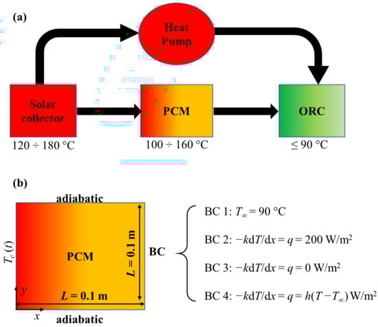
Figure 1.
The Phase Change Materials (PCM)-solar-assisted Organic Rankine Cycle (ORC) scheme: (a) sketch of the thermal system; (b) detailed boundary conditions employed in the present paper.
In this work, the maximum operating temperature assumed for the ORC fluid is about 90 °C. Thus, the outlet fluid temperature provided by the solar collector has to be in the range 100–160 °C. For this purpose, a parabolic trough solar collector (PTSC), referred to as an experimental study made in Tunisia was employed [25]. It consists of 39 m2 parabolic solar collectors made up of three modules in series, with a 19.6 geometric concentration ratio.
The collector fluid outlet temperature during the day is displayed in Figure 2, varying from about 130 °C to 160 °C, with maximum values achieved around midday, when the highest solar radiation is achieved. Sixth-order polynomial fits were employed to obtain an analytical function from experimental data from [25] to use as a boundary condition for the PCM domain.
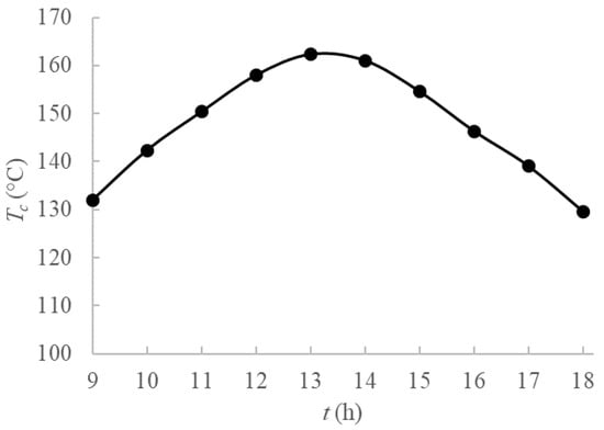
Figure 2.
Temperature profiles during the day for Tunisia heat source [25].
Erythritol is chosen as PCM because of its melting point temperature, Tm = 122 °C, so, in the range 110–130 °C, in fact, at these values, PCM is able to exploit the energy gain due to the phase change. Thermophysical properties from [26,27] are summarized in Table 1, together with melting characteristics that will be described in the following section. In this study, variation of these with temperature are considered, and their laws during phase change will be described later.

Table 1.
PCM thermophysical properties.
In order to obtain temperature profiles, velocity fields and stored energy, mass, momentum and energy equations for the PCM have to be solved. A 2D rectangular coordinate system is used in the present work, with y the coordinate that is parallel to both heated surface and gravity vector. The PCM initial temperature is below the melting point, and during the heating, the melting front moves from the heated boundary to the opposite one with a certain velocity due to liquid phase natural convection motions. A fixed grid technique is employed because the melting front is not known a priori. This characterization entails the apparent heat capacity method, which supposes proportionality of internal energy to the temperature by means of heat capacity. Furthermore, heat capacity depends on the PCM phase; energy equation for a 2D rectangular system can be written as:
where ρ is the density, u and v are the velocity components in x and y directions, respectively, and the equivalent specific heat cp,eq will be defined later.
The transient mass and momentum equations are described as:
x-momentum equation:
y-momentum equation:
where μ is the dynamic viscosity, and p is the pressure. Buoyancy effects are described by means of Boussinesq approximation for natural convection. B is a function used to achieve the gradual transition from zero velocity in the fully solid state, to a finite velocity in the fully liquid state, and it could be defined applying different methods, such as the Carman–Kozeny equations or linear functions as described in [28,29,30,31]:
where η is a very large number (107) and α(T) is the melting fraction which is equal to 0 for the fully solid state and 1 for the pure liquid and it is described as follows:
where ΔTm is the transition from solid to liquid temperature range, which is 20 °C. Generally, the melting fraction function depicted in Equation (6) is modeled by means of a linear interpolation during phase change. In this study, we use this sinusoidal function to guarantee function continuity everywhere.
Moreover, the term Fb in Equation (4) represents the buoyance force modelled through the Boussinesq approximation as:
where g is the acceleration due to gravity, β is the thermal expansion coefficient, and Tref is the temperature reference value, assumed to be the lower limit of melting point, i.e., (Tm − ΔTm/2).
As aforementioned, in this study thermophysical properties variation with temperature is considered. The specific heat for the accumulation term depends on the PCM phase, so, the specific heat curve is obtained starting from Direct Scanning Calorimetry (DSC) of the substance, taken from the literature [32]. Thus, latent heat of fusion, melting temperature, and melting temperature range ΔTm can be obtained as in [31]. The specific heat is described by the following equation:
where α(T) is the melting fraction defined in Equation (6). For the specific heat, it has been shown that there are no relevant changes with temperature during solid or liquid phases [26,33].
Thermal conductivity k and density ρ are described with the following laws that take into account the solid/liquid PCM transition via the function α(T)
where we also observe that temperature-variation of these properties when they are in single-phase can be neglected [26,33]. The same principle is applied to viscosity. Moreover, the liquid viscosity change with temperature is taken into account with the following equation, obtained by means of a non-linear regression with R2 = 0.9936 by employing data from [33]
with A = 1.592 × 10⁻⁵ Pa∙s and b = 2888 K. It is noted that the function expressed in Equation (9) is smoothed with the function α(T) during phase change, with μs = 0.0299 Pa∙s for T = Tm − ∆Tm/2. The value of μs does not affect that much the solution for the velocity field since this is forced by Equation (5).
Four different boundary conditions at the right boundary of the domain (x = L = 0.1 m) are investigated. These were previously resumed in Figure 1. For t = 0, all the solid PCM temperature is assumed to be at 100 °C. The first is a Dirichlet boundary condition (BC 1), which can occur, for example, with very high heat transfer coefficients at the right boundary of the domain. This could be the case of a two-phase flow tube that is in contact with the right part of the PCM. The second and the third (BC 2 and BC 3) are Neumann conditions, i.e., fixed heat flux and an adiabatic condition, respectively. The fixed heat flux simulates a heat storage system which allows the PCM operation, while the adiabatic condition simulates the PCM storing thermal energy during charging. Finally, the last boundary condition is a Robin one (BC 4), which simulates heat given to a fluid, for example representing the environment, which is at a slightly lower temperature than the PCM operation point. Besides, this can be also representative of a case in which heat is given to a heat exchanger, where the heat transfer coefficient generally refers to an overall heat transfer coefficient of the heat exchanger.
Moreover, at the left boundary of the domain (x = 0), the analytical function for the collector fluid outlet temperature is applied, while the top and bottom boundaries (y = 0 and y = L = 0.1 m) are considered insulated.
Governing equations are solved in COMSOL Multiphysics® (Burlington, MA, USA) with a finite element scheme. A mapped mesh of 10,000 elements is applied, and the grid convergence is verified, so using finer meshes the results do not change that much. The absolute tolerance used is 0.0005, the PARDISO direct solver is employed with the implicit free Backward Differentiation Formulas (BDF) time-stepping method with initial and maximum steps of 0.001 h and 0.1 h, respectively.
3. Results and Discussion
Results comparing the models with and without natural convection included will be presented in terms of temperature profiles and cumulated energy. Cumulated energy is obtained by performing the internal energy integration over time for two consecutive times as in [34], where the internal energy is proportional to the temperature difference via the effective specific heat capacity defined in Equation (8).
In Figure 3 a comparison between the 1D finite-difference model developed by Iasiello et al. [34] and the 2D model without natural convection of the present study is shown in terms of temperature profiles for the four boundary conditions. From the figure, the good agreement for all the cases can be confirmed. Note that in the 2D case there are no temperature gradients along the y-direction because of the boundary conditions.
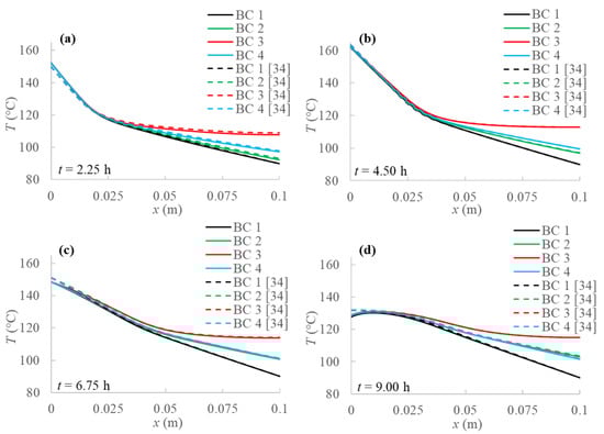
Figure 3.
Comparison between temperature profiles for the 1D model [34] and the present 2D model without natural convection at different evaluation times: (a) after 2.25 h; (b) after 4.50 h; (c) after 6.75 h; (d) after 9.00 h from the simulation beginning respectively.
From Figure 3, some considerations can be made on the temperature profiles obtained by applying the four different boundary conditions. First of all, it is shown that temperature on the left side of PCM increases in the first half of evaluation time in all cases, which is directly related to the energy provided by the sun throughout the day, as reported in Figure 2. On the other hand, the temperature drops from the second half to the end of simulations, due to the less solar energy amount. Moreover, comparing the different boundary conditions analyzed, Figure 3 clearly points out that the adiabatic condition (BC 3) results in higher temperature values than the other investigated boundary conditions. In fact, heat from the solar collector enters on the left boundary and has no exit on the right. Obviously, this boundary condition also provides the highest stored energy values.
On the other hand, the Dirichlet boundary condition (BC 1) provides lower temperature profiles and consequently stored energy since fixed temperature constrains PCM temperature growth. With reference to the other two BCs, Robin (BC 4) and Neumann (BC 2) conditions produce similar outcomes, especially as the simulation advances in time. In both cases, a slight temperature increase in time at the right side of the PCM (x = 0.1 m) can be detected, due to a larger amount of heat coming from the solar system as compared to heat going to the environment.
The results without natural convection are compared with the ones obtained including natural convection in the model. Temperature profiles are evaluated for every boundary condition studied at three different y sections of the PCM domain as shown in Figure 4, i.e., at the bottom (y = 0 m), at the middle (y = 0.05 m) and at the top (y = 0.1 m). Figure 5, Figure 6, Figure 7 and Figure 8 display temperature profiles achieved including natural convection in the model. The first general outcome to highlight in all cases is that the higher the evaluation line the higher the temperature values achieved for the entire simulation time. This is due to the buoyancy force considered in the momentum equation (Equation (4)), which takes into account the density variation with temperature, using the Boussinesq approximation, that makes liquid PCM to have a certain velocity. With references to the so-called Line 1, this line (y = 0 m) presents no relevant convection effect, while from Line 2 (y = 0.05 m) at a certain point natural convection makes temperatures higher. Another result to point out is the different heat propagation displayed, which occurs clearly not only from the left to the right side of PCM, but also from the bottom to the top of the domain, which generates convective motions as the fluid condition is achieved. Furthermore, temperature obtained in the domain are meanly higher than in the previous case analyzed without natural convection, especially considering the top of the PCM domain, this consequently results in higher cumulated energy as shown in Figure 8 and Figure 9.
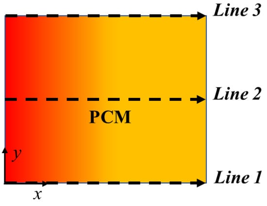
Figure 4.
Scheme of the three different PCM transversal sections: Line 1 (y = 0 m); Line 2 (y = 0.05 m); Line 3 (y = 0.1 m).
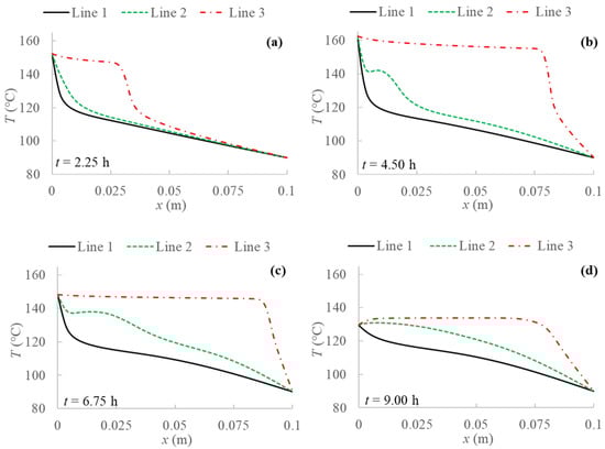
Figure 5.
Temperature profiles for 2D model with natural convection and boundary condition (BC) 1 evaluated at three different PCM transversal sections: Line 1 (y = 0 m); Line 2 (y = 0.05 m); Line 3 (y = 0.1 m), and at different evaluation times: (a) after 2.25 h; (b) after 4.50 h; (c) after 6.75 h; (d) after 9.00 h from the simulation beginning respectively.
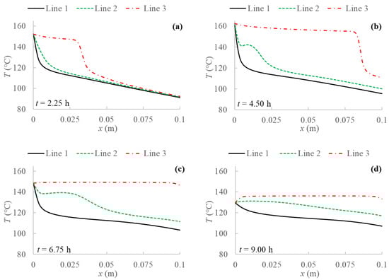
Figure 6.
Temperature profiles for 2D model with natural convection and BC 2 evaluated at three different PCM transversal sections: Line 1 (y = 0 m); Line 2 (y = 0.05 m); Line 3 (y = 0.1 m), and at different evaluation times: (a) after 2.25 h; (b) after 4.50 h; (c) after 6.75 h; (d) after 9.00 h from the simulation beginning respectively.
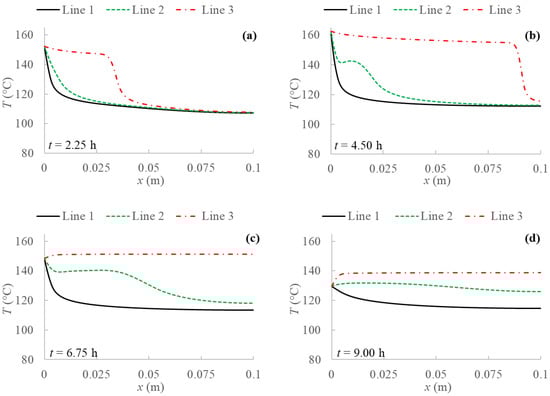
Figure 7.
Temperature profiles for 2D model with natural convection and BC 3 evaluated at three different PCM transversal sections: Line 1 (y = 0 m); Line 2 (y = 0.05 m); Line 3 (y = 0.1 m), and at different evaluation times: (a) after 2.25 h; (b) after 4.50 h; (c) after 6.75 h; (d) after 9.00 h from the simulation beginning respectively.
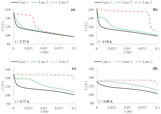
Figure 8.
Temperature profiles for 2D model with natural convection and BC 4 evaluated at three different PCM transversal sections: Line 1 (y = 0 m); Line 2 (y = 0.05 m); Line 3 (y = 0.1 m), and at different evaluation times: (a) after 2.25 h; (b) after 4.50 h; (c) after 6.75 h; (d) after 9.00 h from the simulation beginning respectively.
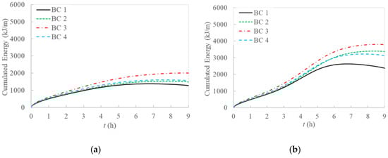
Figure 9.
Cumulated energy for 2D model: (a) without natural convection; (b) with natural convection included in the model.
Regarding the cumulated energy, Figure 9 shows that there is a high increase at the beginning of the simulation, while a maximum is reached just before the end, because the solar energy source does not provide constant temperature, thus temperature decrease could cause a heat flux inversion at the end of the transient, making the energy amount in the PCM lower. This effect is more relevant in BC 1 because of the generally lower temperatures achieved for this case.
Including natural convection, cumulated energy in the PCM domain increases are remarkable, meanly of about 52%, 63%, 48%, and 55% in the entire domain for BC 1, BC 2, BC 3, and BC 4 respectively, and up to about 100% in the second half of evaluation time, when the solar radiation decreases. This remarks on the importance of considering natural convection in these studies.
Comparing temperature profiles for the different boundary conditions, as described previously in Figure 3 without including natural convection, the adiabatic condition (BC 3) results in higher temperature values than the other investigated boundary conditions, and so the highest stored energy values. Moreover, the Dirichlet boundary condition (BC 1) provides lower temperature profiles and consequently stored energy. As regards Robin (BC 4) and Neumann (BC 2) conditions, they result in similar behaviors compared to the case without natural convection only in the first half of examination time. In the second half, instead, temperature for BC 4 is lower than for BC 2, especially at the right side of PCM and considering the central line (Line 2), as displayed in Figure 5, Figure 6, Figure 7 and Figure 8.
Figure 10, Figure 11, Figure 12 and Figure 13 show the velocity field’s evolution in time, considering the different boundary conditions analyzed. From these figures, the velocity increase in the first half of simulations is displayed for all the BCs and it confirms the previously described temperature increase. The next gradual velocity decrease in the second half of simulations is distinctly displayed too, in agreement with the decreasing fluid collector temperature profile due to the solar energy. Moreover, fluid motions from the bottom to the top, due to the buoyancy force, and from the left to right PCM side are clearly shown, confirming the results described for temperature profiles. Furthermore, the falling movements from the top to the bottom are pointed out too, highlighting the development of the convective motion as the fluid condition is obtained. Comparing the different BCs situations at the same evaluation time from Figure 10, Figure 11, Figure 12 and Figure 13, a very close behavior can be observed in the first 4.50 h among all the BCs. On the contrary, different behaviors occur in the second half of evaluation time: after 6.75 h, BC 1 and BC 4 cases give similar velocity fields, as shown in Figure 10 and Figure 13, while BC 2 results in similar outcomes to BC 3 ones, as shown in Figure 11 and Figure 12. Since the heat transfer is higher on the right boundary in BC 1 and BC 4, the velocity is higher than BC 2 and BC 3 situations, thus, the higher the heat transfer on the right boundary of PCM, the higher the fluid velocity. This can be attributed to the boundary condition referred to on the right side of the investigated PCM. Indeed, the highest velocities are achieved for BC 3, which is the adiabatic case that provides the highest values of temperature and stored energy.
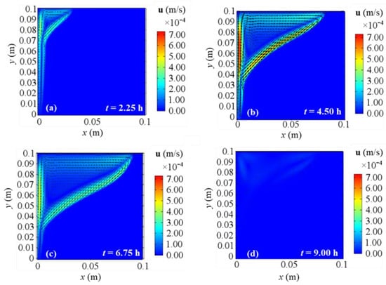
Figure 10.
Velocity fields for 2D model with natural convection and BC 1 at different evaluation times: (a) after 2.25 h; (b) after 4.50 h; (c) after 6.75 h; (d) after 9.00 h from the simulation beginning respectively.
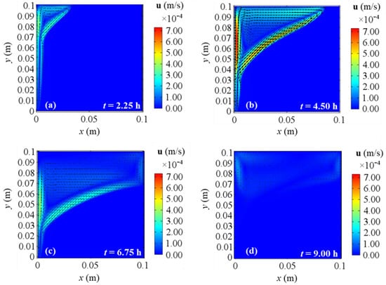
Figure 11.
Velocity fields for 2D model with natural convection and BC 2 at different evaluation times: (a) after 2.25 h; (b) after 4.50 h; (c) after 6.75 h; (d) after 9.00 h from the simulation beginning respectively.
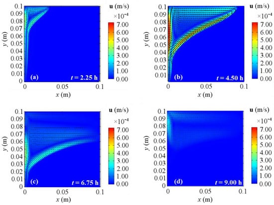
Figure 12.
Velocity fields for 2D model with natural convection and BC 3 at different evaluation times: (a) after 2.25 h; (b) after 4.50 h; (c) after 6.75 h; (d) after 9.00 h from the simulation beginning respectively.
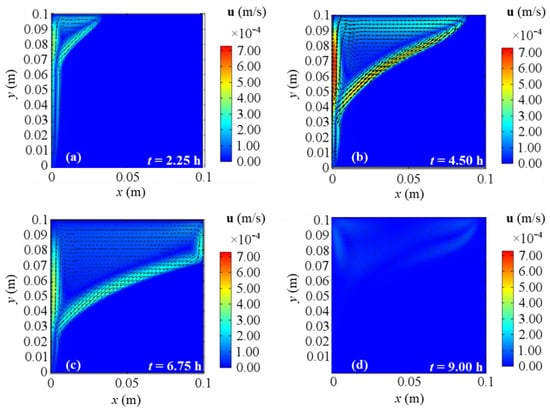
Figure 13.
Velocity fields for 2D model with natural convection and BC 4 at different evaluation times: (a) after 2.25 h; (b) after 4.50 h; (c) after 6.75 h; (d) after 9.00 h from the simulation beginning respectively.
At the end of the simulation time, first of all, one can observe a reduction of the liquid phase velocity, that arises in the third investigated time (t = 6.75 h) too. This happens because the solar collector has its peak temperature in the middle of the present analysis (see Figure 2), thus consequently liquid velocity and temperature start to drop. With references to the end of the simulation, BC 1 and BC 4 cases yield similar velocity fields, while BC 2 gives results comparable to BC 3 ones again. As aforementioned for temperature profiles, BC 1 and BC 3 result in the lowest and the highest temperature values respectively (which correspond to the lowest and the highest energy stored respectively), so again the velocity fields confirm that the higher the heat transfer on the right boundary, the lower the temperatures, and consequently the obtained cumulated energy.
As regards the phase change, Figure 14, Figure 15, Figure 16 and Figure 17 display the alpha-function evolution in time (Equation (6)), which is representative of the total melting fraction time, considering the four different boundary conditions. From these figures it is confirmed that the heat moves from the left to the right side and from the bottom to the top of PCM, causing a gradual temperature increase, that causes phase change. The bottom-to-top movement can be attributed to natural convection, while the melting fraction trend qualitatively follows velocity profiles. Moreover, the larger amount of liquid fraction at the end of the simulation is achieved for BC 3, i.e., the adiabatic condition, while BC 1 results in the lowest fluid fraction obtained, in agreement to the temperature profiles previously shown. Finally, one can also observe that the separation zone between solid and fluid clearly sets the limits of the velocity fields shown in Figure 10, Figure 11, Figure 12 and Figure 13 because of the damping function employed to characterize the momentum equation (see Equation (6)).
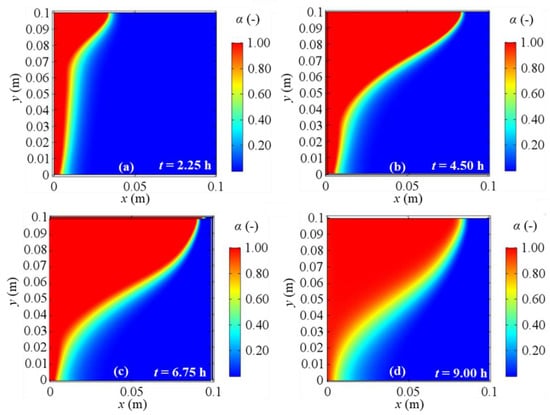
Figure 14.
Melting fraction evolution for 2D model with natural convection and BC 1 at different evaluation times: (a) after 2.25 h; (b) after 4.50 h; (c) after 6.75 h; (d) after 9.00 h from the simulation beginning respectively.
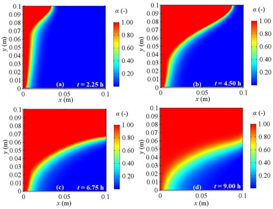
Figure 15.
Melting fraction evolution for 2D model with natural convection and BC 2 at different evaluation times: (a) after 2.25 h; (b) after 4.50 h; (c) after 6.75 h; (d) after 9.00 h from the simulation beginning respectively.
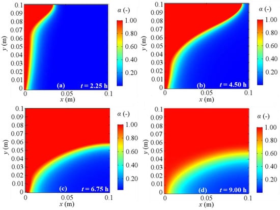
Figure 16.
Melting fraction evolution for 2D model with natural convection and BC 3 at different evaluation times: (a) after 2.25 h; (b) after 4.50 h; (c) after 6.75 h; (d) after 9.00 h from the simulation beginning respectively.
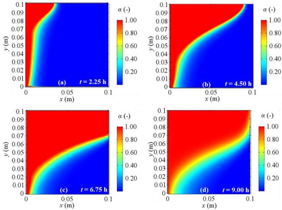
Figure 17.
Melting fraction evolution for a 2D model with natural convection and BC 4 at different evaluation times: (a) after 2.25 h; (b) after 4.50 h; (c) after 6.75 h; (d) after 9.00 h from the simulation beginning respectively.
4. Conclusions
In this work, a solar-assisted PCM used for ORC energy storage was numerically studied employing the apparent heat capacity method for the energy equation, including natural convection effects by means of the Boussinesq approximation term in the momentum equation. A damping function is used in the momentum equation in order to solve velocity field everywhere, with negligible values when PCM is in the solid phase. Four different boundary conditions at the PCM/ORC interface refer to uniform and constant temperature, heat flux or convective heat flux, or to adiabatic conditions, were investigated. The solar source was modeled with a time-variable temperature boundary condition, according to experimental data from the literature. Results are presented in terms of temperature profiles, velocity fields, melting fraction and stored energy, showing differences in including or not natural convection effects in the model.
The outcomes show that the higher the solar source temperature the higher the temperature and the stored energy of the system, as expected. Furthermore, natural convection effects are remarkable on the temperature values and consequently stored energy achieved. In fact, including natural convection, the cumulated energy in the PCM domain increases are remarkable, meanly of about 45%, 61%, 51%, and 56% in the entire domain for BC 1, BC 2, BC 3, and BC 4 respectively, and up to about 100% in the second half of evaluation time, when the solar radiation decreases. In addition, the velocity fields confirm that the higher the heat transfer on the right boundary, the lower the temperatures, and consequently the obtained cumulated energy.
Author Contributions
Conceptualization, A.A., M.I., and C.T.; methodology, A.A., M.I., and C.T.; software, M.I. and C.T.; validation, M.I. and C.T.; formal analysis, A.A., M.I., and C.T.; investigation, A.A., M.I., and C.T.; resources, A.A., M.I., and C.T.; data curation, A.A., M.I., and C.T.; writing—original draft preparation, M.I. and C.T.; writing—review and editing, A.A., M.I., and C.T.; visualization, A.A., M.I., and C.T; supervision, A.A.; project administration, A.A.; funding acquisition, A.A. All authors have read and agreed to the published version of the manuscript.
Funding
This work was supported by the Italian Government MIUR Grant N° “PRIN-2017F7KZWS”.
Institutional Review Board Statement
Not applicable.
Informed Consent Statement
Not applicable.
Data Availability Statement
No new data were created or analyzed in this study. Data sharing is not applicable to this article.
Conflicts of Interest
The authors declare no conflict of interest.
Nomenclature
| B | Solid-liquid transition function (-) |
| cp | Specific heat capacity (J/kg K) |
| Fb | Buoyance force term (N/m3) |
| g | Acceleration due to gravity (m/s2) |
| h | Heat transfer coefficient (W/m2 K) |
| k | Thermal conductivity (W/m K) |
| L | Length (m) |
| p | Pressure (Pa) |
| q | Heat flux (W/m2) |
| t | Time (s) |
| T | Temperature (°C) |
| u | horizontal velocity component (m/s) |
| v | vertical velocity component (m/s) |
| x | Spatial coordinate (m) |
| y | Spatial coordinate (m) |
| Greek symbols | |
| α | Alpha function (-) |
| β | Thermal expansion coefficient (1/K) |
| λ | Latent heat of fusion (J/kg) |
| ΔTm | Transition from solid to liquid temperature range (K) |
| η | Large constant |
| μ | Dynamic viscosity (kg/m s) |
| ρ | Density (kg/m3) |
| Subscripts | |
| ∞ | Environment |
| c | Collector |
| eq | Equivalent |
| l | Liquid PCM |
| m | Melting |
| ref | Reference |
| s | Solid PCM |
References
- Wang, M.; Wang, J.; Zhao, Y.; Zhao, P.; Dai, Y. Thermodynamic analysis and optimization of a solar-driven regenerative Organic Rankine Cycle (ORC) based on flat-plate solar collectors. Appl. Eng. 2013, 50, 816–825. [Google Scholar] [CrossRef]
- Franco, A. Power production from a moderate temperature geothermal resource with regenerative Organic Rankine Cycles. Energy Sustain. Dev. 2011, 15, 411–419. [Google Scholar] [CrossRef]
- Algieri, A.; Morrone, P. Comparative energetic analysis of high-temperature subcritical and transcritical Organic Rankine Cycle (ORC). A biomass application in the Sibari district. Appl. Eng. 2012, 36, 236–244. [Google Scholar] [CrossRef]
- Aussant, C.D.; Fung, A.S.; Ugursal, V.I.; Taherian, H. Residential application of internal combustion engine-based cogeneration in cold climated Canada. Energy Build. 2009, 41, 1288–1298. [Google Scholar] [CrossRef]
- Dolz, V.; Novella, R.; García, A.; Sanchez, J. HD diesel engine equipped with a bottoming Rankine cycle as a waste heat recovery system. Part 1: Study and analysis of the waste heat energy. Appl. Eng. 2012, 36, 269–278. [Google Scholar] [CrossRef]
- Wang, D.; Ling, X.; Peng, H. Performance analysis of double Organic Rankine Cycle for discontinuous low temperature waste heat recovery. Appl. Eng. 2012, 48, 63–71. [Google Scholar] [CrossRef]
- Wang, H.; Peterson, R.; Herron, T. Design study of configurations on system COP for a combined ORC (Organic Rankine Cycle) and VCC (vapor compression cycle). Energy 2011, 36, 4809–4820. [Google Scholar] [CrossRef]
- Zhou, D.; Zhao, C.Y.; Tian, Y. Review on thermal energy storage with phase change materials (PCMs) in building applications. Appl. Energy 2012, 92, 593–605. [Google Scholar] [CrossRef]
- Zalba, B.; Marìn, J.M.; Cabeza, L.F.; Mehling, H. Review on thermal energy storage with phase change: Materials, heat transfer analysis and applications. Appl. Therm. Eng. 2003, 23, 251–283. [Google Scholar] [CrossRef]
- Wang, S.; Baldea, M. Temperature control and optimal energy management using latent energy storage. Ind. Eng. Chem. Res. 2013, 52, 3247–3257. [Google Scholar] [CrossRef]
- Fan, L.; Khodadadi, J.M. Thermal conductivity enhancement of phase change materials for thermal energy storage: A review. Renew. Sustain. Energy Rev. 2011, 15, 24–46. [Google Scholar] [CrossRef]
- Nakhchi, M.E.; Esfahani, J.A. Improving the melting performance of PCM thermal energy storage with novel stepped fins. J. Energy Storage 2020, 30, 101424. [Google Scholar] [CrossRef]
- Yıldız, C.; Arıcı, M.; Nižetić, S.; Shahsavar, A. Numerical investigation of natural convection behavior of molten PCM in an enclosure having rectangular and tree-like branching fins. Energy 2020, 207, 118223. [Google Scholar] [CrossRef]
- Agyenim, F. The use of enhanced heat transfer phase change materials (PCM) to improve the coefficient of performance (COP) of solar powered LiBr/H2O absorption cooling systems. Renew. Energy 2016, 87, 229–239. [Google Scholar] [CrossRef]
- Rostami, S.; Afrand, M.; Shahsavar, A.; Sheikholeslami, M.; Kalbasi, R.; Aghakhani, S.; Shadloo, M.S.; Oztop, H.F. A review of melting and freezing processes of PCM/nano-PCM and their application in energy storage. Energy 2020, 211, 118698. [Google Scholar] [CrossRef]
- Ghasemiasl, R.; Hoseinzadeh, S.; Javadi, M.A. Numerical Analysis of Energy Storage Systems Using Two Phase-Change Materials with Nanoparticles. J. Thermophys. Heat Transf. 2018, 32, 440–448. [Google Scholar] [CrossRef]
- Hoseinzadeh, S.; Ghasemiasl, R.; Havaei, D.; Chamkha, A.J. Numerical investigation of rectangular thermal energy storage units with multiple phase change materials. J. Mol. Liq. 2018, 271, 655–660. [Google Scholar] [CrossRef]
- Mosaffa, A.H.; Talati, F.; Tabrizi, H.B.; Rosen, M.A. Analytical modeling of PCM solidification in a shell and tube finned thermal storage for air conditioning systems. Energy Build. 2012, 49, 356–361. [Google Scholar] [CrossRef]
- Kargar, M.R.; Baniasadi, E.; Mosharaf-Dehkordi, M. Numerical analysis of a new thermal energy storage system using phase change materials for direct steam parabolic trough solar power plants. Sol. Energy 2018, 170, 594–605. [Google Scholar] [CrossRef]
- Qi, R.; Wang, Z.; Ren, J.; Wu, Y. Numerical investigation on heat transfer characteristics during melting of lauric acid in a slender rectangular cavity with flow boundary condition. Int. J. Heat Mass Transf. 2020, 157, 119927. [Google Scholar] [CrossRef]
- Jurćević, M.; Penga, Ž.; Klarin, B.; Nižetić, S. Numerical analysis and experimental validation of heat transfer during solidification of phase change material in a large domain. J. Energy Storage 2020, 30, 101543. [Google Scholar] [CrossRef]
- Gürel, B. A numerical investigation of the melting heat transfer characteristics of phase change materials in different plate heat exchanger (latent heat thermal energy storage) systems. Int. J. Heat Mass Transf. 2020, 148, 119117. [Google Scholar] [CrossRef]
- Hajjar, A.; Mehryan SA, M.; Ghalambaz, M. Time periodic natural convection heat transfer in a nano-encapsulated phase-change suspension. Int. J. Mech. Sci. 2020, 166, 105243. [Google Scholar] [CrossRef]
- Cataldo, F.; Mastrullo, R.; Mauro, A.W.; Vanoli, G.P. Fluid selection of Organic Rankine Cycle for low-temperature waste heat recovery based on thermal optimization. Energy 2014, 72, 159–167. [Google Scholar] [CrossRef]
- Balghouthi, M.; Ali AB, H.; Trabelsi, S.E.; Guizani, A. Optical and thermal evaluations of a medium temperature parabolic trough solar collector used in a cooling installation. Energy Convers. Manag. 2014, 86, 1134–1146. [Google Scholar] [CrossRef]
- Höhlein, S.; König-Haagen, A.; Brüggemann, D. Thermophysical Characterization of MgCl2·6H2O, Xylitol and Erythritol as Phase Change Materials (PCM) for Latent Heat Thermal Energy Storage (LHTES). Materials 2017, 10, 444. [Google Scholar] [CrossRef] [PubMed]
- Kaizawa, A.; Kamano, H.; Kawai, A.; Jozuka, T.; Senda, T.; Maruoka, N.; Akiyama, T. Thermal and flow behaviors in heat transportation container using phase change material. Energy Convers. Manag. 2008, 49, 698–706. [Google Scholar] [CrossRef]
- Voller, V.R.; Cross, M.; Markatos, N.C. An enthalpy method for convection/diffusion phase change. Int. J. Numer. Methods Eng. 1987, 24, 271–284. [Google Scholar] [CrossRef]
- Brent, A.D.; Voller, V.R.; Reid, K.T.J. Enthalpy-porosity technique for modeling convection-diffusion phase change: Application to the melting of a pure metal. Numer. Heat Transf. Part A Appl. 1988, 13, 297–318. [Google Scholar]
- Sciacovelli, A.; Colella, F.; Verda, V. Melting of PCM in a thermal energy storage unit: Numerical investigation and effect of nanoparticle enhancement. Int. J. Energy Res. 2013, 37, 1610–1623. [Google Scholar] [CrossRef]
- Yang, H.; Zhang, H.; Sui, Y.; Yang, C. Numerical analysis and experimental visualization of phase change material melting process for thermal management of cylindrical power battery. Appl. Therm. Eng. 2018, 128, 489–499. [Google Scholar] [CrossRef]
- Ji, H.; Sellan, D.P.; Pettes, M.T.; Kong, X.; Ji, J.; Shi, L.; Ruoff, R.S. Enhanced thermal conductivity of phase change materials with ultrathin-graphite foams for thermal energy storage. Energy Environ. Sci. 2014, 7, 1185–1192. [Google Scholar] [CrossRef]
- Wang, Y.; Wang, L.; Xie, N.; Lin, X.; Chen, H. Experimental study on the melting and solidification behavior of erythritol in a vertical shell-and-tube latent heat thermal storage unit. Int. J. Heat Mass Transf. 2016, 99, 770–781. [Google Scholar] [CrossRef]
- Iasiello, M.; Braimakis, K.; Andreozzi, A.; Karellas, S. Thermal analysis of a Phase Change Material for a Solar Organic Rankine Cycle. J. Phys. Conf. Ser. 2017, 923, 012042. [Google Scholar] [CrossRef]


Publisher’s Note: MDPI stays neutral with regard to jurisdictional claims in published maps and institutional affiliations. |
© 2021 by the authors. Licensee MDPI, Basel, Switzerland. This article is an open access article distributed under the terms and conditions of the Creative Commons Attribution (CC BY) license (http://creativecommons.org/licenses/by/4.0/).