Thermal Resistance Matrix Extraction from Finite-Element Analysis for High-Frequency Magnetic Components

Abstract

The thermal management of magnetic components for power electronics is crucial to ensure their reliability. However, conventional thermal models for magnetic components are known to have either poor accuracy or excessive complexity. Contrary to these models, the use of Thermal Resistance Matrices is proposed in this paper instead, which combine both accuracy and simplicity. They are usually used to characterize semiconductor devices, but not for magnetic components. The guidelines to apply Thermal Resistance Matrices for magnetic components are discussed in detail. The accuracy of this model is validated by 3D FEA simulations and experimental results, showing an absolute error lower than 5 ${}^{\circ }$C and a relative error between $-6.4\%$ and $3.9\%$, which is outstanding compared to the carried-out literature review.

1. Introduction

The constantly increasing interest in miniaturising power components makes crucial a proper characterisation of the thermal behaviour of magnetic components, which are one of the limiting factors [1,2].

The simplest and most widely used approach is the empirical Equation (1) from [3], or other simple equations like the one proposed in [4]. Nevertheless, their accuracy is considerably limited, while it serves as a first order approximation.

$$R_{th}=53·V_e^{-0.54}$$

(1)

Another recurrent approach is to use thermal networks for magnetic components [5,6,7] (or for semiconductors [8]), which shows better results than Equation (1). Their accuracy is associated with their granularity, hence to their complexity, which is still limited since a constant film coefficient is commonly assumed. To compensate this fact, some authors model the fluid dynamics by means of non-linear resistances [9,10,11,12], which add extra complexity to the model.

Different approaches consist of building a model based on experimental results, explained in [13,14], or using an inverse model in which the correction of some analytical equations is made by means of prototype results [15]. However, they both have the inherent drawback of requiring a prototype and their application is limited to the boundary conditions of the experiments [16].

In this article, the use of thermal resistance matrices for magnetic components is proposed. Some applications of this model to semiconductors can be found in [17,18,19]. This approach offers several advantages compared to the previous ones. This model consists of a simple coefficients matrix of dimension N × N, where N is the number of characterised objects or parts (for example, the core, the windings and the bobbin). This matrix characterizes the temperature at each part, accounting for the self heating effects as well as the mutual heating between each part. Additionally, regardless of the heterogeneity of the device or the complexity of the boundary conditions, the thermal resistance matrix captures the thermal behaviour of the device very accurately.

As an example, the temperature rise of an E25/13/7 transformer predicted by 3D Finite Element Analysis (FEA) simulations for a range of winding power losses with constant core losses. This is illustrated in Figure 1 along with the results obtained by using Equation (1) and the proposed thermal resistance matrix. It can be seen that the last one shows considerably better results.

2. Proposed Model

The accuracy of 3D FEA simulations, as well as their capability to analyze complex systems, allows the obtaining of a static FEA-based thermal model to estimate the temperature of any object within a system under any operating point [20]. Furthermore, any boundary condition can be recreated by simulation, regardless of their nature or complexity [21,22].

While the concept of a thermal resistance matrix is generic, some special concerns need to be considered when applying it to magnetic components, which are discussed next.

2.1. Modeling Transformers and Inductors

A step-by-step guide to obtain a thermal resistance matrix to characterize any magnetic component is explained along this section. A flow diagram of the corresponding procedure steps is depicted in Figure 2, as a summary of the proposed methodology.

2.1.1. Representative Objects in a Magnetic Component

The first step consists of splitting the magnetic component in the least amount of representative objects. In other words, since a thermal resistance matrix of dimension N × N characterizes the interaction between N objects, there is an accuracy-complexity compromise in the model. The main ‘objects’ to be characterised are described next:

• Magnetic core: its temperature rise is crucial to analyze its magnetic behaviour (permeability and saturation flux).
• Main windings: windings with considerably different physical characteristics (geometry, materials, power losses) can be treated as separate objects for higher accuracy or together to reduce N for simplicity.
• Auxiliary windings: whereas their power losses are negligible, they can be treated as an additional object if their temperature is relevant for the analysis.
• Passive parts: a coil former or the pin connectors to a PCB do not have power losses, but their temperature depends on the heat flux coming from surrounding objects, which could be critical if the maximum ratings are exceeded.

2.1.2. Linearization

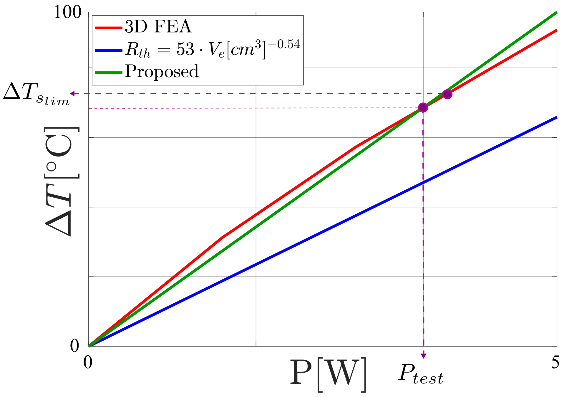
In order to build a thermal resistance matrix, the superposition principle must be applied, which is only possible in linear systems. However, only the thermal conduction is linear while convection and radiation are non-linear [23,24]. This effect is shown in Figure 1, where the temperature rise of a certain magnetic core, exposed to natural convection and radiation, is depicted for different power losses. Contrary to semiconductors, where the conductive heat transfer is dominant due to their reduced size and encapsulation, the evolution of this temperature rise is clearly non-linear because the magnetic components are more exposed to convection and radiation.

Therefore, the system must be linearized and a proper thermal operating point must be selected since the slope of the linearized ‘resistance’ will change accordingly. To achieve realistic results, the thermal operating point must be equal (or close) to the limit temperature rise of the corresponding object, $\Delta T_{s_{lim}}$ (see Figure 1). Each object can have a different $\Delta T_{s_{lim}}$, depending on the materials and the specifications of the project.

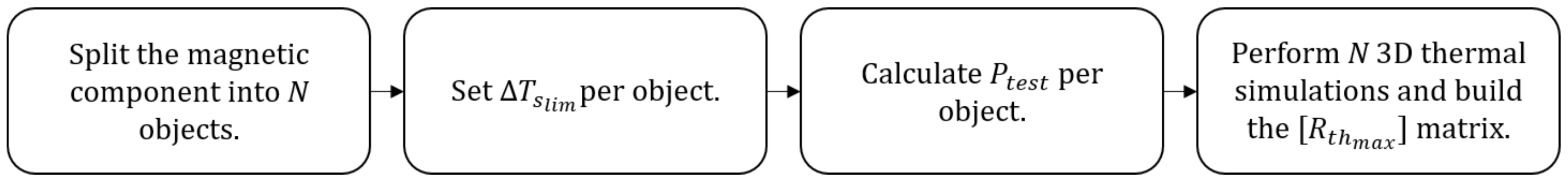
By chosing this $\Delta T_{s_{lim}}$ for each object, a value of power losses per object will be calculated so that a thermal resistance per object can be obtained to characterise its temperature rise from $T_{amb}$ to $\Delta T_{s_{lim}}$—assuming a linear behaviour—, as explained in the following steps.

As a summary, this steps consists only in choosing the maximum allowed (or limit) temperature rise, $\Delta T_{s_{lim}}$, for each object.

2.1.3. $P_{test}$ Calculation for the Magnetic Core, the Windings and the Passive Objects

The thermal resistance is equal to the temperature rise divided by the power losses (or heat) flowing through an object if the system is linear, according to [23,24]. To obtain that thermal resistance, certain test power losses ($P_{test}$, in Watts) are injected and the subsequent temperature rise is measured. For semiconductors, a common choice consists of making $P_{test}$ equal to the maximum rated power of the device, given by the manufacturers.

However, selecting $P_{test}$ for each part of a magnetic component is not obvious due to the non-linear behaviour explained in the previous step. As the temperature rise of each object must be equal (or close) to its $\Delta T_{s_{lim}}$, the value of $P_{test}$ must be selected accordingly. Two methods can be used to obtain $P_{test}$: by trial and error in simulation, which is time-consuming and therefore not recommended, or using basic heat transfer equations and some geometrical approximations, which is explained next.

For the magnetic core, $P_{test}$ is calculated in Equation (2) using the convection and radiation expressions from the external surfaces of the core to the ambient, which are defined in Equations (3) and (4), respectively:

$$P_{test}=Q_{conv}+Q_{rad}$$

(2)

$$Q_{conv}=\sum _s\left(h_s·A_s·\Delta T_{s_{lim}}\right)$$

(3)

$$Q_{rad}=ϵ·\sum _s{A}_s·\sigma ·(T_{s_{lim}}^4-T_{amb}^4),$$

(4)

where $Q_{conv}$ and $Q_{rad}$ are the heat transferred by convection and radiation (in Watts), respectively; $A_s$ is the external heat exchange surface exposed to the ambient, in squared meters; $ϵ$ is the relative emissivity of the object; $\sigma$ is the Stefan-Boltzmann constant ($5.670373\times {10}^{-8}\frac{W}{m^2·K^4}$); and $h_s$ is the film factor coefficient corresponding to each surface, in W/m${}^2·$K. The ambient temperature ($T_{amb}$) and $T_{s_{lim}}$ must be expressed in Kelvin.

The typical film factors for natural convection are shown in

Table 1. Film coefficient for natural convection for typical geometries [23,24].

Object	Film Coefficient
Vertical plate or cylinder	$h_S=1.42·{\left(\frac{\Delta T_{S_{lim}}}{L}\right)}^{0.25}$ W/m${}^2·$ K; L = height in m
Horizontal cylinder	$h_S=1.32·{\left(\frac{\Delta T_{S_{lim}}}{D}\right)}^{0.25}$ W/m${}^2·$ K; D = diameter in m
Horizontal plate hot surface down	$h_S=0.59·{\left(\frac{\Delta T_{S_{lim}}}{L}\right)}^{0.25}$ W/m${}^2·$ K; $L=\frac{4·Area}{perimeter}$ in m

. The surfaces in contact with a PCB, which are considered adiabatic, are neglected in this step. However, if the cooling capability of heatsinks and/or forced convection are considered, a simplified film factor must be calculated for each surface according to [23,24,25].

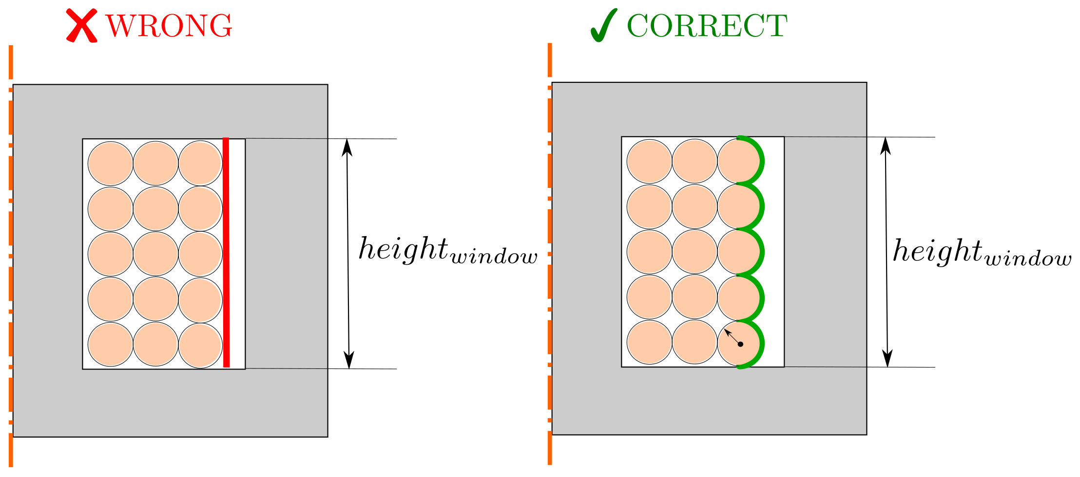
On the other hand, the windings of the magnetic components are treated as a group since only the wires in the outer layer are in direct contact with ambient. Then, the whole winding is treated as a vertical cylinder (Table 1), but the external surface of each wire must also be considered in the total heat exchange area, as highlighted in Figure 3. If the external surface of the winding is assumed to be equal to the window height, as expressed in Equation (5), the results would not be accurate. Therefore, the surface of each wire must be considered, leading to the proper external surface value in squared meters, calculated in Equation (6).

$$A_{ext}=(2·r·n_{wires})·peri{m}_{wind}$$

(5)

$$A_{ext}=(\pi ·r·n_{wires})·peri{m}_{wind},$$

(6)

where $n_{wires}$ is the number of wires in the external layer of conductors, r is their radius and $peri{m}_{wind}$ is the perimeter of that layer. In case the winding is made of litz bundles, homogenization techniques can be used to simplify them [26,27].

Since only the external layer of conductors is directly exposed to the ambient, all the windings must be treated as a block in order to calculate the required $P_{test}$, according to Equations (2)–(4). In order to simplify the calculations, it is assumed that the same $P_{test}$ is applied to all the windings:

$$P_{tes{t}_{pri}}=P_{tes{t}_{sec}}=\dots =P_{tes{t}_{wind}}$$

(7)

Finally, the power losses in the auxiliary windings are usually negligible compared to the main windings. Therefore, they can be considered as passive objects, for which $P_{test}$ is not calculated. This is also applicable for the bobbin or the pin connectors to the PCB.

2.1.4. Superposition

Once $\Delta T_{s_{lim}}$ and $P_{test}$ are calculated for every object, the next step is to identify which simulations are required to characterize the complete system.

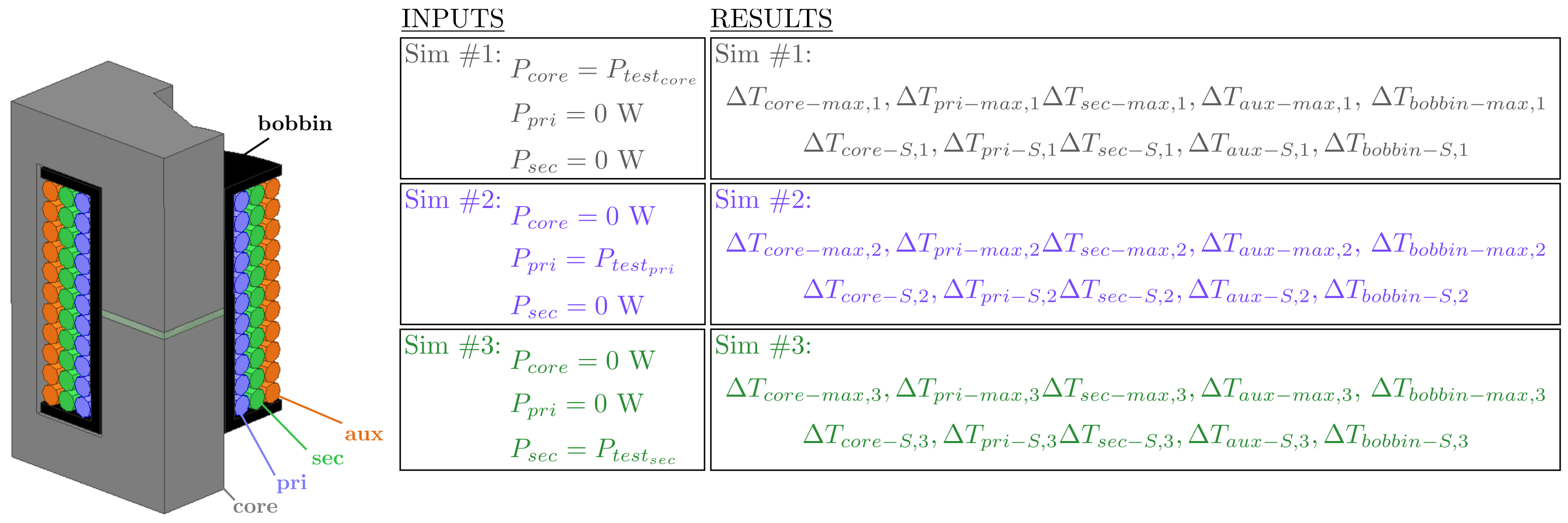
The generic transformer from Figure 4 is considered as an example. It is constituted by five objects ($N=5$): the magnetic core, a plastic bobbin and three windings (primary, secondary and auxiliary). Therefore, the corresponding thermal resistance matrix (in ${}^{\circ }$C/W) is defined next:

$$\left[R_{t{h}_{max}}\right]=\left(\begin{array}{ccccc}{\displaystyle \frac{\Delta T_{core,1}}{P_{tes{t}_{core}}}}& {\displaystyle \frac{\Delta T_{core,2}}{P_{tes{t}_{pri}}}}& {\displaystyle \frac{\Delta T_{core,3}}{P_{tes{t}_{sec}}}}& 0& 0\\ \frac{\Delta T_{pri,1}}{P_{tes{t}_{core}}}& {\displaystyle \frac{\Delta T_{pri,2}}{P_{tes{t}_{pri}}}}& {\displaystyle \frac{\Delta T_{pri,3}}{P_{tes{t}_{sec}}}}& 0& 0\\ \frac{\Delta T_{sec,1}}{P_{tes{t}_{core}}}& {\displaystyle \frac{\Delta T_{sec,2}}{P_{tes{t}_{pri}}}}& {\displaystyle \frac{\Delta T_{sec,3}}{P_{tes{t}_{sec}}}}& 0& 0\\ \frac{\Delta T_{aux,1}}{P_{tes{t}_{core}}}& \frac{\Delta T_{aux,2}}{P_{tes{t}_{pri}}}& \frac{\Delta T_{aux,3}}{P_{tes{t}_{sec}}}& 0& 0\\ \frac{\Delta T_{bobbin,1}}{P_{tes{t}_{core}}}& \frac{\Delta T_{bobbin,2}}{P_{tes{t}_{pri}}}& \frac{\Delta T_{bobbin,3}}{P_{tes{t}_{sec}}}& 0& 0\end{array}\right)$$

(8)

$\left[R_{t{h}_{max}}\right]$ is built by applying the superposition principle because the system has been previously linearized. Each column contains the maximum temperature rise of each object, normalized by the corresponding $P_{test}$. On the other hand, the auxiliary winding and the plastic bobbin have no power losses associated, so their corresponding columns (4th and 5th) are filled with zeros. However, these columns must be included in the matrix in order to calculate the maximum temperature of all the objects in the last step of the design process. The diagonal terms of this matrix ($i=j$, being i and j the indexes for the rows and the columns, respectively) represent the self-heating behaviour of each object due to the internal heat generation, while the remaining terms ($i\ne j$) express the mutual heat flux between each object.

As a conclusion, only one simulation per active object (objects with power losses) is required to obtain the temperature of every object for the calculated $P_{test}$. In this example, three simulations must be performed, as shown in Figure 4. The calculated $P_{test}$ in the previous step are assigned to a single object in each simulation. The subsequent maximum temperature rise per object from that simulation is then stored to obtain the corresponding column of $\left[R_{t{h}_{max}}\right]$ until the matrix is complete.

2.1.5. Using the Model to Estimate the Maximum Temperature Per Object

The combination of the power losses (in Watts) applied in each object, $\left[P_{loss}\right]$, is defined as a vector in Equation (9). The maximum temperature of each part of the magnetic component (in ${}^{\circ }$C) is calculated in Equation (10) by multiplying the thermal coefficients matrix, $\left[R_{t{h}_{max}}\right]$, by any combination of power losses applied in each object, $\left[P_{loss}\right]$.

$$\left[P_{loss}\right]={[P_{core},P_{pri},P_{sec},P_{aux},P_{bobbin}]}^T$$

(9)

$$\left(\begin{array}{c}\Delta T_{cor{e}_{max}}\\ \Delta T_{pr{i}_{max}}\\ \Delta T_{se{c}_{max}}\\ \Delta T_{au{x}_{max}}\\ \Delta T_{bobbi{n}_{max}}\end{array}\right)=\left[R_{t{h}_{max}}\right]·\left[P_{loss}\right]$$

(10)

It is important to notice that once $\left[Rt{h}_{max}\right]$ is built, the only input required to calculate the temperature at any region of the magnetic component is $\left[P_{loss}\right]$. This leads to a versatile model that is valid to calculate the temperature of the component for any $\left[P_{loss}\right]$ input, which means for any electrical operating point.

A generic multi-winding transformer is used as an example in this section, but the model can also be applied to inductors. They are just a particular case with just one winding, so the process to obtain $\left[Rt{h}_{max}\right]$ is identical.

2.2. Impact and Limitations

The main advantages and the scope of the developed model can be summarized next:

• It can be extended to N objects, whose behaviour will be represented in the thermal coefficients matrix.
• The self-heating effects, as well as the mutual heat flux between objects, are modelled by this simple matrix, avoiding the unfeasible complexity of the three-dimensional heat transfer equations for such heterogeneous systems as magnetic components [23,24].
• The maximum temperature can be calculated by the proposed matrix for any combination of power losses of the magnetic component.
• It is valid for any boundary conditions as long as they can be reproduced in the required simulations.
• The accuracy is ensured for temperatures around $T_{s_{lim}}$, which will be proven in Section 3. As a consequence, it allows us to properly identify the actual thermal limits of the device under test (DUT).
• The accuracy is not limited by (nor dependent on) the location of the maximum temperature per component. This is because the matrix is obtained using the maximum temperature per component, not the temperature at certain coordinates from the geometry.

Despite the wide scope and applicability of the proposed approach, it has some limitations:

• Since the behaviour of the temperature rise is assumed linear from $T_{amb}$ to $T_{s_{lim}}$, the accuracy is very high around those temperatures, but it is lower for temperatures in the middle of that range.
• The developed model is only valid for the boundary conditions (convection and radiation) established in the simulations. Therefore, a new thermal coefficients matrix must be calculated for different boundary conditions, but it can be easily obtained by changing the parameters in the simulations.
• The accuracy for temperatures higher than $T_{s_{lim}}$ is not guaranteed since the linearization of the thermal coefficients matrix is performed from $T_{amb}$ to $T_{s_{lim}}$.

3. Experimental Validation

The proposed FEA-based thermal coefficients matrix is validated along this section. First, the electrical setup and the DUT are described. Then, some aspects concerning the required simulations and the generated models are discussed. Finally, the estimated temperature rise of the tested magnetics calculated by means of this model is compared with the thermal measurements and the 3D FEA simulation results. The used simulator is ‘Icepak’, from ‘ANSYS Electronics Desktop 2019 R2’.

3.1. Experimental Setup and Tested Devices

The electrical setup is depicted in Figure 5, in which an AC current is injected into the winding of the prototypes to generate core and winding power losses, causing certain temperature rise as a consequence. First, a sinusoidal voltage waveform is generated at certain frequency by a waveform generator (GW Instek, model AFG-2005) to supply the circuit, and it is amplified by means of an RF amplifier (AR, model 150A 100B). The value of the capacitor $C_{res}$ is selected so that the resonant frequency between itself and the magnetic component under test corresponds to the input signal frequency. This capacitor is placed in series with the inductor, but in parallel with the primary winding of the transformer. This way, the impedance of the resonant tank is low enough to achieve a relatively high input current with a relatively low input voltage in both cases, avoiding the saturation of the RF amplifier due to its limited voltage gain. Since the voltage is imposed by the RF amplifier, a variable resistor ($R_{damp}$ in series for the inductor; $R_{load}$ in the secondary of the transformer) is placed in order to adjust the demanded current by the circuit. This way, the voltage and current amplitudes can be selected as desired. Since the power losses in the auxiliary winding of the transformer are assumed negligible, no load is connected to that winding.

The values of every component and the operating conditions and the characteristics of the tested prototypes are summarized in

Table 2. Components and operating conditions of the prototypes.

	A	B
$C_{res}$	3.3 nF × 2	4.7 nF × 3
L/$L_m$/$L_{lk}$	500 μH/–/–	–/169 μH/830 nH
R	0.5 $\mathsf{\Omega }$	1.8 $\mathsf{\Omega }$
$V_{pk-pk}$	976.6 V	104.7 V
$I_{pk-pk}$	2.26 A	5.19 A
$freq$	175 kHz	340 kHz
$T_{amb}$	26 ${}^{\circ }$C	26 ${}^{\circ }$C

and

Table 3. Description of the tested prototypes.

Prototype	A (Inductor)	B (Transformer)
Core	P36/22	E25/13/7
Diameter (gauge)	1 mm (AWG19)	0.81 mm (AWG21)
Gap	0.44 mm	None
Number of turns	30	9:20:10
$T_{amb}$	26 ${}^{\circ }$C	26 ${}^{\circ }$C

, respectively.

A generic inductor and a generic transformer with three windings (primary, secondary and auxiliary) with different core shapes, wire diameter and number of turns are chosen as representative samples in order to cover the scope of the proposed model. They are shown in Figure 6 along with the required resonant capacitors for the electrical setup. The thermal conductivity assumed for each material is also summarized in

Table 4. Thermal conductivity of each material assumed in this study.

	Thermal Conductivity
Ferrite core [28]	4 W/m·K
Copper conductor [29]	380 W/m·K
Bobbin [29]	$0.2$ W/m·K
Air [29]	$0.03$ W/m·K
FR4 PCB [29]	$0.25$ W/m·K
Wooden table [29]	$0.17$ W/m·K

. The emissivity have been assumed equal to 0.8 for all surfaces.

Regarding the thermal measurements, an OEM-PLUS Series optics fibre thermometer [30] is used to measure temperatures approximately located in the hot-spots, according to the cross-section representation of the prototypes from Figure 7. Then, these temperatures are used as a reference for the maximum temperatures.

3.2. Model Extraction from FEA Simulations

At this point, the procedure to obtain $\left[R_{t{h}_{max}}\right]$ for both prototypes, described in Section 2.1, is carried out. The ambient temperature of the simulations is set equal to the experiments ($T_{amb}$ = 26 ${}^{\circ }$C). The limit surface temperature is established as $T_{s_{lim}}=100$ ${}^{\circ }$C, resulting in a temperature rise of $\Delta T_{s_{lim}}=74$ ${}^{\circ }$C, which is used to calculate $P_{test}$ for each object. The values of $P_{test}$ for both prototypes are summarized in

Table 5. Values of $P_{test}$ to model the prototypes.

	A	B
Core	4.493 W	1.721 W
Main winding	2.171 W	-
Primary winding	-	1.622 W
Secondary winding		1.622 W

, considering natural convection and radiation, as well as including the PCB and the wooden table below the core of the magnetics.

The fluid dynamics of the surrounding air, as well as the radiation effects and the surrounding objects (the PCB and the table, whose material properties are defined in Table 4), are simulated in order to recreate the same conditions in the simulations as in the experimental setup. Therefore, the external faces of the boundary box must be defined as ‘openings’ in ANSYS, and both convection and radiation must be enabled.

The obtained thermal coefficients matrix (in ${}^{\circ }$C/W) for the inductor (object A) is shown next, being core and winding the objects 1 and 2, respectively.

$${\left[R_{t{h}_{max}}\right]}_A=\left(\begin{array}{cc}15.27& 21.36\\ 14.53& 26.27\end{array}\right)$$

(11)

On the other hand, the thermal coefficients matrix (in ${}^{\circ }$C/W) for the transformer (object B) is also shown next, being core, primary, secondary and auxiliary winding the objects 1, 2, 3, and 4, respectively.

$${\left[R_{t{h}_{max}}\right]}_B=\left(\begin{array}{cccc}31.5& 40.1& 32.4& 0\\ 28.6& 54.6& 36.8& 0\\ 27.9& 40.0& 48.9& 0\\ 26.0& 38.3& 30.7& 0\end{array}\right)$$

(12)

3.3. Comparison with Measurements and 3D FEA

In this subsection, the thermal coefficients matrix is used to calculate the temperature rise of the prototypes for the same power losses than in the experimental setup. This temperature estimation is compared to the thermal measurements of the prototypes and 3D FEA simulations.

First of all, the Steinmetz equation is used to estimate the core losses [31,32]. Then, the AC resistances are obtained by means of the ANSYS PEmag software [33] to calculate the winding losses [34]. As a result, the calculated losses for the inductor and the transformer experiments are summarized in

Table 6. Values of $\left[P_{loss}\right]$ for the experiments.

Inductor		Transformer
$P_{core}$	1.095 W	$P_{core}$	0.1 W
$P_{wind}$	0.937 W	$P_{pri}$	0.3 W
		$P_{sec}$	0.8 W
		$P_{aux}$	0 W

.

Then, the temperature rise of both prototypes is calculated according to Equation (10), with the $\left[P_{loss}\right]$ values from Table 6 and the $\left[R_{t{h}_{max}}\right]$ from Equations (11) and (12) for the inductor and the transformer, respectively.

Finally, the comparison between the temperature measurements and the temperature estimation is shown in Figure 8, in which the maximum temperature rise at each region of the inductor and the transformer is depicted. Each region of the magnetics has three different temperatures associated with the bar graphs: the purple one represents the experimental measurements, the orange one is the temperature obtained by 3D FEA simulations and the green one is the temperature estimated by using the proposed $\left[R_{t{h}_{max}}\right]$ matrix. The error margin is depicted in the experimental results (the purple bars) due to the inherent error associated to the measurements (consequence of the resolution of the thermocouples and the deviation of the location of the hotspot). The deviation between the $\left[R_{t{h}_{max}}\right]$ model and the 3D FEA simulations is defined as a percentage over the green bars, which is calculated in Equation (13):

$$Error[\%]=\left(\frac{\Delta T_{\left[R_{t{h}_{max}}\right]}}{\Delta T_{3D}}-1\right)·100.$$

(13)

This error between $\left[R_{t{h}_{max}}\right]$ and the 3D simulations is a direct measure of the inherent error of the model, avoiding the uncertainties related to measurements. Experimental results are shown as proof and validation.

In addition, thermal images (with a FLUKE-Ti400 thermal camera [35]) are performed to check that the surface temperatures are smaller than the maximum temperatures measured with the thermocouples [30]. The corresponding images are illustrated in Figure 9.

The 3D FEA thermal simulations corresponding to the prototype measurements for the inductor and the transformer are shown in Figure 10 and Figure 11, respectively, establishing the same operating conditions than the experiments. The temperature scales are set equal than the thermal camera measurements (Figure 9) and the similarity between the simulations and the experiments can be observed.

It is important to highlight that the model is developed assuming linearization between $T_{amb}$ and $T_{s_{lim}}$. As a result, the accuracy is higher for temperatures close to these values, but it is compromised in the middle of that range. In these particular experiments, $\Delta T_{s_{lim}}=74$ ${}^{\circ }$C is used to calculate the $P_{test}$ value for each object. Even though the maximum temperature rise illustrated in Figure 8 ranges between 35 ${}^{\circ }$C and 60 ${}^{\circ }$C, the absolute error between the proposed model and the experimental results is lower than 5 ${}^{\circ }$C, and the relative error between the proposed model and the 3D FEA simulations is between $-6.4\%$ and $3.9\%$. These deviations are quite lower than what other authors consider acceptable [20,36,37].

4. Conclusions

A methodology to extract thermal resistance matrices from 3D Finite Element Analysis thermal simulations is developed in this paper, reducing the computational requirements while ensuring high accuracy. It can be generalized to any power electronics device, but the corresponding particularities to model inductors and transformers are explained in detail. The main characteristics of this FEA-based thermal model are the accuracy for any combination of power losses in the magnetic component and the simplicity of the thermal coefficients matrix. As a conclusion, the maximum temperature can be predicted by this model at any region of a magnetic component, while some approaches from the literature consider the component just as a single node.

The proposed model is proven valid independently of the core shape, size and winding arrangement by testing a generic inductor and a three-winding transformer. The temperature estimation using this model is compared with the experimental measurements and 3D FEA simulations to validate it.

The absolute error between the proposed model and the measurements is lower than 5 ${}^{\circ }$C and the relative error ranges between $-6.4\%$ and $3.9\%$. This error band is considerably lower than what is considered acceptable in other research [20,36,37]. Therefore, the proposed model can be used to accurately characterize the temperature rise of any magnetic component for any boundary condition.

References

1. Colangelo, G.; Favale, E.; Milanese, M.; de Risi, A.; Laforgia, D. Cooling of electronic devices: Nanofluids contribution. Appl. Therm. Eng. 2017, 127, 421–435. [Google Scholar] [CrossRef]
2. Vitale, G.; Lullo, G.; Scire, D. Thermal Stability of a DC/DC Converter with Inductor in Partial Saturation. IEEE Trans. Ind. Electron. 2020. [Google Scholar] [CrossRef]
3. Mulder, S. Switching Power Supplies A–Z, 2nd ed.; Elsevier: Amsterdam, The Netherlands, 2012; p. 155. ISBN 978-0-12-386533-5. [Google Scholar]
4. Escribano, L.M.; Zumel, P.; Prieto, R.; Oliver, J.A.; Cobos, J.A. A very simple analytical approach of thermal modeling for magnetic components. In Proceedings of the Twentieth Annual IEEE Applied Power Electronics Conference and Exposition, APEC 2005, Austin, TX, USA, 6–10 March 2005; Volume 3, pp. 1944–1950. [Google Scholar] [CrossRef]
5. De la Hoz, D.; Salinas, G.; Šviković, V.; Alou, P. Simplification of thermal networks for magnetic components in space power electronics. Energies 2020, 13, 2903. [Google Scholar] [CrossRef]
6. Farahmand, F.; Dawson, F.P.; Lavers, J.D. Temperature rise and free-convection heat-transfer coefficient for two-dimensional pot-core inductors and transformers. IEEE Trans. Ind. Appl. 2009, 45, 2080–2089. [Google Scholar] [CrossRef]
7. Mogorovic, M.; Dujic, D. 100 kW, 10 kHz Medium-Frequency Transformer Design Optimization and Experimental Verification. IEEE Trans. Power Electron. 2018, 34, 1696–1708. [Google Scholar] [CrossRef] [Green Version]
8. Zhang, J.; Du, X.; Yu, Y.; Zheng, S.; Sun, P.; Tai, H.M. Thermal parameter monitoring of igbt module using junction temperature cooling curves. IEEE Trans. Ind. Electron. 2018, 66, 8148–8160. [Google Scholar] [CrossRef]
9. Górecki, K.; Detka, K.; Górski, K. Compact Thermal model of the pulse transformer taking into account nonlinearity of heat transfer. Energies 2020, 13, 2766. [Google Scholar] [CrossRef]
10. Struzziero, G.; Teuwen, J. Effect of convection coefficient and thickness on optimal cure cycles for the manufacturing of wind turbine components using VARTM. Compos. Part A Appl. Sci. Manuf. 2019, 123, 25–36. [Google Scholar] [CrossRef]
11. Mian, N.S.; Fletcher, S.; Longstaff, A. Reducing the latency between machining and measurement using FEA to predict thermal transient effects on CMM measurement. Measurement 2019, 135, 260–277. [Google Scholar] [CrossRef]
12. Balci, S. A CFD simulation of the liquid-cooled pipe conductors for the high power and high frequency power electronic circuits. Measurement 2019, 147, 106885. [Google Scholar] [CrossRef]
13. Hilal, A.; Raulet, M.A.; Martin, C. Magnetic components dynamic modeling with thermal coupling for circuit simulators. IEEE Tran. Magn. 2014, 50, 1–4. [Google Scholar] [CrossRef] [Green Version]
14. Njawah Achiri, H.M.; Smidl, V.; Peroutka, Z.; Streit, L. Least Squares Method for Identification of IGBT Thermal Impedance Networks Using Direct Temperature Measurements. Energies 2020, 13, 3749. [Google Scholar] [CrossRef]
15. Vansompel, H.; Yarantseva, A.; Sergeant, P.; Crevecoeur, G. An inverse thermal modeling approach for thermal parameter and loss identification in an axial flux permanent magnet machine. IEEE Tran. Ind. Electron. 2019, 66, 1727–1735. [Google Scholar] [CrossRef]
16. Monier-Vinard, E.; Laraqi, N.; Dia, C.T.; Nguyen, M.N.; Bissuel, V. Analytical modeling of multi-layered Printed Circuit Board dedicated to electronic component thermal characterization. Solid-State Electron. 2015, 103, 30–39. [Google Scholar] [CrossRef]
17. Chang, Y.; Li, W.; Luo, H.; He, X.; Iannuzzo, F.; Blaabjerg, F.; Lin, W. A 3D thermal network model for monitoring imbalanced thermal distribution of press-pack IGBT modules in MMC-HVDC applications. Energies 2019, 12, 1319. [Google Scholar] [CrossRef] [Green Version]
18. Mah, J.W.; Lee, B.K.; Devarajan, M. Thermal impedance measurement on different chip arrangements for various multichip LEDs application. IEEE Trans. Electron Devices 2015, 62, 2906–2912. [Google Scholar] [CrossRef]
19. Ender, F.; Hantos, G.; Schweitzer, D.; Szabó, P.G. Thermal characterization of multichip structures. In Proceedings of the 19th International Workshop on Thermal Investigations of ICs and Systems (THERMINIC), Berlin, Germany, 25–27 September 2013; pp. 319–322. [Google Scholar]
20. Bi, Z. Finite Element Analysis Applications: A Systematic and Practical Approach; Academic Press: New York, NY, USA, 2017; Chapter 1. [Google Scholar]
21. Yazdani-Asrami, M.; Mirzaie, M.; Akmal, A.A.S. No-load loss calculation of distribution transformers supplied by nonsinusoidal voltage using three-dimensional finite element analysis. Energy 2013, 50, 205–219. [Google Scholar] [CrossRef]
22. Wang, B.; Cai, Y.; Li, Z.; Ding, C.; Yang, T.; Cui, X. Stochastic stable node-based smoothed finite element method for uncertainty and reliability analysis of thermo-mechanical problems. Eng. Anal. Bound. Elem. 2020, 114, 23–44. [Google Scholar] [CrossRef]
23. Bergman, T.L.; Lavine, A.S.; Incropera, F.P.; Dewitt, D.P. Fundamentals of Heat and Mass Transfer, 7th ed.; John Wiley & Sons: New York, NY, USA, 2012. [Google Scholar]
24. Cengel, Y. Heat and Mass Transfer: Fundamentals and Applications; McGraw-Hill Higher Education: New York, NY, USA, 2020. [Google Scholar]
25. Roncati, D. Iterative Calculation of the Heat Transfer Coefficient. Progettazione Ottica Roncati, Italy. 2013. Available online: https://docplayer.net/16095475-Iterative-calculation-of-the-heat-transfer-coefficient.html (accessed on 11 May 2021).
26. Liu, X.; Gerada, D.; Xu, Z.; Corfield, M.; Gerada, C.; Yu, H. Effective thermal conductivity calculation and measurement of litz wire based on the porous metal materials structure. IEEE Trans. Ind. Electron. 2019, 67, 2667–2677. [Google Scholar] [CrossRef]
27. Salinas, G.; Delgado, A.; Muñoz-Antón, J.; Oliver, J.A.; Prieto, R. Fast and Accurate Thermal Modeling of Magnetic Components by FEA-based homogenization. IEEE Trans. Power Electron. 2019. [Google Scholar] [CrossRef]
28. Ferroxcube. Ferrite Materials Survey; Ferroxcube: Hong Kong, China, 2008. [Google Scholar]
29. The Engineering Toolbox: Air—Thermal Conductivity. 2018. Available online: https://www.engineeringtoolbox.com/air-properties-viscosity-conductivity-heat-capacity-d_1509.html (accessed on 11 May 2021).
30. FOTEMP OEM-PLUS Datasheet. Available online: https://weidmann-optocon.com/wp-content/uploads/2020/09/OEM_plus_20200407.pdf (accessed on 11 May 2021).
31. Steinmetz, C.P. On the Law of Hysteresis. Trans. Am. Inst. Electr. Eng. 1892, 9, 1–64. [Google Scholar] [CrossRef]
32. Venkatachalam, K.; Sullivan, C.R.; Abdallah, T.; Tacca, H. Accurate prediction of ferrite core loss with nonsinusoidal waveforms using only Steinmetz parameters. In Proceedings of the 2002 IEEE Workshop on Computers in Power Electronics, Mayaguez, PR, USA, 3–4 June 2002; pp. 36–41. [Google Scholar] [CrossRef] [Green Version]
33. ANSYS Inc. PEmag Help Release 2019 R1; ANSYS Inc.: Canonsburg, PA, USA, 2019. [Google Scholar]
34. Foo, B.X.; Stein, A.L.F.; Sullivan, C.R. A step-by-step guide to extracting winding resistance from an impedance measurement. In Proceedings of the 2017 IEEE Applied Power Electronics Conference and Exposition (APEC), Tampa, FL, USA, 26–30 March 2017; pp. 861–867. [Google Scholar] [CrossRef]
35. FLUKE, User Manual. Ti200, Ti300, Ti400—Thermal Imagers; Fluke: Everett, WA, USA, 2013. [Google Scholar]
36. De la Bat, B.; Dobson, R.; Harms, T.; Bell, A. Simulation, manufacture and experimental validation of a novel single-acting free-piston Stirling engine electric generator. Appl. Energy 2020, 263, 114585. [Google Scholar] [CrossRef]
37. Dong, K.; Liu, K.; Zhang, Q.; Gu, B.; Sun, B. Experimental and numerical analyses on the thermal conductive behaviors of carbon fiber/epoxy plain woven composites. Int. J. Heat Mass Transf. 2016, 102, 501–517. [Google Scholar] [CrossRef] [Green Version]
Short Biography of Authors
Energies 14 03075 i001Guillermo Salinas received the B.Sc. degree in electronics engineering from the ’Universidad Miguel Hernández’, Spain, in 2015, and the M.Sc. degree in industrial electronics and the Doctoral degree from ’Universidad Politécnica de Madrid’, Spain, in 2016 and 2020 respectively. In both universities he has been enrolled in the corresponding power electronics research centers from 2014 to the present, participating on the design and optimization of power converters for space applications and other R&D projects for important companies of the sector. His research interests are focused on the thermal modeling of high-frequency magnetic components and its optimization. Currently working as a Research Fellow at the European Space Agency. ORCID: 0000-0002-7065-0995
Energies 14 03075 i002Juan A. Serrano-Vargas received the B.Sc. degree in electronics engineering from the ’Universidad de Granada’, Spain, and the M.Sc. degree in industrial electronics from the ’Universidad Politécnica de Madrid’, Spain, in 2016 and 2017 respectively. Since 2015, he has worked in the design and optimization of power converters for space applications, battery management and high voltage systems for important companies of the sector. His current PhD research interests are focused on the design and optimization of a high-voltage low-power DC/DC converter for ‘corona effect’ loads. ORCID: 0000-0003-0660-9709
Energies 14 03075 i003Javier Muñoz-Antón received the Master and Doctoral degrees on Mechanical Engineering from Universidad Politécnica de Madrid (UPM), Spain, in 2005 and 2008 respectively. He became Assistant Professor in 2006 and Associate Professor in 2012. He has been author and co-author in more than 90 scientific paper on Journals and Conferences and he holds 30 patents. His research interests include heat transfer, thermal engineering, thermal inefficiencies, thermal modelling, CFD, cryogenics and renewable energy. Dr. Javier Muñoz-Antón has led several research projects with private and public funding, and he has participated in more than 20 direct R&D projects with companies in Europe. ORCID: 0000-0002-1980-0863
Energies 14 03075 i004Pedro Alou was born in Madrid, Spain, in 1970. He received the M.Sc. and Ph.D. degrees in Electrical Engineering from the ’Universidad Politécnica de Madrid’ (UPM), Spain, in 1995 and 2004, respectively. He is currently an Associate Professor of this university. He has been involved in Power Electronics since 1995, participating in more than 50 R&D projects with the industry. He has authored or coauthored over 100 technical papers and holds five patents. His main research interests are focused in power supply systems, advanced topologies for efficient energy conversion, modelling of power electronics, advanced control techniques for high dynamic response, energy management and new semiconductor technologies for power electronics. His research activity is distributed among industrial, aerospace and military projects. ORCID: 0000-0002-2985-1330
Figure 1. Maximum temperature rise over winding losses at constant core losses: 3D FEA results (red), Equation (1) results (blue) and proposed approach (green).
Energies 14 03075 g001
Figure 2. Flow diagram of the proposed model extraction from Finite Element Analysis results.
Energies 14 03075 g002
Figure 3. Cross-section of a generic magnetic component: consideration of the external surface for the calculation of P t e s t for the windings.
Energies 14 03075 g003
Figure 4. Required simulations and obtained results for a simple PQ transformer (quarter symmetry representation). Natural convection, radiation and a PCB below the bottom face of the core laying on a wooden table are set as boundary conditions.
Energies 14 03075 g004
Figure 5. Electrical setup for the tested inductor (a) and the transformer (b).
Energies 14 03075 g005
Figure 6. Custom-made prototypes (by the authors) and resonant capacitors for the experimental setup: (a) P36/22 inductor, (b) E25/13/7 transformer.
Energies 14 03075 g006
Figure 7. Cross-section of the tested prototypes and location of the thermocouples: (a) inductor prototype A, (b) transformer prototype B.
Energies 14 03075 g007
Figure 8. Maximum temperature rise at each part of the analyzed inductor (left) and transformer (right). Comparison of: Experimental measurements (purple), 3D FEA simulations (orange), Proposed [ R t h m a x ] (green).
Energies 14 03075 g008
Figure 9. Thermal camera measurements of the prototypes: (a) inductor, (b) transformer.
Energies 14 03075 g009
Figure 10. Thermal simulation of the analyzed inductor.
Energies 14 03075 g010
Figure 11. Thermal simulation of the analyzed transformer.
Energies 14 03075 g011