Computational Analysis of Water-Submerged Jet Erosion

Abstract

Erosion causes substantial damage in many industrial equipment such as pump components, valves, elbows, and plugged tees. In most cases, erosion is coupled with corrosion, resulting in major financial loss (nearly 3.4% of the global gross domestic product) as evidenced in oil and gas industries. In most cases, the erosion occurs in a submerged water medium. In this paper, erosion characteristics of stainless steel 316 were investigated computationally in a water-submerged jet impingement setup. The erosion profiles and patterns were obtained for various parameters over ranges of inlet velocities (3 to 16 m/s), nozzle diameters (5 to 10 mm), nozzle–target distances (5 to 20 mm), nozzle shapes (circular, elliptical, square, and rectangular), impingement angles (60° to 90°), and particle sizes (50 to 300 µm). The range of Reynolds number studied based on nozzle diameters is 21,000–120,000. The Eulerian–Lagrangian approach was used for flow field prediction and particle tracking considering one-way coupling for the particle–fluid interaction. The Finnie erosion model was implemented in ANSYS-Fluent 19.2 and used for erosion prediction. The computational model was validated against experimental data and the distributions of the erosion depth as well as the locations of the of maximum and minimum erosion points are well matched. As expected, the results indicate an increase in loss of material thickness with increasing jet velocity. Increasing the nozzle diameter caused a reduction in the maximum depth of eroded material due to decreasing the particle impact density. At a fixed fluid inlet velocity, the maximum thickness loss increases as the separation distance between the nozzle outlet and target increases, aspect ratio of nozzle shape decreases, and impingement angle increases. The erosion patterns showed that the region of substantial thickness loss increases as nozzle size/stand-off height increases and as particle size decreases. In addition, increasing the aspect ratio and impingement angle creates skewed erosion patterns.

1. Introduction

Solid particle erosion is a common phenomenon in industrial processes that transport fluid-laden particles. Erosion has long been identified as the main cause of damage to equipment in engineering systems such as oil and gas [1], pneumatic, and hydraulic systems [2]. Such damage may lead to loss of revenue due to equipment failures and operation downtime. Accurate prediction of wear life of equipment is of utmost importance to engineers. An upside to particle erosion is the process of abrasive jet machining used in creating micro-channels and micro-holes [3] for micro-electric-mechanical devices, electron devices, and micro-fluidic components.

Solid particle erosion involves gradual removal of materials from target surfaces by the impact of impinging particles. Numerous studies on particle erosion have shown that erosion mechanisms vary with the types of target materials. Meng and Ludema [4] suggested four basic solid particle erosion mechanisms, namely cutting wear and plastic deformation, cyclic fatigue, brittle fracture, and material melting. Erosion in ductile materials is reported to be caused by cutting effects of particles [5,6], while erosion in brittle materials is attributed to radial crack formation mechanism [7,8]. Barton et al. [9] developed a numerical procedure to capture the elastoplastic deformation of solids with a fixed grid system by incorporating plastic deformation in the source term of the elastic deformation tensor equation. The procedure involved solving first-order hyperbolic systems of conservation equations for mass, energy, and strain using Godunoz solver. The study was extended in [10] to include interfacial boundary conditions that allow unrestrained interface sliding using the modified ghost fluid method (MGFM)-level-set functions method. The MGFM-level-set-based method defines the spatial location of interface with time and the state of the internal cells from the solution of Riemann problems at the interface. In another study, Barton et al. [11] applied the conservative level-set function-based method to dynamic systems with compressible solid/fluid interface on a fixed grid system and the scheme was demonstrated for 1-D initial value problem, 2-D void collapse, and 3-D confined explosion problems. Some studies that focused on the different aspects of erosion have reported that erosion rate is a function of some physical parameters such as erodent particle shape [12], erodent particle size [13], erodent particle and target materials characteristics such as density and hardness [14], and erodent particle speed [4] which is the most important parameter.

Recently, computational fluid dynamics (CFD) has proved to be a valuable tool to researchers in studying erosion characteristics, as real-time and laboratory experimental erosion testing is arduous. The methodology used in our study to investigate the erosion rates is a computational fluid dynamics method that uses the Eulerian approach for the fluid phase where the main phase fluid flow field is resolved, then the Lagrangian approach is used afterwards to track the particles and predict the erosion rates based on empirical relations derived from experimental data [15,16,17,18]. This methodology has been proven useful for loading rates below 5%. For example, CFD numerical studies were conducted to study the effects of inlet velocity and particle size on erosion features in the tube entrance region of a typical air-cooled heat exchanger [15] and shell and tube heat exchanger conductor [16]. The authors concluded that these parameters studied strongly affect the location and number of tubes eroded, and erosion rate increases exponentially with inlet velocity, and, as such, erosion in the tubes can be minimized by controlling the header inlet velocity. Badr et al. [17] conducted numerical simulations to determine the most erosion-prone region and threshold flow inlet velocity for insignificant erosion in a vertical pipe with sudden contraction of fixed contraction ratio of 0.5, while Habib et al. [18] investigated the effects of contraction ratio and protruded pipe geometry on the erosion rate of protruded pipe situated in the sudden contraction region of a vertically oriented abrupt pipe contraction geometry. Vieira et al. [19] conducted an experimental and numerical erosion study to investigate the effects of impact velocity and impingement angle on direct impact testing. Messa and Malavassi [20] conducted a CFD study of direct impingement test to examine the limitations in estimation of erosion rates due to sub-models and parameters implemented in erosion study. The sub-models consisted of turbulence models and near wall treatments as related to flow computations, and turbulence dispersion model used for particle trajectory calculation. The parameters considered comprised coefficients deduced from empirical or semi-empirical correlations such as drag and other force coefficients in the trajectory equation, restitution coefficients, and erosion model coefficients. Liu et al. [21] used finite element analysis to study the effects of particle shapes/angularity on erosion rate, established a relationship, and suggested steps for anti-erosion strategies.

In another study, Messa and Malavassi [22] investigated the effects of near-wall treatments; wall functions and near-wall models, on erosion rate prediction for submerged liquid jet impingement configuration. Parsi et al. [23] investigated the manner and extent to which eroded surface by particle erosion affects successive flow and erosion in a liquid–solid submerged impingement test. They implemented a pseudo-transient three-dimensional (3D) CFD model with moving deformation mesh (MDM) to capture the surface deformation. They reported a decrease in erosion rate with time and increased deepening of target surface due to particle erosion. They recommended the implemented numerical approach for geometries with sudden changes such as manifolds and sudden contraction/expansion. Aponte et al. [24] studied the influence of particle size on erosion behavior in a submerged direct impact setup. Smaller particles have lower effective impingement angles than the bigger particles because they are easily influenced by the flow but have maximum angle of erosion rate on the target surface. Erosion wear life of direct impact testing under non-Newtonian slurry flow was studied by [25]. They also made a summary of best practices for CFD modeling of erosion rates and applied a cross-rheological model to model non-Newtonian thinning behavior.

Aponte et al. [24] demonstrated the implementation of CFD in erosion prediction of materials commonly used in hydraulic machines. They studied the effects of solid particle sizes (30, 100, and 300 µm) on erosion characteristics of 13Cr–4Ni stainless steel plate at various impact angles (15°–90°). They determined and validated the constants of the Tabakoff erosion model from the literature and implemented an optimization algorithm to get the best Tabakoff constant values for the stainless-steel material. They observed that the angle causing the maximum erosion rate is higher for smaller particles due to lower impingement angle that the particles make with the target surface. Unlike the large particles that follow imposed conditions at jet outlet, smaller particles are affected by fluid flow as they closely follow its streamlines. A well-refined mesh with low Reynolds number turbulence models gives a better prediction of erosion rate by fine particles in direct impingements than coarse mesh with near wall functions [26]. The use of scalable wall function in the numerical prediction of erosion rates by fine particles (≤25 µm) in 90° elbows overestimates erosion by an order of two, while the use of low Reynolds number gives reasonable erosion estimation. The effects of slurry flow particle concentration (4.6% to 22.4%) and nozzle stand-off height on erosion rate was experimentally investigated by Frosell et al. [27] with a direct impingement facility. They observed two unique erosion profiles and transitions that correlate with change in erosion rate that are dependent on duration of test, i.e., the erosion profile changes from a W-shape to a U-shape with time, and erosion rate decreases to a minimum level and increases again.

Some studies on erosion under dry jet impingement testing include that of Zhang et al. [28], who conducted a CFD study with dry impact testing to validate their proposed erosion model for Inconel 718. Mansouri et al. [29] combined CFD simulations with experimental approaches to develop an erosion model by performing dry impingement testing on stainless steel 316 with sand throughput of 1200 g at various impingement angles for two different air-flow rates. Vieira et al. [19] conducted similar experiments with lower sand flow rate of 20 g/min for various impingement angles between 15° and 90° at three different gas-flow rates to generate erosion equation. With a similar geometry and flow parameters, Parsi et al. [30] conducted a CFD study to compare the accuracy of four different erosion models.

Few studies have been conducted on submerged erosion under direct impingement as compared to ones with air as carrier fluid. In this work, an empirical erosion model based on gas–solid erosion of ductile material is implemented for a submerged jet erosion geometry by incorporating the angle of maximum erosion reported by Mansouri et al. [31] for water–solid jet impingement experiment in the model. The effects of different parameters, namely nozzle–target distance, nozzle size, nozzle shape, nozzle inlet velocity, particle size, and jet impingement angle, on erosion characteristics are investigated. The study of these factors is important in industrial applications such as shell and tube heat exchangers where cross-flow over the tubes causes major erosion when the fluid has erosive particles such as sand. Other equipment includes pump components, valves, elbows, and plugged tees. Another objective of this study is to show that computational modeling can be considered as a powerful tool for tackling such complicated problems. The parametric study conducted here can be of importance to the industry.

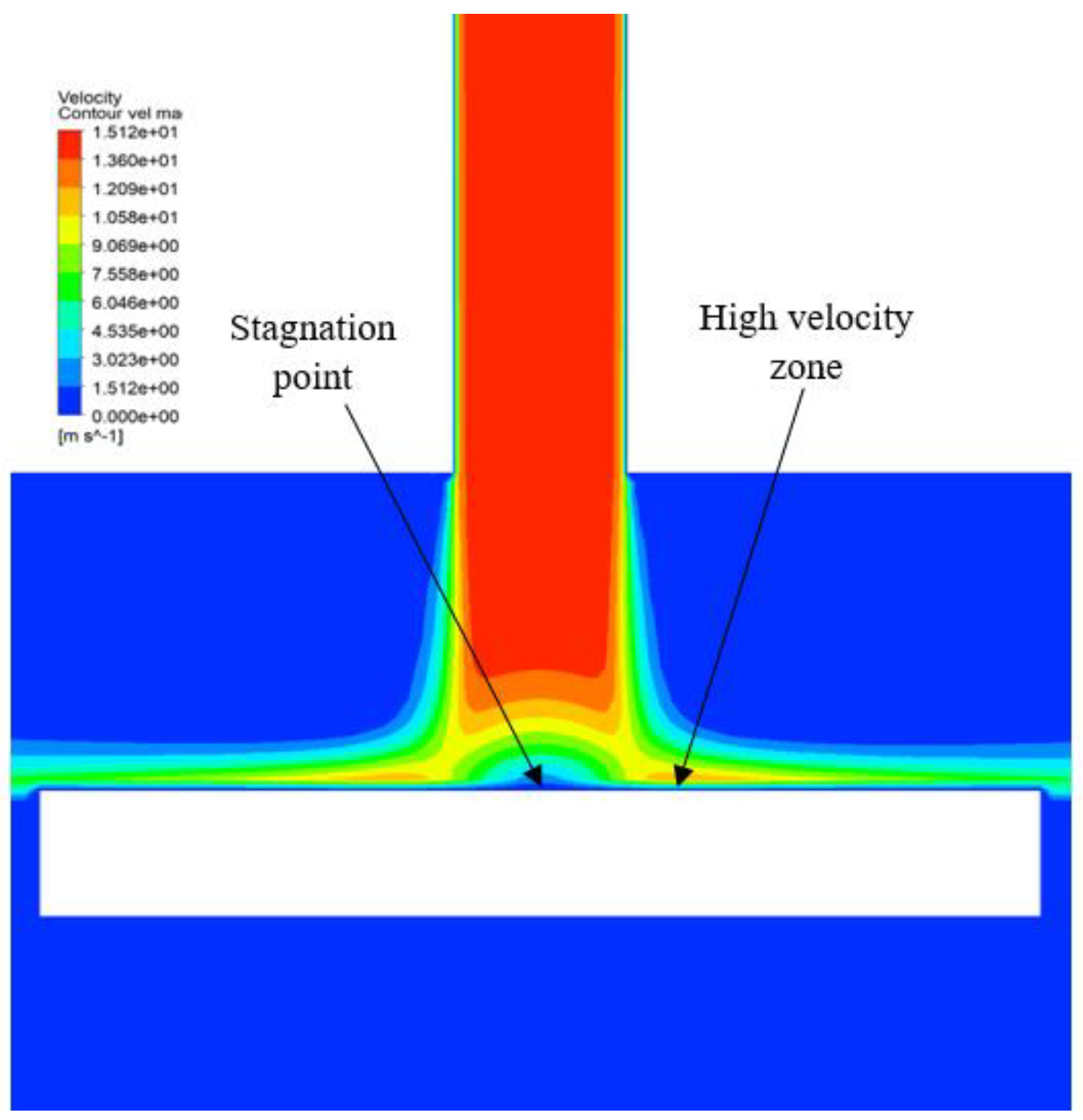
Problem Definition

The computational domain considered for the submerged jet impingement problem is shown in Figure 1. Various parameters are investigated to study the effects on solid particle erosion with water as the carrier fluid. The effects of nozzle diameter and nozzle–target distance on the erosion process are first investigated. In this part, three nozzle diameters are considered (5 mm, 7 mm, and 10 mm) at 12.7 mm nozzle–target distance, and for the 7-mm nozzle, three nozzle–target distances are considered (5 mm, 12.7 mm, and 20 mm), while keeping the circular nozzle shape, the 90° impingement angle, and the 300 µm particle sizes unchanged. The second set of simulations were focused on the effects of nozzle shape and impingement angle on the erosion process. In this part, four nozzle shapes (circular, elliptical, square, and rectangular) and three impingement angles (60°, 75°, and 90°) were considered. For the 7 mm diameter nozzle with 300 µm particle size, 90° impingement angle, and 12.7 mm clearance distance, four particle sizes (50 µm, 100 µm, 200 µm, and 300 µm) were considered.

2. Computational Modeling

The selection of the proper approach for modeling solid–fluid flow depends on the particle loading. The Eulerian–Lagrangian approach is recommended for low particle loading by volume [32], which is the case in the current study. A well-established modeling technique for the Eulerian–Lagrangian approach in estimating solid particle erosion involves sequential implementation of flow modeling, particle tracking, and erosion modeling. Numerical simulation is conducted with the commercially available CFD package, ANSYS Fluent 19.2 [32].

2.1. Flow Model

The Eulerian approach involves solving fluid flow within the computational domain by resolving the Navier–Stokes Equation. Steady-state three-dimensional mass and momentum conservation equations resolved to compute flow velocity are given as:

$$\frac{\partial u_i}{\partial x_i}=0$$

(1)

$$\frac{\partial \left(\rho u_i\right)}{\partial t}+\frac{\partial \left(\rho u_i{u}_j\right)}{\partial x_j}=-\frac{\partial p}{\partial x_i}+\frac{\partial }{\partial x_j}\left[\left(\mu +{\mu }_t\right)\left(\frac{\partial u_i}{\partial x_j}+\frac{\partial u_j}{\partial x_i}\right)\right]+\rho g_i$$

(2)

where $u$ is fluid velocity, $\rho$ is the fluid density, $p$ is the mean fluid pressure, $\mu$ is the fluid viscosity, ${\mu }_t$ is the turbulent viscosity, and $g$ is the gravitational acceleration.

A one-way particle–fluid interaction is assumed which implies only the impact of fluid on particles are accounted for; particles impact on fluid are neglected, as reflected by the inexistence of solid source term in Equation (2). Turbulence effects on the flow are modeled using the shear–stress transport (SST) k-ω model, which is a hybrid of two 2-equation models [33]. The SST k-ω turbulence model [34] is used for its capability to capture the turbulence details in the entire flow field, including the viscous sub-layer. The model is also known for its ability for predicting the flow behavior in stagnation regions and regions with strong acceleration. The Semi-Implicit Method for Pressure-Linked Equations (SIMPLE) algorithm is used to solve the pressure–velocity coupling in the equations while convective and diffusion terms are resolved with second order upwind scheme and second order central-differencing scheme, respectively.

The domain was discretized with structured mesh with refined mesh concentrated in the zone between the nozzle outlet and the target, as shown in Figure 2. Refined meshes were concentrated in the path of the jet flow and it was ensured that the first cell height from the target wall is equal to twice the particle size. This is recommended to ensure that the particles’ mean velocity and interactions between turbulent fluctuations and particles in cells adjoining the wall are adequately captured [24,25]. The grid independency test was done using four different meshes (M1 = 243,448 cells, M2 = 352,894 cells, M3 = 498,332 cells, and M4 = 750,422 cells). Figure 3 shows the velocity magnitude at 1 mm above the top of the target for the four different grids M1, M2, M3, and M4. Since the error between meshes M3 and M4 is less than μ1%, we conducted all calculation with mesh M3 (498,332 cells). The boundary conditions are shown in

Table 1. Boundary conditions for the submerged direct impact testing.

Surface/Boundary	Momentum Equation	Discrete Phase Equation
Nozzle inlet	Velocity inlet (V = Vinlet)	Escape
Nozzle wall	No slip (u = 0, v = 0, w = 0)	Escape
Target wall	No slip (u = 0, v = 0, w = 0)	Reflect
Far-away domain surface	Pressure outlet (P = 0 gage)	Escape

.

2.2. Particle Tracking

Once the fluid flow solution is achieved, the trajectories of particles are tracked and computed from the nozzle inlet to the domain outlets using the discrete phase model (DPM) by integrating the Lagrangian transport equation expressed in Equation (3) with respect to time. Turbulence effects on the particles are included and modeled using a stochastic model; the discrete random walk (DRW) model, and, to ensure the independence of erosion prediction of the number of particles, 50,000 particles are ejected at the inlet.

$$\frac{d\overrightarrow{u_p}}{dt}=\overrightarrow{F_D}+\overrightarrow{F_G}+\overrightarrow{F_{SL}}+\overrightarrow{F_{VM}}+\overrightarrow{F_P}$$

(3)

where the first term on the RHS of equation A $\overrightarrow{F_d}$is drag force per unit particle mass and is defined as the ratio of particle relative velocity $(\overrightarrow{u}-\overrightarrow{u_p)}$ to residence time ${\tau }_r$;

$$\overrightarrow{F_d}=\frac{\overrightarrow{u}-\overrightarrow{u_p}}{{\tau }_r}$$

(4)

where ${\tau }_r$ is defined in terms of particle drag coeeficient $C_d$ and particle Reynolds number $R{e}_p$ as

$${\tau }_r=\frac{24}{C_d}\frac{{\rho }_p}{18\mu }\frac{d_p^2}{R{e}_p}$$

(5)

The particle drag coefficient $C_d$, which is also a function of $R{e}_p$ and particle sphericity $\varnothing$, is an important parameter in modeling particle transport. A plot of variation of $C_d$ with respect to $R{e}_p$ and $\varnothing$ by Chochua and Shirazi [25], using the Haider and Levenspiel [35] correlation for non-spherical particles $(\varnothing$ < 1), shows that sphericity affects $C_d$ when $R{e}_p>10$ and that $C_d$ becomes lower as $\varnothing$ approaches 1 (spherical particles). $R{e}_p$ is expressed as

$$R{e}_p=\frac{\rho d_p\left|\overrightarrow{u}-\overrightarrow{u_p}\right|}{\mu }$$

(6)

The second term $\overrightarrow{F_G}$ represents buoyancy force due to gravitational acceleration and is expressed in terms of difference in densities of particle and fluid as

$$\overrightarrow{F_G}=\frac{\overrightarrow{g}\left({\rho }_p-{\rho }_f\right)}{{\rho }_p}$$

(7)

Other forces in Equation (3) that have impact on the motion of particles in fluid are Saffman lift force $\overrightarrow{F_{SL}}$, virtual mass force $\overrightarrow{F_{VM}}$, and pressure gradient force $\overrightarrow{F_p}$.

Saffman (shear) lift force is the force acting on a particle surface due to high velocity gradient, and it usually comes into play when the particle velocity is greater than the carrier fluid velocity. The virtual mass force is the force on a particle due to mass of fluid displaced by the particle while the pressure gradient force on a particle is due to fluid pressure distribution around the fluid particle. According to some studies, the virtual force and pressure gradient force are essential forces to be considered in modeling slurry erosion [25]. These forces are important when the fluid density is much larger than particle density [36]. Equation (8) shows the definition of $\overrightarrow{F_{VM}}$ and $\overrightarrow{F_p}$.

Only pressure force is included in this study as it has a more significant impact on solid particle motion in the geometry considered.

$$\overrightarrow{F_{VM}}=\frac{1}{2}\frac{{\rho }_f}{{\rho }_p}\frac{d}{dt}\left(\overrightarrow{u}-{\overrightarrow{u}}_p\right), \overrightarrow{F_p}=\frac{{\rho }_f}{{\rho }_p} {\overrightarrow{u}}_p \nabla \overrightarrow{u}$$

(8)

2.3. Erosion Model

The erosion empirical model adopted in this study is the Finnie model [37], expressed in Equation (9):

$$ER=K{V}_p^{n}f\left(\alpha \right)$$

(9)

where $ER$ is the erosion ratio (kg/kg), defined as ratio mass of material removed to mass of impinging particle, $K$ and $f\left(\alpha \right)$ are scaling parameter and impact angle function, respectively, both dependent on erodent and target material properties, $V_p$ is the particle impact velocity, and n is the exponent of particle velocity with value between 2 and 3 for ductile materials.

Table 2. Values of parameters expressed in Equations (9) and (10).

K	N	t (h)	${\mathit{\rho }}_{\mathit{w}} (\mathbf{kg}/{\mathbf{m}}^3)$
2.17 × 10−8	2.41	6	8000

shows the values of the constant parameters in the above equation. Erosion is quantified in this study in terms of thickness loss $TL$, which is depth of erosion on target material in meters.

$$TL=Erate\times t/{\rho }_w$$

(10)

where $Erate$ is the erosion rate (kg/m²-s), t is the test duration, and ${\rho }_w$ is the density of the target material, stainless steel 316.

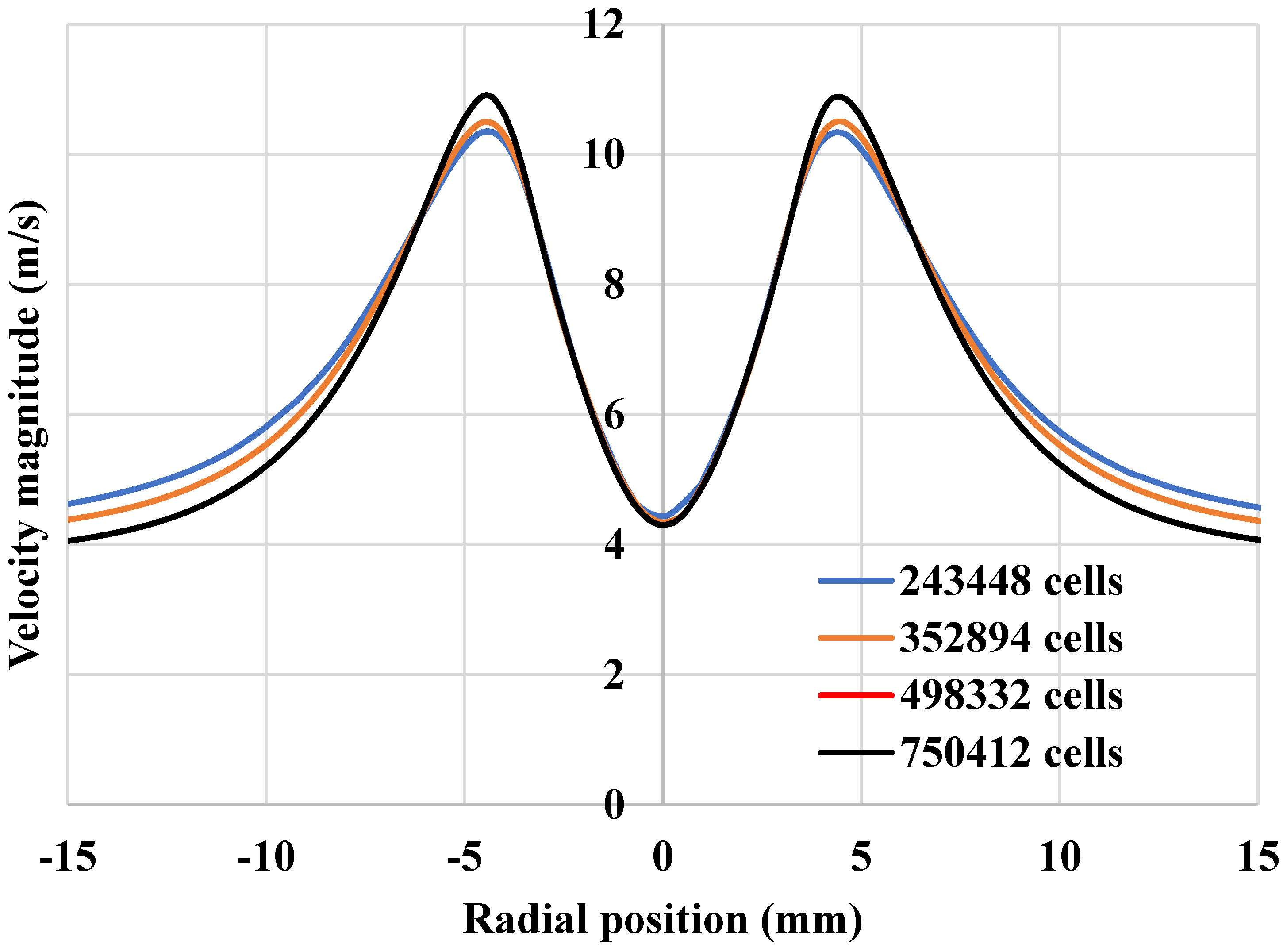
2.4. Model Validation

Figure 4 shows the comparison of erosion profiles obtained from the CFD–erosion model (with standard error bars) implemented in this work and that reported by Mansouri et al. [31] for 90° impingement angle. The case study was that of submerged direct impact erosion in water caused by 300 µm sand particles, nozzle inlet velocity of 14 m/s, and an equivalent of 1% sand concentration by mass. The locations of maximum and minimum erosion points are well-matched, while a discrepancy of 15%, on average, in the erosion depth downstream from the maximum erosion point can be observed.

3. Results and Discussion

The widely predicted erosion pattern on a wall in a submerged direct impingement setup is the W-profile, as shown in Figure 4, as well as studies reported in [20,32]. The W-erosion profile for water as carrier fluid is characterized by a zone of insignificant erosion at the center of the wall target surrounded by a highly eroded zone which is then outwardly adjoined by a low eroded zone. The equally well-known fluid characteristics of this setup can be presented as a velocity contour plot of the region between the nozzle and the wall surface, as shown in Figure 5. The fluid exiting the nozzle decelerates as it approaches the impingement point, which is the stagnation point, and afterwards is deflected radially outwards. The stagnation point corresponds to the infinitesimal erosion zone while the high-velocity region matches the highly eroded zone. Subsequently, the predicted results for the effects of geometrical and flow features on erosion characteristics of submerged jet impingement are discussed.

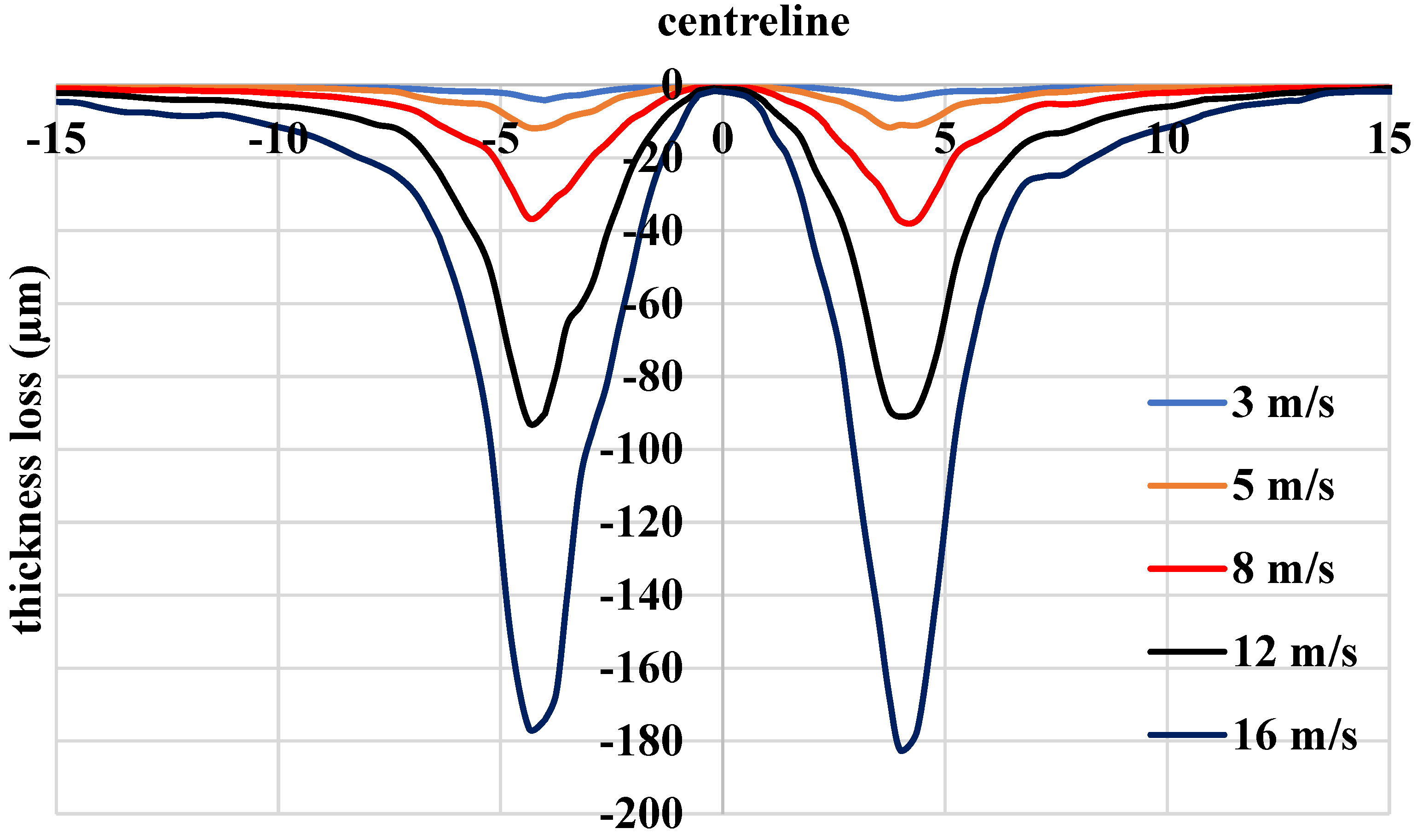
3.1. Effect of Nozzle Inlet Velocity

Unlike erosion in a straight pipe with parallel streamlines where the path of particles impacting the wall is controlled by turbulence fluctuations, the carrier fluid transports the particles directly to the wall in direct impact geometry. In addition, the trajectories of solid particles are greatly influenced by the fluid flow streamlines for low Stokes number flow, such as slurry flows [32]. Effects of inlet velocities of 3 m/s, 5 m/s, 8 m/s, 12 m/s, and 16 m/s on erosion rate for a constant circular cross-sectional nozzle outlet at 12.7 mm stand-off height from the target wall with impact angle of 90° were investigated. As shown in Figure 6, higher fluid velocity produces higher erosion rate due to higher impact velocity of the particles. The fluid velocity is directly proportional to particle impact velocity (Viera et al. [19]) and the erosion is influenced by the particle velocity according to the erosion equation. Particles conveyed by high flow velocity have high kinetic energy and momentum by virtue of high particle velocity, and erode more materials outside the stagnation region.

Momentum is a property that quantifies the magnitude of mass in motion and is directly related to the product of impact force and residence time. Since the size (mass) of the particles and carrier fluid is fixed, the time taken for the particle to respond to change in momentum (residence time) can be said to be constant. Therefore, momentum is directly proportional to impact force. Hence, increasing inlet velocity translates directly into higher impact force that causes greater target removal. It can also be seen that significant thickness loss was only observed for inlet velocities of 5 m/s and above. This aligns with the results of 5 m/s threshold velocity for significant erosion for a 90° bend pipe [38] and pipe with sudden expansion [18].

It is important to distinguish the shape of the erosion profile under a submerged water jet. As discussed by Mansouri et al. [21], there is a major difference in the erosion profile between gas–solid erosion and water–solid erosion. In the case of gas–solid erosion, the thickness loss profile has only one dip, termed as U-shape profile. In the case of the water, the erosion profile has a W shape. It has two dips away from the stagnation region.

We note that CFD simulation can reproduce this phenomenon. The difference in erosion shapes is mainly due to the difference in density ratios in both cases. In the case of air (or gas) flow, the ratio of particle density to air density is very high. In this case, the inertia of the erosive particle is much larger than that of the air. As a result, the particles do not follow the air-streamlines and do hit the central area (flow stagnation for the main phase) and produce the highest erosion rates. On the other hand, in the water case, density ratio of particle to water is about two, therefore the inertia of the water particles do affect the inertia of the particles. As a result, the stagnation region is not penetrated by the particles, and almost no erosion happens in the stagnation point of the water flow.

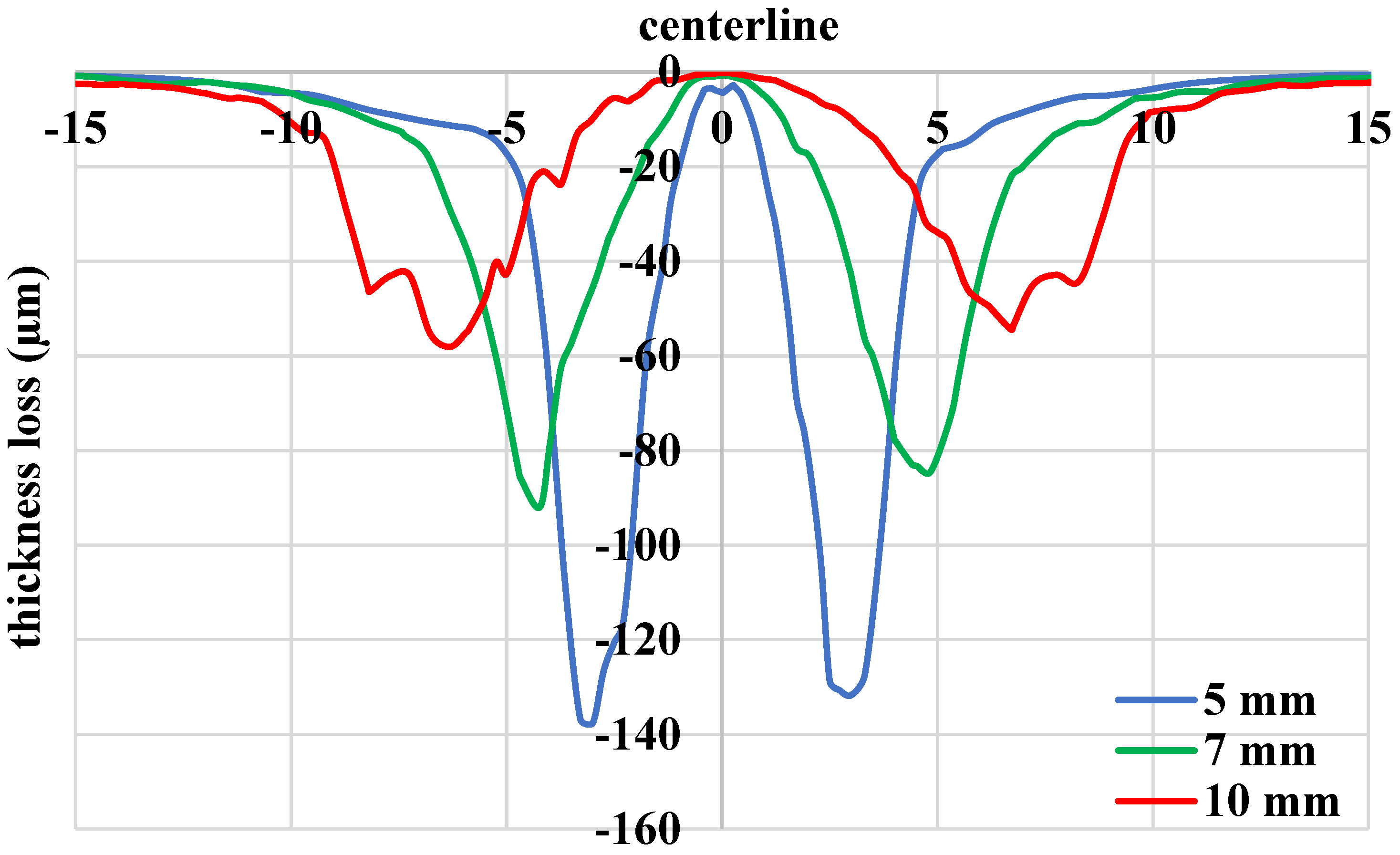
3.2. Effect of Nozzle Inlet Diameter

Figure 7 shows the plot of thickness loss profile along the centerline of the target for various circular nozzle inlet diameters of 5 mm, 7 mm, and 10 mm at constant inlet velocity of 12 m/s and atmospheric pressure. The number of particles injected was kept constant at 30,000 for all nozzle sizes considered. It is observed that the maximum thickness loss decreases with increasing nozzle diameter. This can be attributed to high impact density over a small area of the target by smaller nozzle diameter. This is also evident in the location of maximum eroded region coupled with the size of the zero-impact region at the target center. In fact, the case of the 5 mm nozzle diameter caused some material loss at the target center/stagnation zone in comparison with larger nozzle diameters.

3.3. Effect of Particle Diameter

The effect of solid particle size on erosion is presented in Figure 8. Four particle sizes of 50 µm, 100 µm, 200 µm, and 300 µm were investigated for normal impingement angle with fixed nozzle–target distance, nozzle diameter, and fluid inlet velocity of 12.7 mm, 7 mm, and 12 m/s, respectively. The location of maximum material loss increases from the target center (0) as the particle size decreases because larger particles tend to follow the path defined by the jet at the nozzle outlet due to their inertia, while smaller particles are prone to follow the fluid streamline. Thus, more smaller particles tend to strike the target material at locations of high velocity regions farther from the stagnation zone. In addition, the trend of increasing maximum material penetration depth with increasing particle size from 50 µm to 300 µm is observed, and this is due to increasing inertia force. The odd case is 100 µm particle size causing the maximum penetration depth, greater than bigger particle sizes. This can be attributed to choice of the jet impingement angle (in this case, 90°) which is closer to the maximum erosion rate angle of 100 µm than that of 300 µm, as reported by Aponte et al. [24].

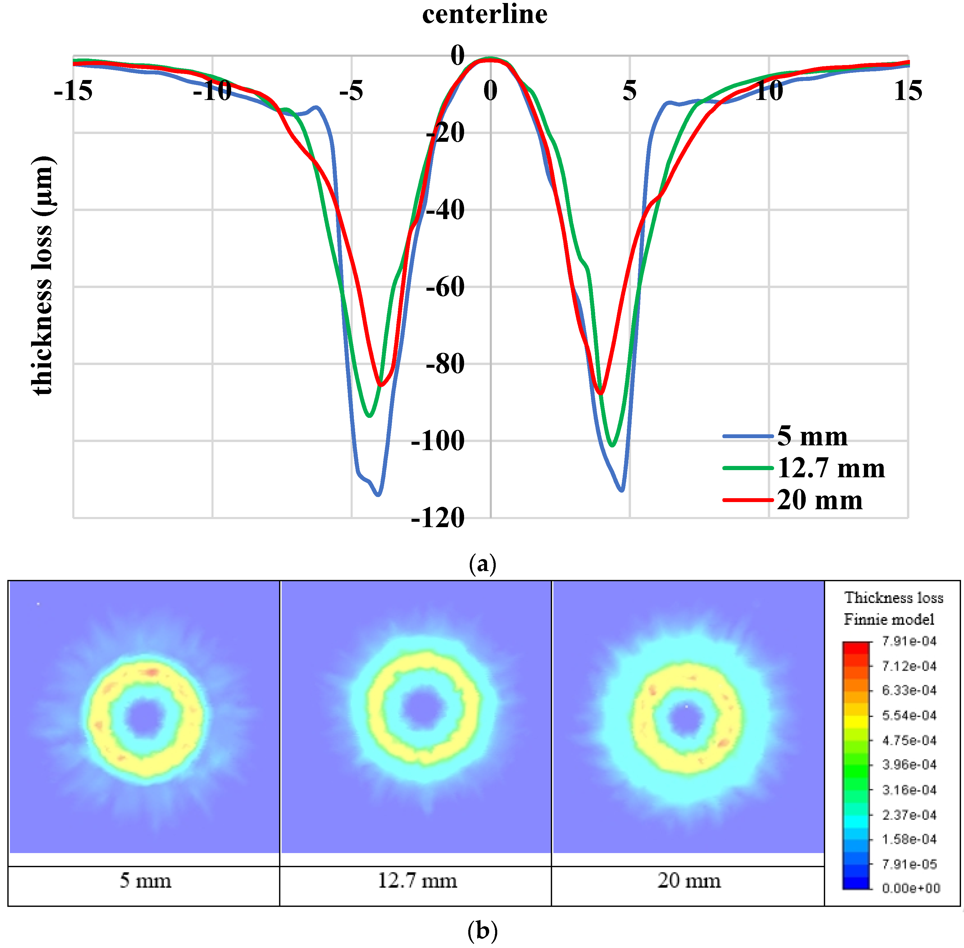
3.4. Effect of Nozzle–Target Distance/Stand-Off Height

The distance between the nozzle exit and target was varied between 5–20 mm at a constant nozzle inlet velocity of 12 m/s to study the effect of stand-off height on erosion characteristics. Figure 9a shows variation of thickness loss along the centerline on the target for the different stand-off heights considered. It is observed that the smallest nozzle stand-off height produced the highest peak thickness loss, and the peak thickness loss decreases with increasing stand-off height. This trend is due to the high number of particle impacts localized in a small region around the target center for the shortest stand-off height, causing localized high erosion, whereas the region of impact for longer stand-off height is larger, thereby leading to lower density of localized impacts and smaller peak thickness loss, as seen in contour plots drawn in Figure 9b. In addition, the region of substantial thickness loss increases with increasing separation distance.

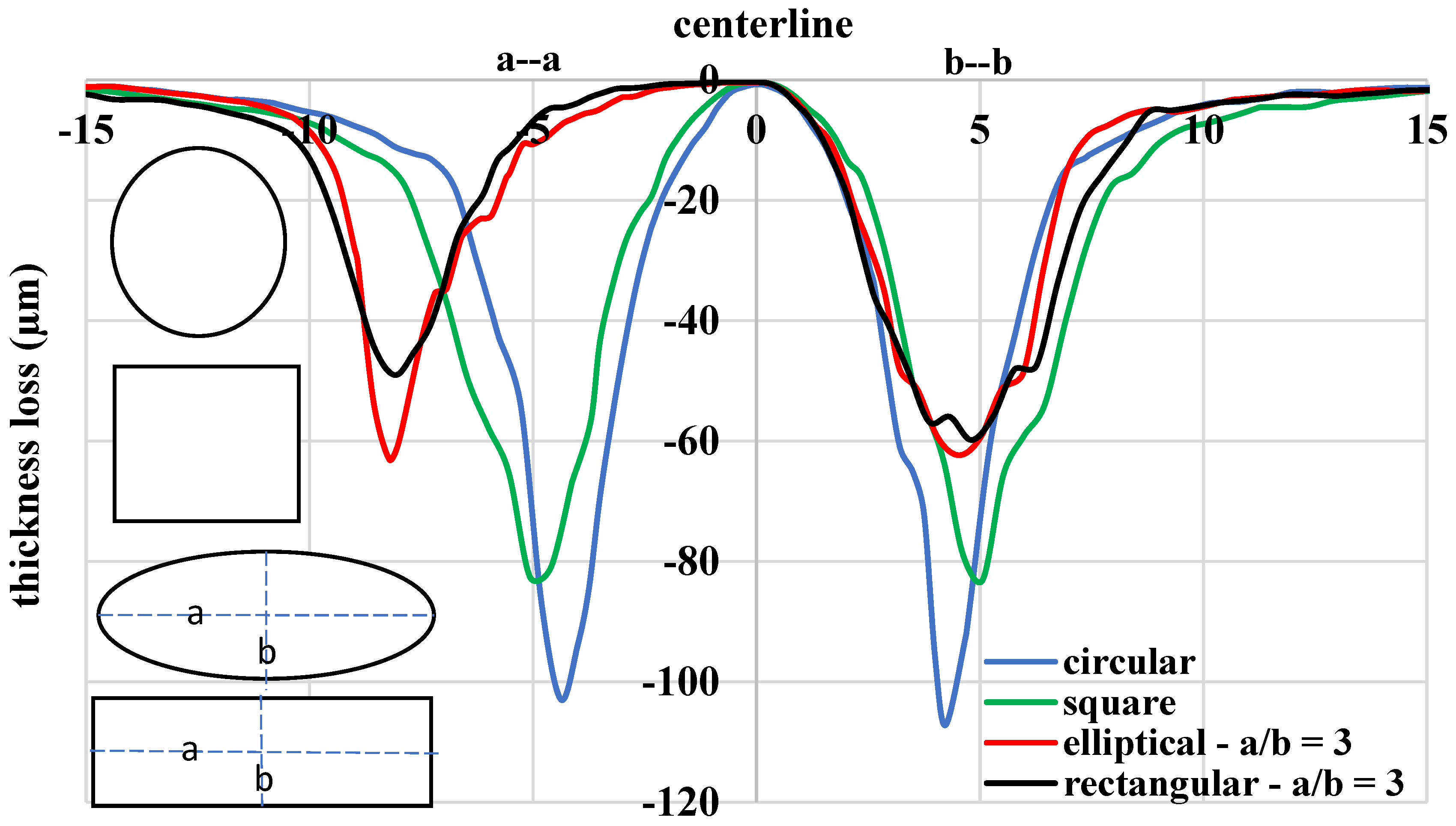
3.5. Effect of Nozzle Shape

Erosion prediction for different nozzle shapes; circular, ellipse, square, and rectangle of hydraulic diameter = 7 mm and aspect ratio a/b = 3 (for ellipse and rectangle) is shown in Figure 10. The graph consists of two plots on either side of the zero mark, each plot representing thickness loss along axes a–a and b–b on left and right sides, respectively. The particle diameter, jet impingement angle, and nozzle–jet distance are maintained at 300 µm, 90°, and 12.7 mm, respectively. It can be observed that maximum thickness loss is produced by nozzle shapes with unity aspect ratio (circle and square), with the peak loss caused by circular nozzle. Relatively symmetric thickness loss profile is observed for circular and square nozzles, while asymmetric thickness loss profiles are associated with rectangular and elliptical nozzles. This indicates that nozzle shapes influence the distribution of particles’ impact and, in effect, the pattern of eroded area of the target, especially for large particle diameters, as considered in this case. Therefore, the elliptical and rectangular nozzle produced profiles of thickness loss in one direction with wider region of zero particle impact, thereby displacing the high impact region further away from the target center.

In the above results, we can see a slight asymmetry in the erosion rates, especially in Figure 7 and Figure 8 where the effect of nozzle diameter and the effect of particle size are studied (Figure 8). We also note that the particle size of 300 micrometers gives the most asymmetry. First, note the main phase (water) flow solution gives perfectly symmetric profiles of velocity, as shown in Figure 3 and Figure 5. We can also verify this fact by the shear stress profile at the target surface symmetry line shown in Figure 11. These profiles show perfectly symmetric behavior; hence, the symmetry in the erosion rates/thickness loss profiles are due to the stochastic model used for finding the erosion rates. In this model, we tried different sampling sizes (20, 30, and 40 tries/samples per particle) until we made sure the profile was not changing anymore. It appears that this stochastic model is very sensitive to any skewness or asymmetry in the random number generation, especially for large particle diameter. We can also note there is a slight asymmetry in the experimental profiles shown in Figure 4.

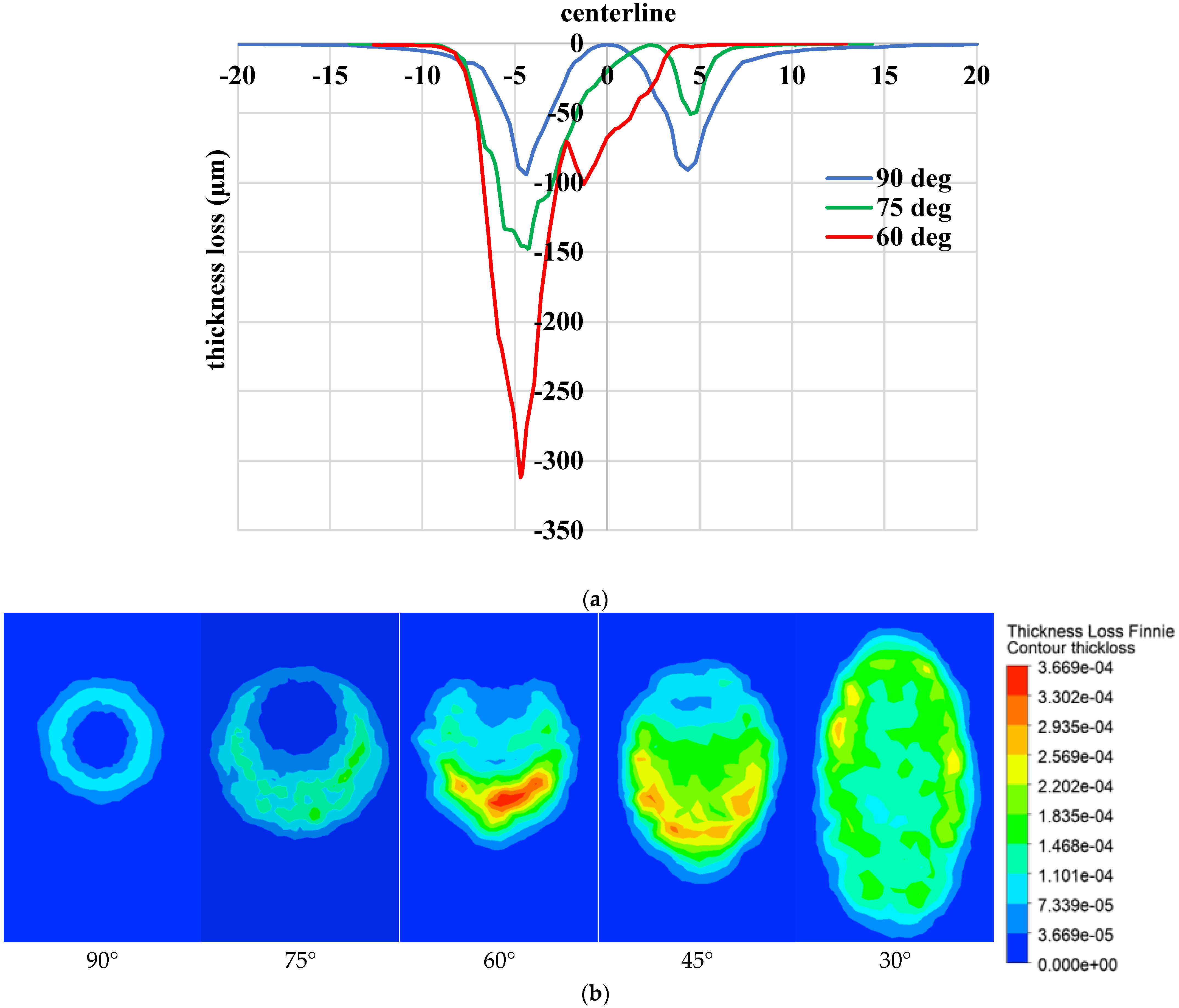
3.6. Effect of Impingement Angle

The effect of jet impingement angle on erosion behavior in a submerged direct impingement geometry with a circular cross-sectional nozzle is shown in Figure 12a. As the impingement angle decreases from 90°, the erosion profile becomes more asymmetric and the spread of the eroded area increases. This is due to the inclination angle of the target which causes a skewed concentration of particles impacting the target, thereby producing high and low impact regions on either side of the stagnation zone (zero-impact zone). Solid particle erosion tends to be higher at low impingement angles because particles are swept away by shear flow immediately after impact, thereby minimizing impact shielding by previous particles impacting the surface. As can be seen in the contour plots of thickness loss shown in Figure 12b, the 90° case caused an axisymmetric scar shape while the inclined jet cases produced a one-sided biased scar.

4. Conclusions

A numerical study of the erosion characteristics of solid–particle erosion of stainless steel 316 in a water-submerged jet impingement geometry was conducted to investigate the effects of various flow and geometric parameters, including the inlet velocity, particle size, nozzle shape and size, nozzle–target distance, and impingement angles. Erosion prediction was achieved through flow characteristics and particle tracking using the Eulerian–Lagrangian approach together with one-way coupling and erosion calculations using the Finnie model. The erosion characteristics were quantified by thickness loss profile along the target centerline and thickness loss contour plots. The accuracy of the numerical model was examined through comparisons with previously published data and a good agreement was found. On average, the difference between the experimental data and the numerical prediction is about 15%. The CFD model was capable of predicting the W-shaped erosion profile that occurs in the water which is different from the U-erosion shape that occurs in gas erosion. The results of the simulations are as follows:

• Increasing the inlet velocity leads to higher thickness loss due to increased particle impact velocity.
• The maximum thickness loss increases with increasing particle size except for 100 μm, which produced the highest. This can be attributed to closeness of the maximum erosion rate for 100 μm particle size to the choice of the jet impingement angle (in this case, 90°).
• As the nozzle size increases, the maximum thickness loss increases due to the high particle density.
• Similarly, the peak thickness loss increases slightly with increasing separation from the target.
• Finally, the erosion pattern for rectangular and elliptical nozzle is skewed.

The computational model presented in this paper need to be further developed to deal with fluids containing high percentage of solid particles (e.g., slurry flows). The model can also be developed for prediction of erosion caused by the black powder in gas pipelines in which significant damage occurs to expensive pipefittings with complicated geometry, such as valves and flowmeters.

References

- Parsi, M.; Najmi, K.; Najafifard, F.; Hassani, S.; McLaury, B.S.; Shirazi, S.A. A comprehensive review of solid particle erosion modeling for oil and gas wells and pipelines applications. J. Nat. Gas. Sci. Eng. 2014, 21, 850–873. [Google Scholar] [CrossRef]
- Flemmer, C.L.; Flemmer, R.L.C.; Means, K.; Johnson, E.K. The erosion of pipe bends. In Proceedings of the 1988 ASME Pressure Vessels and Piping Conference, Pittsburgh, PA, USA, 19–23 June 1988; pp. 93–98. [Google Scholar]
- Jafar, M.R.H.; Spelt, J.K.; Papini, M. Numerical simulation of surface roughness and erosion rate of abrasive jet micro-machined channels. Wear 2013, 303, 302–312. [Google Scholar] [CrossRef]
- Meng, H.S.; Ludema, K. Wear Models and predictive equations: Their form and content. Wear 1995, 181–183, 443–457. [Google Scholar] [CrossRef]
- Jahanmir, S. The machanics of subsurface damage in solid particle erosion. Wear 1980, 61, 309–338. [Google Scholar] [CrossRef]
- Chase, D.; Rybicki, E.; Shadley, J. A model for the effect of velocity on erosion of N80 steel tubing due to the normal impingement of solid particle. J. Energy Resour. Technol. 1992, 114, 54–56. [Google Scholar] [CrossRef]
- Salik, J.; Buckley, D.; Brainard, W. The effect of mechanical surface and heat treatments on erosion resistance of 6061 aluminum alloy. Wear 1981, 65, 351–358. [Google Scholar] [CrossRef]
- Levy, A.; Chik, P. The effect of erodent composition and shape on the erosion of steel. Wear 1983, 89, 151–162. [Google Scholar] [CrossRef]
- Barton, P.T.; Drikakis, D.; Romenski, E.I. An Eulerian finite-volume scheme for large elastoplastic deformations in solids. Int. J. Numer. Methods Eng. 2010, 81, 453–484. [Google Scholar] [CrossRef]
- Barton, P.T.; Drikakis, D. An Eulerian method for multi-component problems in non-linear elasticity with sliding interfaces. J. Comput. Phys. 2010, 229, 5518–5540. [Google Scholar] [CrossRef]
- Barton, P.T.; Obadia, B.; Drikakis, D. A conservative level-set based method for compressible solid/fluid problems on fixed grids. J. Comput. Phys. 2011, 230, 7867–7890. [Google Scholar] [CrossRef]
- Clark, H.M. On the impact rate and impact energy of particles in a slurry pot erosion tester. Wear 1991, 146, 165–183. [Google Scholar] [CrossRef]
- Sundararajan, G. A comprehensive model for the solid particle erosion of ductile materials. Wear 1991, 149, 111–127. [Google Scholar] [CrossRef]
- Arabnejad, H.; Shirazi, S.A.; McLaury, B.S.; Subramani, H.J.; Rhyne, L.D. The effect of erodent particle hardness on the erosion of stainless steel. Wear 2015, 332–333, 1098–1103. [Google Scholar] [CrossRef]
- Badr, H.M.; Habib, M.A.; Ben-Mansour, R.; Said, S.A.M.; Al-Anizi, S.S. Erosion in the tube entrance region of an air-cooled heat exchanger. Int. J. Impact Eng. 2006, 32, 1440–1463. [Google Scholar] [CrossRef]
- Habib, M.A.; Ben-Mansour, R.; Badr, H.M.; Said, S.A.M.; Al-Anizi, S.S. Erosion in the tube entrance region of a shell and tube heat exchanger. Int. J. Numer. Methods Heat Fluid Flow 2005, 15, 143–160. [Google Scholar] [CrossRef]
- Badr, H.M.; Habib, M.A.; Ben-Mansour, R.; Said, S.A.M. Numerical investigation of erosion threshold velocity in a pipe with sudden contraction. Comput. Fluids 2005, 34, 721–742. [Google Scholar] [CrossRef]
- Habib, M.A.; Badr, H.M.; Ben-Mansour, R.; Kabir, M.E. Erosion rate correlations of a pipe protruded in an abrupt pipe contraction. Int. J. Impact Eng. 2007, 34, 1350–1369. [Google Scholar] [CrossRef]
- Vieira, R.E.; Mansouri, A.; McLaury, B.S.; Shirazi, S.A. Experimental and computational study of erosion in elbows due to sand particles in air flow. Powder Technol. 2016, 288, 339–353. [Google Scholar] [CrossRef]
- Messa, G.V.; Malavasi, S. The effect of sub-models and parameterizations in the simulation of abrasive jet impingement tests. Wear 2017, 370–371, 59–72. [Google Scholar] [CrossRef]
- Liu, Z.G.; Wan, S.; Nguyen, V.B.; Zhang, Y.W. A numerical study on the effect of particle shape on the erosion of ductile materials. Wear 2014, 313, 135–142. [Google Scholar] [CrossRef]
- Messa, G.V.; Malavasi, S. A CFD-based method for slurry erosion prediction. Wear 2018, 398–399, 127–145. [Google Scholar] [CrossRef]
- Parsi, M.; Jatale, A.; Agrawal, M.; Sharma, P. Effect of surface deformation on erosion prediction. Wear 2019, 430–431, 57–66. [Google Scholar] [CrossRef]
- Aponte, R.D.; Teran, L.A.; Ladino, J.A.; Larrahondo, F.; Coronado, J.J.; Rodríguez, S.A. Computational study of the particle size effect on a jet erosion wear device. Wear 2017, 374–375, 97–103. [Google Scholar] [CrossRef]
- Chochua, G.G.; Shirazi, S.A. A combined CFD-experimental study of erosion wear life prediction for non-Newtonian viscous slurries. Wear 2019, 426–427, 481–490. [Google Scholar] [CrossRef]
- Karimi, S.; Shirazi, S.A.; McLaury, B.S. Predicting fine particle erosion utilizing computational fluid dynamics. Wear 2017, 376–377, 1130–1137. [Google Scholar] [CrossRef]
- Frosell, T.; Fripp, M.; Gutmark, E. Investigation of slurry concentration effects on solid particle erosion rate for an impinging jet. Wear 2015, 342–343, 33–43. [Google Scholar] [CrossRef]
- Zhang, Y.; Reuterfors, E.P.; McLaury, B.S.; Shirazi, S.A.; Rybicki, E.F. Comparison of computed and measured particle velocities and erosion in water and airflows. Wear 2007, 263, 330–338. [Google Scholar] [CrossRef]
- Mansouri, A. Development of Erosion Equations for Slurry Flows; Erosion/Corrosion Research Center: Tulsa, OK, USA, 2014. [Google Scholar]
- Parsi, M.; Kara, M.; Sharma, P.; McLaury, B.S.; Shirazi, S.A. Comparative study of different erosion model predictions for single-phase and multiphase flow conditions. In Proceedings of the Offshore Technology Conference, Houston, TX, USA, 2–5 May 2016; Volume 5, pp. 3926–3945. [Google Scholar] [CrossRef]
- Mansouri, A.; Arabnejad, H.; Shirazi, S.A.; McLaury, B.S. A combined CFD/experimental methodology for erosion prediction. Wear 2014, 332–333, 1090–1097. [Google Scholar] [CrossRef]
- ANSYS Inc. Ansys Fluent Theory Guide. In Ansys® Academic Research Mechanical; ANSYS Inc.: Canonsburg, PA, USA, 2018; Release 19.2. [Google Scholar]
- Menter, F.R. 2-Equation eddy-viscosity turbulence models for engineering applications. AIAA J. 1994, 32, 1598–1605. [Google Scholar] [CrossRef]
- Menter, F.R. Zonal Two Equation k-ω Turbulence Models for Aerodynamic Flows. In Proceedings of the AIAA Paper, Orlando, FL, USA, 6–9 July 1993; pp. 93–2906. [Google Scholar]
- Haider, A.; Levenspiel, O. Drag coefficient and terminal velocity of spherical and nonspherical particles. Powder Technol. 1989, 58, 63–70. [Google Scholar] [CrossRef]
- Darihaki, F.; Hajidavalloo, E.; Ghasemzadeh, A.; Safian, G.A. Erosion prediction for slurry flow in choke geometry. Wear 2017, 372–373, 42–53. [Google Scholar] [CrossRef]
- Finnie, I. Erosion of Surfaces by Solid Particles. Wear 1960, 3, 87–103. [Google Scholar] [CrossRef]
- Safaei, M.R.; Mahian, O.; Garoosi, F.; Hooman, K.; Karimipour, A.; Kazi, S.N.; Gharehkhani, S. Investigation of micro- and nanosized particle erosion in a 90° pipe bend using a two-phase discrete phase model. Sci. World J. 2014, 2014, 1–12. [Google Scholar] [CrossRef] [PubMed]