Article

Analysis of Small Hydropower Generation Potential: (1) Estimation of the Potential in Ungaged Basins

1
Division of Computer Science and Engineering, Sahmyook University, Seoul 01795, Korea
2
Department of Civil Engineering, Inha University, Incheon 22212, Korea
3
Construction Technology Safety Department, Korea Institute of Civil Engineering and Building Technology, Ilsan 10223, Korea
4
Institute of Water Resources System, Inha University, Incheon 22212, Korea
*
Author to whom correspondence should be addressed.
Energies 2021, 14(11), 2977; https://doi.org/10.3390/en14112977
Submission received: 16 October 2020 / Revised: 18 January 2021 / Accepted: 11 February 2021 / Published: 21 May 2021
(This article belongs to the Section A3: Wind, Wave and Tidal Energy)

Abstract

:
Small hydropower (SHP) plants are advantageous as they have a short construction period and can be easily maintained. They also have a higher energy density than other alternative energy sources as environmentally-friendly energy sources. In general, hydropower potential is estimated based on the discharge in the river basin, and the discharge can be obtained from the stage station in the gaged basin. However, if there is no station (i.e., ungaged basin) or no sufficient discharge data, the discharge should be estimated based on rainfall data. The flow duration characteristic model is the most widely used method for the estimation of mean annual discharge because of its simplicity and it consists of rainfall, basin area, and runoff coefficient. Due to the characteristics of hydroelectric power depending on the discharge, there is a limit to guaranteeing the accuracy of estimating the generated power with only one method of the flow duration characteristic model. Therefore, this study assumes the gaged basins of the three hydropower plants of Deoksong, Hanseok, and Socheon in Korea exist as ungaged basins and the river discharges were simulated using the Kajiyama formula, modified-TPM(Two-Parameter Monthly) model, and Tank model for a comparison with the flow duration characteristics model. Furthermore, to minimize the uncertainty of the simulated discharge, four blending techniques of simple average method, MMSE(Multi-Model Super Ensemble), SMA(Simple Model Average), and MSE(Mean Square Error) were applied. As for the results, the obtained discharges from the four models were compared with the observed discharge and we noted that the discharges by the Kajiyama formula and modified-TPM model were better fitted with the observations than the discharge by the flow duration characteristics model. However, the result by the Tank model was not well fitted with the observation. Additionally, when we investigated the four blending techniques, we concluded that the MSE technique was the most appropriate for the discharge simulation of the ungaged basin. This study proposed a methodology to estimate power generation potential more accurately by applying discharge simulation models that have not been previously applied to the estimation of SHP potential and blending techniques were also used to minimize the uncertainty of the simulated discharge. The methodology proposed in this study is expected to be applicable for the estimation of SHP potential in ungaged basins.

1. Introduction

Hydropower is a clean regenerative energy source that is fueled by water and sustainable even in future climate change scenarios [1]. It contributes to the reduction of carbon emissions [2], and produces electricity from generators connected to water turbines while increasing the rotational power of the water turbines using a head. It is considered as a resource that has a high development value because it has a higher energy density than other alternative energy sources. Hydropower generation has been undervalued because of its high initial installation cost; however, because of the environmental concerns regarding the carbon emissions from fossil fuel burning and radioactive hazards from nuclear power plants, hydropower generation, especially small hydropower (SHP), which enables local distributed energy generation, is being re-examined as a clean energy source. Hydropower is classified based on the power capacity. According to the classification criteria, a hydropower plant generating the capacity of 10,000 kW or less is defined as SHP [3].
The SHP potential is the sum of small hydropower resources corresponding to the annual maximum power generation [4]. Since it is determined by water quantity and terrain conditions, discharge is the core parameter for estimating the SHP potential [5]. There are SHP plants with 208 MW facilities installed at 251 locations in Korea. They produce 545 GWh/year, and have an average facility capacity of 1617 kW. The facility capacity and power generation of the theoretical hydropower generation potential presented in the ‘New and renewable energy white paper in 2018′ have been calculated as 28 GW and 246 TWh/year, respectively, and the technological potential are calculated as 12 GW and 41 TWh/year, respectively [6].
Adhau et al. (2012) calculated the power generation potential and the capacity of SHP plants using hydropower time series data for the last six decades to locate feasible sites for SHP generation in India [7]. Larentis et al. (2010) calculated the discharge values and used them as input data for a potential estimation module in an equation to calculate the potential of hydropower plant candidate sites [8,9]. Many studies have measured the discharge over a long period to determine the available discharge at hydropower generation sites [9,10,11,12,13,14,15,16]. Noyes (1980) and Park and Lee (2008) simulated the discharge by analyzing rainfall data measured at nearby stations when the discharge and stage stations were insufficient for discharge simulations [17,18]. Yu et al. (2017) calculated the annual mean discharge, plant capacity, and annual SHP generation by unit head to analyze the potential resources [9]. Gossain and Rio (2005), Kusre et al. (2009), and Thin et al. (2020) estimated hydropower potential using the GIS(Geographic Information System) and SWAT(Soil & Water Assessment Tool) model [19,20,21]. As shown in these examples, many studies have estimated the SHP potential using the discharge data based on the rainfall data [10,13,14,18,19,20,21,22]. Previous studies suggest using measured discharge data when there are a sufficient amount of data and estimating discharge using the precipitation data from rainfall stations when the measured discharge data are insufficient or unavailable [4].
Thus, in gaged basins, to measure the discharge data that can be used to calculate the SHP potential, but in ungaged basins with no measured discharge data, discharge should be calculated to estimate the SHP potential. To accurately calculate discharge, the flow-duration characteristics model of Park and Lee (2008) is typically applied using rainfall data. This method estimates the hydropower potential of a site by calculating the annual mean discharge using annual precipitation data, basin area, and runoff coefficient [13,18]. Cheng et al. (2017) simulated the monthly potential of an SHP plant in an ungaged basin using the Grey model [23]; Zlatanović et al. (2014) calculated the discharge values in an ungaged basin using an open source software application [24]; and Saliha et al. (2011) estimated the discharge values in an ungaged basin by combining a hydrological model and neural network theory [25].
Kim et al. (2018) estimated the SHP potential by using a grid-based surface runoff model [26]. Kim et al. (2012) calculated the discharge data by applying the Tank model while investigating the variations in SHP generation due to climate change [27]. Other studies have predicted future SHP generation potential through runoff simulations by using hydrological models [28,29,30,31,32,33]. However, to improve the accuracy of the power generation potential, the reliability of the models should be verified by comparing the results of various methods with the potential estimated using conventional methods. For this purpose, monthly data should be derived using runoff models to calculate the parameters such as seasonal discharge variations, plant capacity, and the efficiency of power plants for the estimation of power generation potential.
The goal of this research was to improve the reliability of the power generation potential predictions in an ungaged basin. The discharge data are calculated using several runoff formulas and hydrologic models rather than only using a simple flow-duration characteristics model [34,35,36]. Specifically, the discharge was estimated using the empirical Kajiyama formula, the modified-TPM (two-parameter monthly) water balance model [37], which calculates the runoff using hydrologic/weather data, and the Tank model, which calculates the discharge based on the rainfall–runoff processes. The uncertainties of the models were minimized by applying four ensemble blending techniques (simple average method, multi-model super ensemble (MMSE), simple multi-model average (SMA), and mean square error (MSE) to the calculated discharge values. In Section 2, methodologies for simulating runoff and blending of runoff results are presented, and in Section 3, the runoff results are simulated through each method by applying them to three small hydro power plants and blending through each technique. Each of the results was compared and analyzed. Finally, Section 4 presents the discussion and conclusions of this study.

2. Methodology

2.1. Rainfall–Runoff Analysis

2.1.1. Flow-Duration Characteristics Model

Existing studies on hydropower generation potential have calculated the discharge data using the flow-duration characteristics model proposed by Park and Lee (2008) with precipitation data, runoff coefficient, and basin area used as input [18]. This method converts the observed precipitation data into discharge to estimate the SHP potential. Given that the runoff coefficient ( C ) stays constant throughout the year, the annual mean discharge ( Q , m 3 / s ) in a river can be calculated from the annual precipitation ( R , mm) and basin area ( A , km 2 ) using the following equation:
Q   =   R   ×   10 3   ×   A   ×   10 6   ×   C 365   ×   24 ×   60   ×   60

2.1.2. Kajiyama Formula

The Kajiyama formula, which was published by Kajiyama in Japan in 1929, is an empirical formula used to calculate the water storage capacity of a hydropower plant and estimate the flow rate at locations with no runoff data. The Kajiyama formula is used to calculate the runoff depth by using monthly precipitation data as input for deriving the rainfall–runoff relationship [38].
q = P 2   +   ( 138.6 f + 10.2 ) 2 138.6 f + E ,
where q is the monthly runoff depth (mm); P is the monthly precipitation (mm); f is the runoff coefficient (mm); and E is the monthly correction discharge (mm).
The Kajiyama formula is convenient for most locations because it only uses monthly precipitation as input data, but its theoretical basis is weak and it causes problems when applied to different basins as it applies the same E value to each basin without considering the differences in river characteristics.

2.1.3. Modified-Two-Parameter Monthly (TPM) Water Balance Model

Modified-TPM proposed by Kim et al. (2016) is a modified version of the two-parameter monthly water balance model (TPM) proposed by Xiong and Guo (1999) [37,39] and presents a methodology for estimating two model parameters S (soil moisture content) and SC (field capacity) in TPM. TPM analyzes the relationship of these model parameters with meteorological and topographic factors. Model parameter c, which is related to evapotranspiration, is used to change the temporal scale from an annual to monthly scale. The discharge is measured based on the relationship between the actual and potential evapotranspiration suggested by Penman. Model parameter SC (field capacity) represents the amount of water that remains in the soil after excess gravitational water infiltrates into the ground. SC is related to the mean curve number (CN) of the AMC-II (Antecedent Soil Moisture Condition II) based on the soil type, land use, and treatment conditions in a basin.
To build a model, the actual evapotranspiration should be calculated using the potential evaporation obtained from the measurements. The actual annual evapotranspiration can be calculated using the following equations proposed by Brutsaert (1992) [40]:
E ( t )   =   EP ( t ) × tan h [ P ( t ) EP ( T ) ]  
where E ( t ) is the actual annual evapotranspiration (mm); EP ( t ) is the potential annual evapotranspiration (mm); and P ( t ) is the annual precipitation (mm).
After conducting many numerical experiments, Xiong and Guo (1999) [39] presented Equation (4) to calculate the actual monthly evapotranspiration from the monthly evapotranspiration by multiplying Equation (3) by coefficient c.
E ( t )   =   c × EP ( t ) × tan h [ P ( t ) EP ( T ) ]
The relationship between runoff depth q ( t ) and S in the model is a hyperbolic tangent relationship as expressed in Equation (5).
q ( t )   =   S ( t ) × tan h [ S ( t ) / SC ]
where q ( t ) is the monthly runoff depth (mm); S ( t ) is the soil moisture content (mm); and SC is the field capacity (mm). Monthly runoff Q ( t ) is related to soil moisture content S [39].

2.1.4. Tank Model

The Tank model is a lumped concept model developed by Sugawara in 1961 in Japan to conduct runoff analysis by assuming the study basin as a vertically aligned tank, similar to modeling a groundwater structure [41]. This can be practically applied even when the measurement data are insufficient or when the basin is ungaged because the model structure is relatively simple and the number of input data and parameters required for runoff analysis is small.
In the Tank model, each tank has one or more outlets at the bottom and on the sides. The outlet on the sides represents the initial and intermediate runoff, and the outlet at the bottom represents infiltration and percolation. The side outlet of the first tank represents surface water runoff, which infiltrates to the second tank through the bottom outlet. The side outlet of the second tank signifies the intermediate runoff and percolates to the lower tank and becomes groundwater runoff [42].

2.2. Blending Techniques

Even with the same rainfall events, the results can be different if runoff analysis is conducted by applying different hydrological models, decreasing the accuracy of the hydrological model. In this case, the model is generally corrected by using one rainfall–runoff model with various parameter sets. However, this creates the problem of ignoring the systematic uncertainty of the model. To solve this problem, blending techniques have been proposed [43]. Blending techniques reduce the uncertainty of the model by combining multiple models to obtain an improved simulation result and increase the usability of the model [44,45]. Many blending techniques using simple or weighted means, multiple linear regression analysis, and Bayesian model have been suggested. The blending techniques used in this study are introduced below.

2.2.1. Multi-Model Super Ensemble (MMSE)

The multi-model super ensemble (MMSE) technique is a multiple model simulation approach widely used in weather simulations. The MMSE technique is expressed as follows [46]:
( Q MMSE ) t   =   Q obs ¯   +   i = 1 N x i   ( ( Q s   im ) i ,   t     ( Q s   im ¯ ) i ) ,
where ( Q MMSE ) t is the multiple model prediction obtained through the MMSE Equation at time t ; ( Q s   im ) i ,   t is the runoff value of the ith model at time t ; ( Q s   im ¯ ) i is the mean of the ith model discharge values over the entire period; Q obs ¯ is the mean of the measured values; and x i (where i = 1 , 2 , , N ) is the regression coefficient of each of the N models, which can be determined through regression analysis.

2.2.2. Simple Model Average (SMA)

Simple model average (SMA) is a multiple model ensemble technique proposed by Georgakaos (2004) [43]. It evaluates the ensemble runoff simulations by calculating the average result of each model and compares the runoff and average values of the models at each time point. The SMA technique is expressed as follows:
( Q SMA ) t   =   Q obs ¯   +   i = 1 N ( Q s   im ) i ,   t ( Q s   im ¯ ) i N
where ( Q SMA ) t is the multiple model simulation value obtained through the SMA Equation at time t ; Q obs ¯ is the average of the measured values during the measurement period; ( Q s   im ) i ,   t is the discharge value of the ith model at time t ; and ( Q s   im ¯ ) i is the average of the discharge values of the ith model over the entire period.

2.2.3. Mean Square Error (MSE)

The mean square error (MSE) technique determines the mean square error using the simulated discharge and mean square error of each model and presents one integrated runoff curve from the runoff curves of multiple models. In other words, it determines one integrated runoff curve by combining multiple models using the weight obtained based on the performance of one model through the calibration of a single model. The MSE technique is expressed as follows:
MSE i   =   t = 1 T ( Q t i     Q SM t i ) 2
W i   =   MSE i   1 i = 1 N MSE i   1
Q MM Q t   =   i = 1 N Q SM t i   ×   W i
where W i = 0~1; Q t i is the measured discharge at time t; and Q SM t i is the discharge value of the ith model at time t, which are used to determine the MSE of the ith model. Since a lower MSE results in a higher model accuracy, the reciprocal of the MSE value was taken and a higher weight was assigned to a model that had a higher performance capacity as in Equation (9). One integrated multiple model simulation value can be determined as in Equation (10) by summing the simulated discharge of each model multiplied by the weight obtained using Equation (9).

2.3. Calculation of Small Hydropower (SHP) Potential

Hydropower is the total energy of water precipitated on the surface of a basin, and the total energy is the theoretical potential. The theoretical potential minus the loss due to runoff according to the geographic characteristics is called the geographic potential, and the water energy that can be utilized considering the system efficiency and utilization rate corresponds to the technical potential.
If the water quantity used by the water turbine per unit time is Q ( m 3 / s ), the head is H (m), the water density is ρ (kg/m3), and the theoretical potential is P t =   ρ ·g·Q·H ( kW ). If the efficiency of the water turbine generator (efficiency of the device and the ratio of the output to the input) is η, the technical potential becomes P =   ρ ·g· Q d · H e · η ( kW ). The g is gravity acceleration ( m / s 2 ) , and Q d ( m 3 / s ) and H e   ( m ) indicate the design discharge and effective head respectively. The effective head ( H e ) means the head of height, which contributes to the energy. It can be obtained by excluding loss head (head loss) from the gross head. The total efficiency (η) of the water turbine generator varies by the size and type of the device. The smaller the capacity, the lower the total efficiency. The total efficiency of water turbines and generators in power plants is 0.84–0.92.
To calculate the potential SHP energy of a target basin, the discharge data measured at a hydrological station in the target basin are used. However, there are many ungaged basins because discharge stations are installed only in some basins, and there are not many stations that provide usable data. In such ungaged basins, the discharge is simulated using flood tracking technology and long-term discharge data. However, if this method is not feasible because of the time requirement and high cost, a specific discharge method can be used to apply the runoff rate of each standard basin and evaluate the relevance of the runoff relative to the river size by flood tracking in river master plans [42].

3. Runoff Simulation and Small Hydropower (SHP) Potential in Ungaged Basins

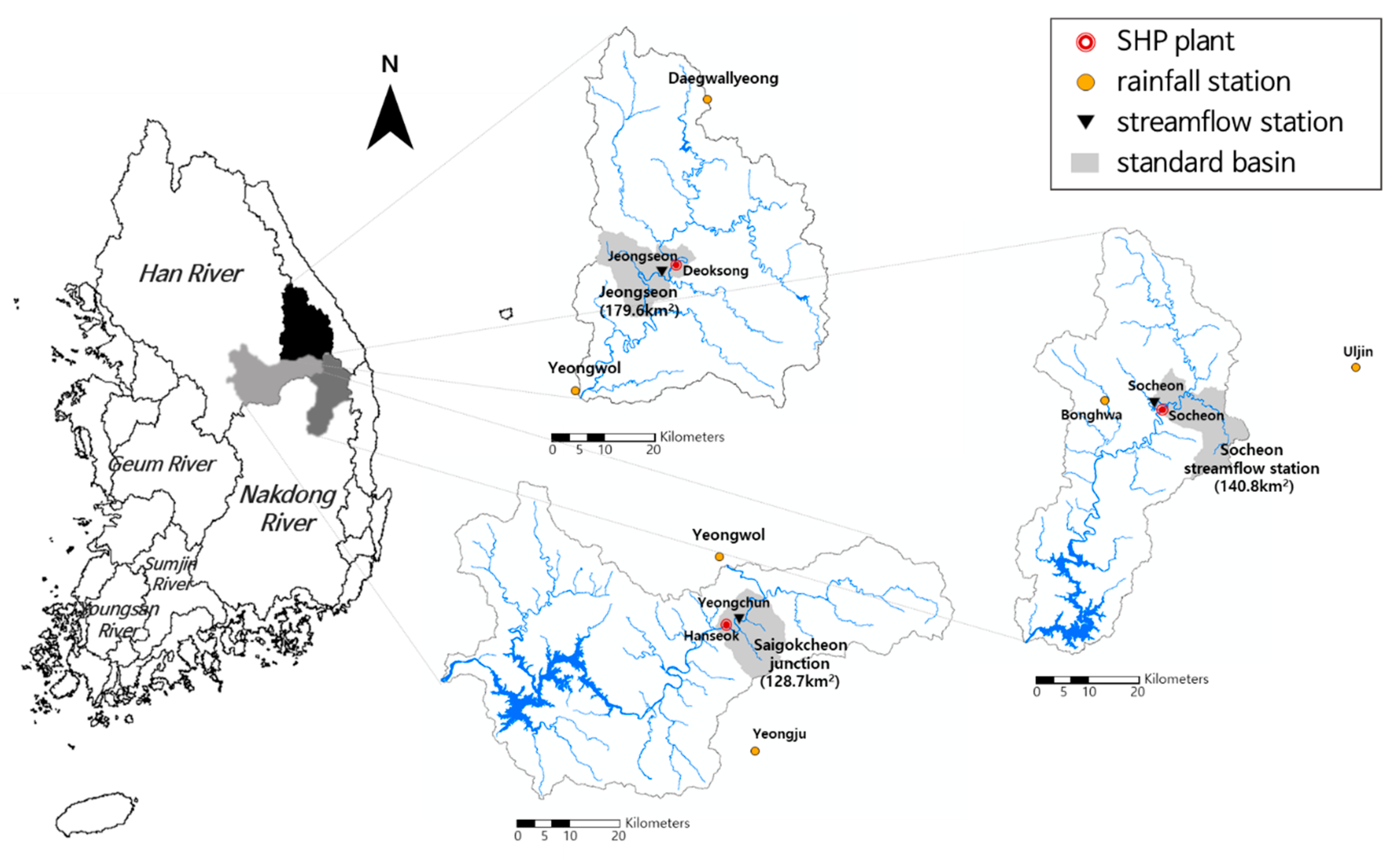
3.1. Target Basin and Data Collection

3.1.1. Target Basin

To derive a method to calculate runoff and SHP potential in ungaged basins, gaged basins were selected as target basins and the runoff and potential were calculated using the proposed methodology. Then, the methodology was verified by comparing the calculated results with the measured values. In this study, out of 61 SHP plants (as of 2015) currently in operation, the Deoksong Power Plant (in Jeongseon-gun, Korea) and the Hanseok Power Plant (in Danyang-gun, Korea) in the Han River basin, and the Socheon Power Plant (in Bonghwa-gun, Korea) in the Nakdong River basin were selected. The selection criteria included the existence of a rainfall station with available weather data and the existence of a stage station to verify the calculated discharge in the standard basin where a SHP plant exists. Other criteria included the existence of over 2000 kW of the power plant capacity, private power plants that guarantee stable power plant operation, and the possession of power generation data for 10 years or longer.
The runoff simulation to calculate the power generation potential of the target SHP plant was performed for each standard basin in which a power plant is located. The Deoksong SHP plant with a capacity of 2600 kW has been generating electricity since its construction in 1993. It is located in the Jeongseon standard basin, and Yeongwol and Daegwallyeong rainfall stations are in operation under the Korea Meteorological Administration (KMA) near the plant. The discharge data from the Jeongseon stage station were used. The Hanseok SHP plant with a capacity of 2214 kW has been generating electricity since its construction in 1989. It is located in the standard basin of the Saigokcheon junction, and Yeongwol and Yeongju rainfall stations are in operation under the KMA near the plant. The discharge data from the Yeongchun stage station were used in the simulation. The Socheon SHP plant with a capacity of 2400 kW has been generating electricity since its construction in 1987. It is located in the Socheon streamflow station standard basin, and Uljin and Bonghwa rainfall stations are in operation under the KMA near the plant. The discharge data from the Socheon stage station were used in the analysis.
The effective head, generation flow rate, generation capacity, and other information on the three selected SHP plants are summarized in Table 1. The general characteristics of each standard basin and the specifications of nearby stations are outlined in Table 2, Table 3 and Table 4. The location of target basins, SHP plants and stations is shown in Figure 1.

3.1.2. Collection and Analysis of Hydrological and Meteorological Data

To calculate runoff, monthly and daily precipitation data from five weather measurement points (Daegwallyeong, Yeongwol, Uljin, Bonghwa, and Yeongju) that influence the standard basins where the Deoksong, Hanseok, and Socheon SHP plants are located were collected first. The data for 10 years from January 2008 to December 2017 were used along with the available discharge data. The Penman method was used to calculate the potential evapotranspiration when applying the TPM method for runoff analysis. The monthly mean data for temperature (88 °C), relative humidity (%), and wind speed (m/s) were also collected for the same period at each measurement point.
When applying the weather data at each point for discharge analysis of the basins, the average values over the area representing each basin should be calculated. The Thiessen polygon method was applied to calculate the areal precipitation, which is frequently used in practice. The average areal precipitation over the basin was calculated using the Thiessen area ratio of each basin as a weight.
The runoff calculated using the weather data can be verified using the discharge data provided by stage stations. Monthly averages were calculated by collecting the daily discharge data from the stage station close to the mainstream where the power plant is located. The discharge data were used to calibrate the parameters of the model and to verify the calculated runoff. In actual applications, the discharge of an ungaged basin (no measured discharge data) can be calculated by applying the method developed in this study.

3.2. Monthly Runoff Simulation

To estimate the SHP potential of an ungaged basin, the accurate discharge values must be simulated first for the application of the SHP potential formula. In this study, the runoff simulation method was verified by simulating the discharge in gaged basins and comparing the simulated and measured discharge values. For the basin runoff simulation, runoff was simulated using the Kajiyama formula, modified-TPM, and the Tank model as well as the flow-duration characteristics model, which is frequently used to simulate discharge for calculating the SHP potential.

3.2.1. Monthly Runoff Simulation Using the Flow-Duration Characteristics Model

The runoff simulation using the flow-duration characteristics model is a conventional method used to calculate the hydropower generation potential. Runoff can be simulated via Equation (1) using the precipitation data, runoff coefficient, and basin area. The monthly average discharge was simulated using the monthly precipitation data for more detailed analysis in this study. The denominator was changed depending on the number of days in each month. As the runoff coefficient ( C ), the runoff coefficient presented for each river basin was used (Table 2). As the basin area, the total basin area, which is the sum of the areas of the basins that influence the runoff, was used (Table 2). The monthly average discharge equation adapted from Equation (1) is as follows:
Q   =   R   ×   10 3   × A   ×   10 6   × C ( 28 31 )   ×   24 ×   60   ×   60   [ m 3   / s ]
where R is the monthly precipitation (mm); A is the basin area ( km 2 ) ; and C is the runoff coefficient.

3.2.2. Monthly Runoff Simulation Using the Kajiyama Formula

The Kajiyama formula is a simple formula that has been mainly used in South Korea to calculate the runoff depth using monthly precipitation data. In this study, the Kajiyama formula was applied to calculate the runoff in ungaged basins because it only uses precipitation as the input. As the monthly correction discharge (E) value, the correction discharge for each month was used. The runoff characteristic coefficient ( f ) of 1.0 was applied, assuming that it is a general condition where “water consumption in the basin is average.” The total runoff was determined by multiplying the calculated monthly runoff depth by the basin area.

3.2.3. Monthly Runoff Simulation Using Modified TPM

To build the modified TPM model, the actual evapotranspiration should be calculated using the potential evapotranspiration. Since there are no measurements of potential evapotranspiration, the Penman method was applied to estimate the potential evapotranspiration using collected weather data. To calculate the actual evapotranspiration, Equation (3), suggested by Xiong and Guo (1999) [39], was used. The relationship between monthly runoff Q ( t ) and soil moisture content S , which is a hyperbolic tangent function, presented in Equation (5), was also used. The soil moisture content of the target month (t) can be calculated via [ S ( t 1 ) + P ( t ) E ( t ) ] using the calculated actual evapotranspiration value and the soil moisture content of the previous month. Then, monthly runoff Q ( t ) of month t can be calculated. The soil moisture content of the last day of the month t can be expressed as Equation (12) according to the law of conservation of mass. The initial soil moisture content S ( 0 ) can be determined using Equation (14) where N c is the calibration period.
S ( t )   =   S ( t 1 ) + P ( t ) E ( t ) Q ( t )
S ( 0 ) j = 1 m S ( j × 12 ) / m ( m = N c / 12 )  
Once the monthly runoff is determined by assuming S ( 0 ) , monthly runoff can be simulated by determining the soil moisture content of each month. The simulated discharge is compared with the measured discharge to derive the optimal values of parameters C and SC . This requires a process of adjusting the values of these parameters. In this study, the harmony search (HS) algorithm was used for parameter optimization [47,48]. For parameter optimization of the TPM model, the sum of the simulated and measured discharges was selected as the objective function, and the results of parameters c and SC were obtained using the HS algorithm.
The calibrated parameters and the test results obtained by applying the parameters are listed in Table 5. The coefficient of determination R 2 was 0.71–0.85, showing that the simulated discharge reproduced the measured discharge well.

3.2.4. Monthly Runoff Simulation Using the Tank Model

The Tank model uses two-step tanks for short-term runoff, and three- or four-step tanks for long-term runoff. In this study, which was a long-term runoff analysis, four-step tanks were used for discharge simulation. Steps 1 to 4 simulate the surface runoff, intermediate runoff, unconfined groundwater runoff, and confined groundwater runoff, respectively. As input data, daily precipitation data and basin area are required. The initial values of 15 parameters including runoff coefficient, infiltration coefficient, tank water depth, and height of the runoff hole were set, and the optimal parameters were estimated. Paik et al. (2005) [49] indicated that the HS algorithm yielded the best parameter values when the parameters were automatically adjusted by applying nonlinear programming, genetic algorithms, and modified HS. In our study, the HS was applied in the same way as the TPM model for parameter optimization. The objective function was the root mean squared error (RMSE) of the simulated and measured discharge values. The parameter set of the point where the error converged after simulating the discharge 10,000 times was used.

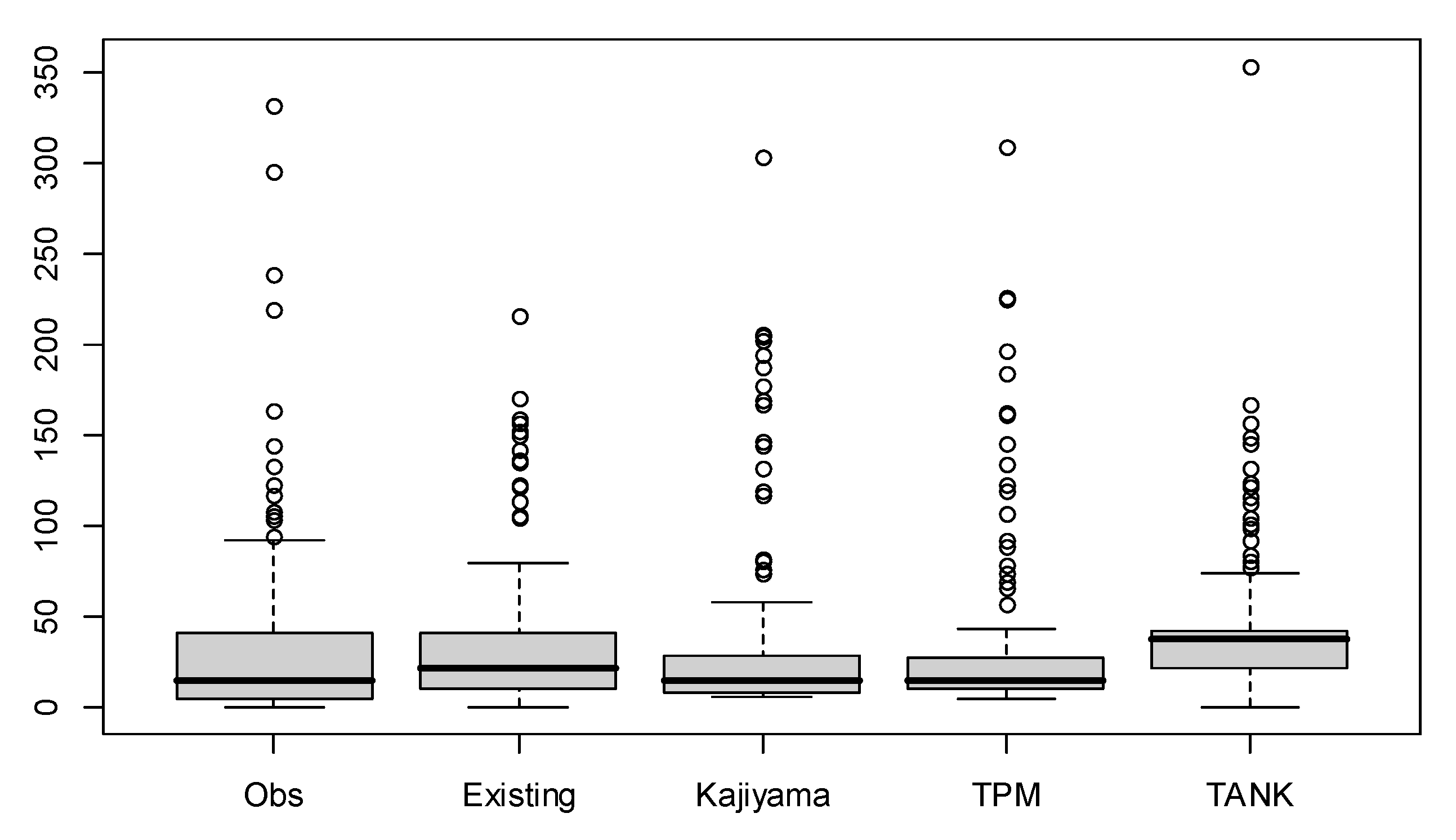
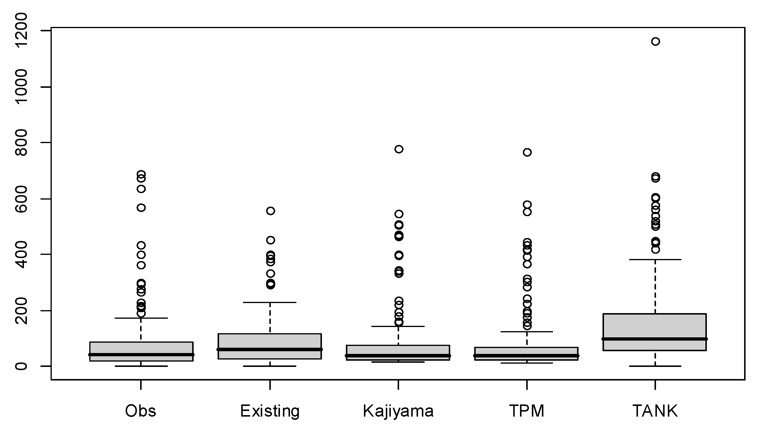
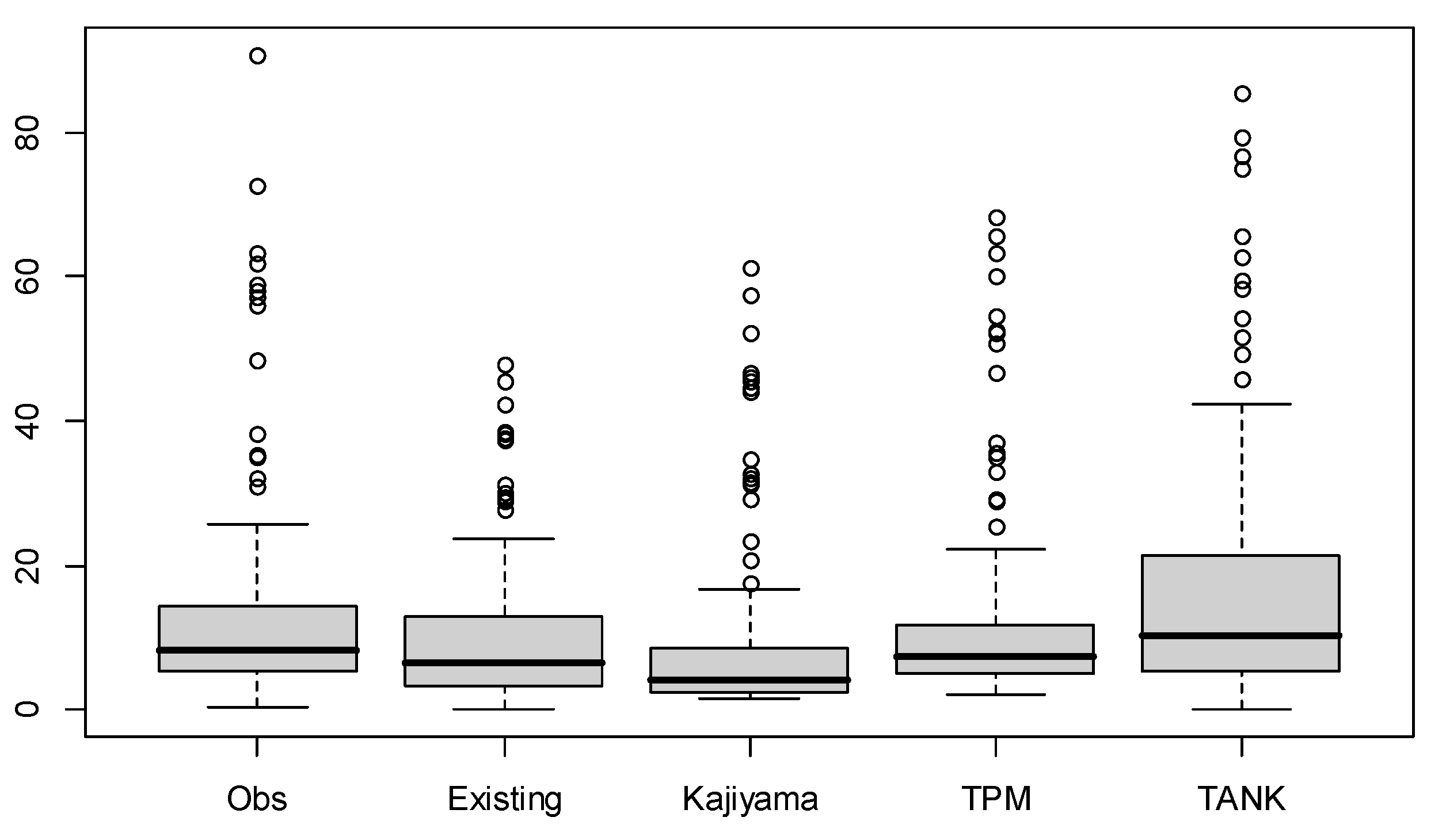
3.3. Comparison and Analysis of the Monthly Runoff Simulation Results

Table 6 shows the comparison of the measured discharge values with the discharge simulated using four basin runoff simulation methods in the Jeongseon basin where the Deoksong SHP plant is located. To evaluate whether the discharge was simulated accurately, the distribution of the discharge was compared through the quartiles and evaluation indicators of root mean square error (RMSE), Nash–Sutcliffe efficiency (NSE), and R2. It means that the distribution of the simulated discharge is accurate as the distribution and the error of the measured discharge decreases. The result of comparing the distribution of average monthly discharge is shown in Figure 2 below. Each index is represented by Equations (14)–(16). If the RMSE is closer to 0, and the NSE and R2 are closer to 1, it means the simulation is more accurate.
R M S E   =   ( O t M t ) 2 n
N S E   =   1 ( O t M t ) 2 ( O t O t ¯ ) 2
R 2   =   ( M t O t ¯ ) 2 ( O t O t ¯ ) 2
where O t is the measured value; M t is the simulated values; and n and O t ¯ are the number of data and the average value of measured value, respectively. The discharge values simulated using the modified TPM showed a low error of the mean, the smallest RMSE value, and the largest R 2 value. Thus, the modified TPM best simulated the measured discharge. Furthermore, when the distribution of the discharge data was compared, the results of the conventional method and the Kajiyama formula also reflected the overall distribution of the measured discharge well. In contrast, the Tank model showed the largest difference between the simulated and measured discharge data.
The discharge simulation results using the four basin runoff simulation methods for the Saigokcheon junction basin where the Hanseok SHP plant is located are shown in Table 7. The result of comparing the distribution of average monthly discharge is shown in Figure 3. The discharge simulated using the modified TPM showed a small error of the mean and the smallest RMSE. The Nash–Sutcliffe efficiency factor and R2 values were the largest for the results of the conventional method and the Kajiyama formula, respectively. The results of the Kajiyama formula and modified TPM reflected the overall distribution of the measured discharge values well. In contrast, the Tank model showed the largest difference between the simulated and measured discharge values.
The discharge simulation results using the four basin runoff simulation methods for the Socheon streamflow station basin where the Socheon SHP plant is located are shown in Table 8. The results of comparing the distribution of average monthly discharge are shown in Figure 4. The discharge simulated using the modified TPM showed a small error of the mean, the smallest RMSE, and the largest Nash–Sutcliffe efficiency factor and R2 values. Thus, the modified TPM provided the most accurate simulation of the discharge values. Overall, the simulated discharge values were underestimated. The Tank model showed the largest difference between the simulated and measured discharge values.

3.4. Application of the Blending Technique

The discharge values simulated using four basin runoff simulation methods in the same basin showed different patterns depending on the basin characteristics and the instability of the models. To address the uncertainties in the simulation results, blending techniques are typically applied. In this study, discharge values were calculated by applying the simple average method, MMSE, SMA, and MSE as blending techniques. For this calculation, the discharge results simulated using the Tank model, which showed relatively low accuracy in all basins, were excluded.
The comparison of the measured discharge values with the runoff results obtained by applying the blending techniques to the simulated discharge values in the Jeongseon basin where the Deoksong SHP plant is located are shown in Table 9. The results of the three blending techniques except the MMSE technique showed a smaller RMSE value and larger Nash–Sutcliffe efficiency factor and R 2 than the simulation results of the individual models. The time series graph drawn by excluding the result of applying the MMSE technique, which was significantly different from the results (Figure 5a), shows that all the values were similar to the measured discharge values.
The comparison of the measured discharge values with the runoff results obtained by applying the blending techniques to the simulated discharge values in the Saigokcheon junction basin where the Hanseok SHP plant is located are shown in Table 10. The results of the MMSE technique were excluded from the analysis because of the negative discharge values. Similar to the results of the Jeongseon basin, the results of the three blending techniques, except for the MMSE technique, showed a smaller RMSE value and larger Nash–Sutcliffe efficiency factor and R 2 than the results of the individual models. The time series graph drawn by excluding the result of applying the MMSE technique (Figure 5b) shows that all the values were similar to the measured discharge values, except for some underestimated sections.
The comparison of the measured discharge values with the runoff results obtained by applying the blending techniques to the simulated discharge values in the Socheon streamflow station basin where the Socheon SHP plant is located are shown in Table 11. The results of the Socheon streamflow station basin also showed a smaller RMSE than the simulation result of individual models except for the MMSE technique. The TPM simulation results showed slightly larger values of the Nash–Sutcliffe efficiency factor and R2 (0.85 and 0.88, respectively), but when the blending techniques were applied, the Nash–Sutcliffe efficiency factor and R2 were generally larger. The time series graph drawn by excluding the result of the MMSE technique (Figure 5c) showed smaller differences between the results of the blending techniques, unlike the large differences between the individual simulation results.
When the runoff was calculated by applying the blending techniques to the simulated discharge values, the results were improved compared to the simulation results of the individual models. When the discharge values calculated by applying the blending techniques were compared, the calculated discharge values were almost identical, except for the MMSE technique. Therefore, the flow-duration characteristics method, Kayajima formula, and modified-TPM method should be used to simulate discharge to estimate the SHP potential of an ungaged basin. Furthermore, since the simulated runoff results were different for each method, one of the three blending techniques (simple average method, SMA, and MSE) should be applied. The mean of the measured discharge values is required when applying the MMSE and SMA techniques. Since the discharge results were almost identical when four blending techniques were applied, the simple average method or MSE should be used to calculate the discharge in an ungaged basin.

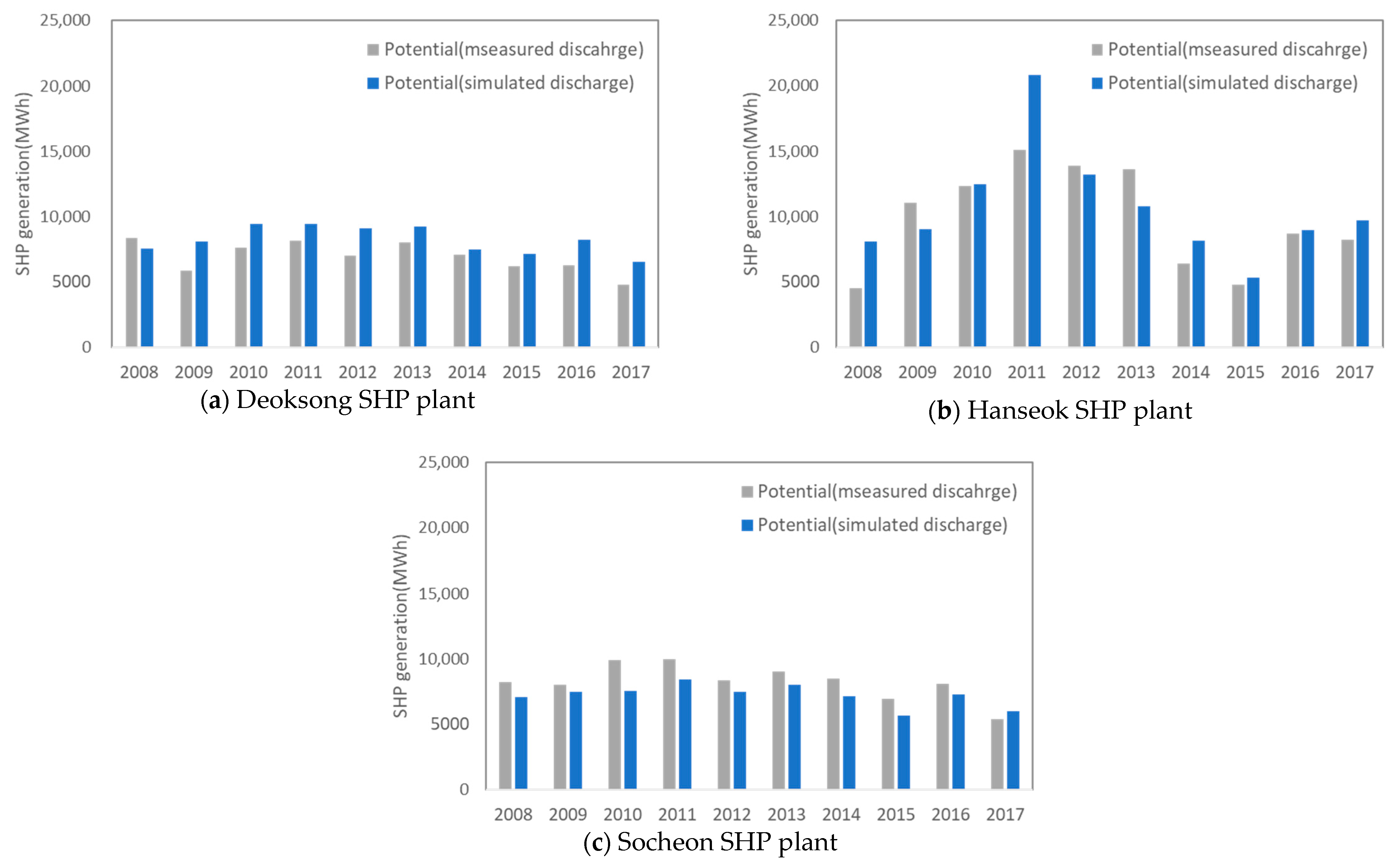
3.5. Calculation of SHP Potential

The power generation potential of each SHP plant was calculated by applying the equation to the discharge data calculated using the methods described in Section 3.4. The runoff result obtained by applying the MSE blending technique, which produced the most accurate discharge values in each basin, was used. The characteristics of each SHP plant presented in Table 1 were used in the calculations. The water turbine efficiency of 0.4 and generator efficiency of 0.8 were used when no known values existed. However, to improve accuracy, the actual efficiency was estimated by comparing the past monthly generation data of each plant with the simulated theoretical potential.
The annual SHP potential of three target SHP plants was calculated by applying the measured discharge data collected from the stage stations and the simulated discharge values. The calculated SHP potential and the actual generation data (annual generation data for 2008–2010 disclosed by each plant) of each SHP plant were compared (Figure 6).
In the Deoksong SHP plant, the potential calculated using the measured discharge data showed an error range of 7.0–33.4% relative to the actual generation, and the potential calculated using the simulated discharge showed an error range of 4.0–28.6% (Table 12). In general, the trends of the measured and simulated discharge were similar, and the potential was estimated more accurately when the estimated actual efficiency was applied. In the Hanseok SHP plant, the potential estimated using the measured discharge data showed an error range of 29.7–60.9% relative to the actual generation. The potential estimated using the simulated discharge data showed an error range of 24.1–31.5%, and thus it was closer to the actual generation than the potential estimated using the measured discharge data (Table 13). In the Socheon SHP plant, the potential estimated using the measured discharge data showed an error range of 12.5–51.7% relative to the actual generation, and the potential estimated using the simulated discharge showed an error range of 7.1–31.6% (Table 14).
Since the potential has a trend of being slightly overestimated than the actual generation, the efficiency applied when calculating the power generation potential was larger than the generator efficiency of an actual power plant. When it is difficult to accurately estimate the efficiency of a generator, the efficiency of 0.32 is typically used with a water turbine efficiency of 0.4 and a generator efficiency of 0.8. However, in this study, the efficiency was calculated during the period of the available actual generation data and the mean efficiency was used. More accurate potential estimates can be derived by applying the mean efficiency rather than by applying the same efficiency of 0.32. Therefore, if the accurate actual efficiency of each plant is known, more accurate SHP potentials can be estimated using the simulated discharge data, even in ungaged basins.

4. Conclusions

Interest in SHP generation has been increasing along with the need for new and renewable energy resources. Unlike the renewable energy sources for which the power generation potential is calculated based on meteorological data (solar and wind power) and radar data, the hydropower generation potential is estimated using the river discharge data. In gaged basins, the power generation potential can be estimated using the measured discharge, but in ungaged basins, the discharge must be simulated or calculated using an empirical formula or a discharge model. The discharge estimation results vary depending on the formula or model used. Nevertheless, using various models can produce more reliable discharge values and more accurate estimations of power generation potential by reducing the errors, which may be large when only one model is used. This study estimated the discharge values using the flow-duration characteristics model, Kajiyama formula, modified TPM, and the Tank model. In addition, four blending techniques (simple average method, MMSE, SMA, and MSE) were used to minimize the uncertainties in the discharge values. The results of this study can be summarized as follows.
  • Discharge simulation using various runoff estimation models: In addition to the flow-duration characteristics model, which is used to simulate discharge for the estimation of the SHP potential, this study also applied the Kayajima formula, modified TPM, and the Tank model. These runoff estimation methods are representative methods applied in numerous discharge estimation studies in the field of hydrology. The applicability of the modified TPM, which is a modification of the existing TPM method, was verified in this study for the first time. The runoff estimation methods were verified by comparing the simulated discharge values with the measured discharge values in each basin. The discharge values simulated by applying the modified TPM method in three target SHP plant basins of Deoksong, Hanseok, and Socheon showed the smallest error of the mean and RMSE relative to the measured discharge data and the largest Nash–Sutcliffe efficiency factor and R2 values. Thus, the modified TPM method was the most accurate method. The distribution of the discharge values simulated using the Kajiyama formula and the flow-duration characteristics model reflected the distribution of the measured discharge values. However, unlike the other methods, the Tank model showed the largest differences between the simulated and measured discharge values.
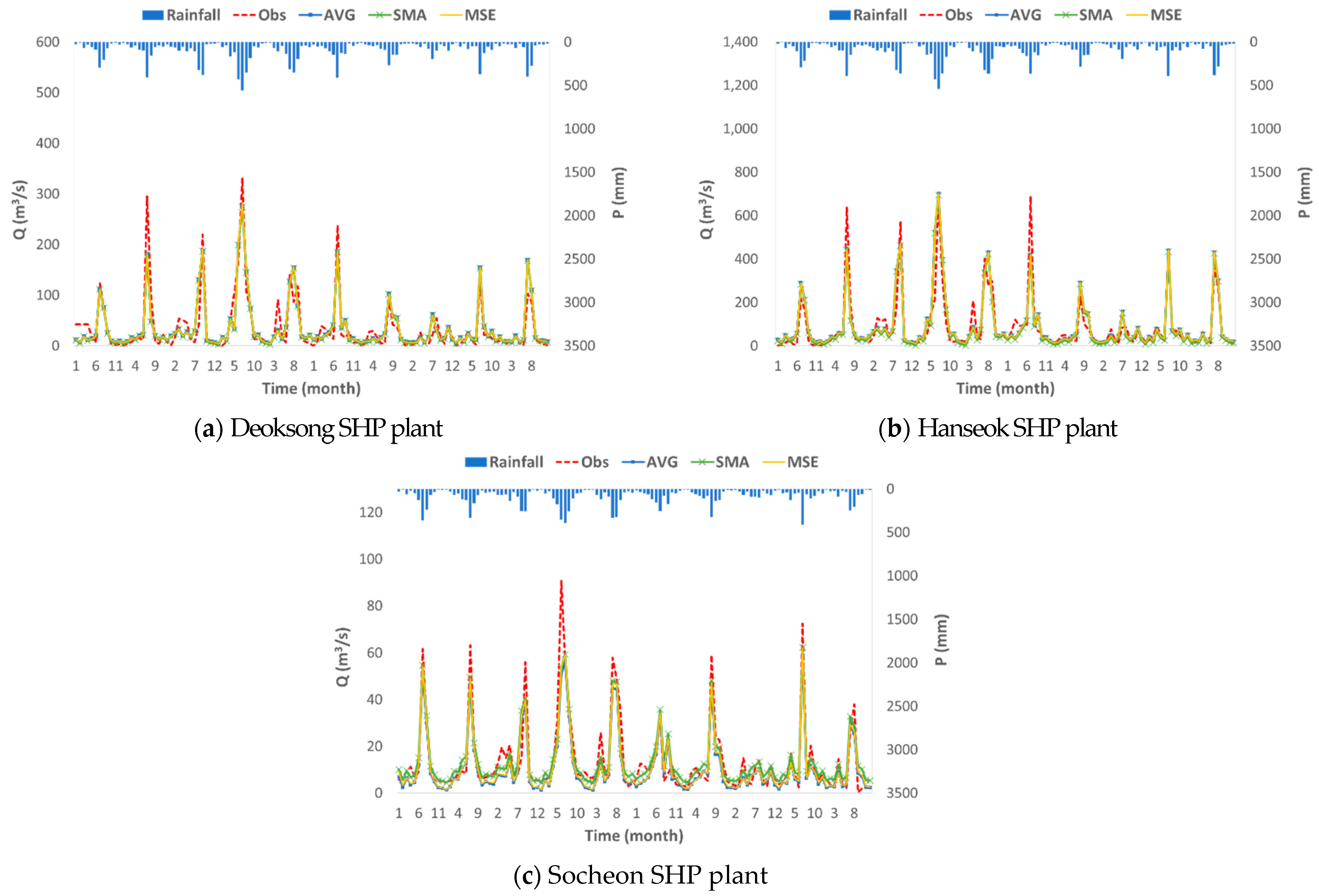
  • Application of blending techniques: When discharge is simulated using various runoff estimation methods, different simulated discharge values are obtained depending on the method. To address the uncertainties in the runoff simulation results, blending techniques were applied to the runoff estimations excluding the less accurate results of the Tank model. The blending techniques of the simple average method, MMSE, SMA, and MSE were applied. The comparison of the blending results of the simulated discharge values with the measured discharge values showed that the MMSE method produced results that were significantly different from the measured discharge values. The distribution of the discharge values estimated by the three blending techniques except for MMSE were almost identical to the distribution of the measured discharge values. Therefore, applying one of the three blending techniques (simple average method, SMA, and MSE) is appropriate for accurate runoff estimation. In ungaged basins, which do not have measured discharge values, the MSE technique is considered the best method.
This study validated the applicability of the proposed methodology for the estimation of the SHP potential in ungaged basins that do not have discharge data. To date, the discharge has typically been obtained using the flow-duration characteristics model, but this study proposed various discharge estimation models for the accurate estimation of the power generation potential and demonstrated that the uncertainty of the models could be reduced using blending techniques. This study also suggests that the MSE method is the best blending technique for estimating the discharge in ungaged basins. Therefore, the results of this study can be used as a standard methodology for estimating the SHP energy potential with higher accuracy and reliability. Furthermore, more accurate calculation of the future plant capacity based on the future energy potential will contribute to minimizing the costs of the initial installation and maintenance of hydropower plants.

Author Contributions

Conceptualization, H.K.; Methodology, J.J.; Software, J.K., H.J. and S.J.; Validation, Y.B.; Formal analysis, J.J.; Investigation, J.K.; Resources, S.J.; Data curation, S.J.; Writing—original draft preparation, J.J.; Writing—review and editing, S.J. and H.K.; Visualization, J.J.; Supervision, H.K.; Project administration, H.J.; Funding acquisition, Y.B. All authors have read and agreed to the published version of the manuscript.

Funding

This research was funded by the National Research Foundation of Korea (NRF) grant funded by the Korea government (MSIT), grant number 2017R1A2B3005695.

Institutional Review Board Statement

Not applicable.

Informed Consent Statement

Not applicable.

Acknowledgments

This research was supported by the National Research Foundation of Korea (NRF) grant funded by the Korea government (MSIT) (no. 2017R1A2B3005695).

Conflicts of Interest

The authors declare no conflict of interest.

References

  1. Frey, G.W.; Linke, D.M. Hydropower as a renewable and sustainable energy resource meeting global energy challenges in a reasonable way. Energy Policy 2002, 30, 1261–1265. [Google Scholar] [CrossRef]
  2. Tondi, G.; Chiaramonti, D. Small hydro in Europe help meets the CO2 target. Int. Water Power Dam Constr. 1999, 51, 36–40. [Google Scholar]
  3. Silva, E.I.L.; Silva, E.N.S. Handbook on: Small Hydropower Development and Environment: A Case Study on Sri Lanka; Water Resources Science and Technology: Ragama, Sri Lanka, 2016. [Google Scholar]
  4. Korea Energy Agency. 2020. Available online: http://www.kemco.or.kr/ (accessed on 1 September 2020).
  5. Razan, J.I.; Islam, R.S.; Hasan, R.; Hasan, S.; Islam, F. A Comprehensive Study of Micro-Hydropower Plant and Its Potential in Bangladesh; ISRN Renewable Energy: London, UK, 2012. [Google Scholar]
  6. Ministry of Trade, Industry and Energy. New & Renewable Energy White Paper in 2018, Korea; Ministry of Trade, Industry and Energy: Sejong, Korea, 2018.
  7. Adhau, S.P.; Moharil, R.M.; Adhau, P.G. Mini-hydropower Generation on Existing Irrigation Projects: Case Study of Indian Sties. Renew. Sustain. Eenrgy Rev. 2012, 16, 4785–4795. [Google Scholar] [CrossRef]
  8. Larentis, D.G.; Collischonn, W.; Olivera, F.; Tucci, C.E.M. Gis-based Procedures for Hydropower Potential Spotting. Energy 2010, 35, 4237–4243. [Google Scholar] [CrossRef]
  9. Yu, I.; Kim, H.; Jeong, S. Estimation of Annual Small Hydro-powerof Standard Basin in Korea. J. Korean Soc. Hazard Mitig. 2017, 17, 473–481. [Google Scholar] [CrossRef]
  10. Kim, K.; Yi, C.; Lee, J.; Shim, M. Framework for Optimum Scale Determination for Small Hydropower Development Using Economic Analysis. J. Korea Water Resour. Assoc. 2007, 2007, 3367–3370. [Google Scholar]
  11. Park, W.; Lee, C. Estimation Method of Small Hydro Power Potential Using a Resource Map. Proc. Korean Sol. Energy Soc. 2008, 11, 322–326. [Google Scholar]
  12. Park, W.; Lee, C. Analysis of Small Hydropower Resource Characteristics for Nakdong River System. J. Korean Sol. Energy Soc. 2012, 32, 68–75. [Google Scholar] [CrossRef] [Green Version]
  13. Park, J.; Park, C.; Lee, W.; Kim, J. A Study on Analyzing Efficiency of Small Hydropower Plant. Proc. Korean Soc. Civil Eng. 2010, 10, 1989–1992. [Google Scholar]
  14. Cho, T.; Kim, Y.; Lee, K. Improving Low Flow Estimation for Ungauged Basins in Korea. J. Korean Sol. Energy Soc. 2016, 36, 39–47. [Google Scholar]
  15. Park, N.; Park, S.; Choi, D.; Kim, H.; Kang, Y. Business Model of Renewable Energy Resource Energy Resource Map. J. Korean Sol. Energy Soc. 2016, 36, 39–47. [Google Scholar] [CrossRef] [Green Version]
  16. Chalise, S.R.; Kansakar, S.R.; Rees, G.; Croker, K.; Zaidman, M. Management of water resources and low flow estimation for the Himalayan basins of Nepal. J. Hydrol. 2003, 282, 25–35. [Google Scholar] [CrossRef]
  17. Noyes, R. Small and Micro Hydro Electric Power Plants: Technology and Feasibility; Energy Technology Review, No. 60; Noyes Data Corperation: Park Ridge, NJ, USA, 1980. [Google Scholar]
  18. Park, W.; Lee, C. The Effects of Design Parameters for Small Scale Hydro Power Plant with Rainfall Condition. J. Korean Sol. Energy Soc. 2008, 28, 43–49. [Google Scholar]
  19. Gossain, A.K.; Rao, S. Small hydropower assessment using GIS and hydrological modeling-Nagaland case study. In Proceedings of the National Seminar on Renewable Energy and Energy Management Organized by North Eastern Regional Institute of Water and Land Management, Tezpur, India, 23–24 August 2005. [Google Scholar]
  20. Kusre, B.C.; Baruah, D.C.; Bordoloi, P.K.; Patra, S.C. Assessment of hydropower potential using GIS and hydrological modeling technique in Kopili River basin in Assam (India). Appl. Energy 2010, 87, 298–309. [Google Scholar] [CrossRef]
  21. Thin, K.K.; Zin, W.W.; San, Z.M.; Kawasaki, L.T.; Moiz, A.; Bhagabati, S.S. Estimation of Run-of-River Hydropower Potential in the Myitnge River Basin. J. Disaster Res. 2020, 15, 267–276. [Google Scholar] [CrossRef]
  22. Park, W.; Lee, C. Analysis on Design Parameters of Small Hydropower Sites with Rainfall Conditions. J. Korean Sol. Energy Soc. 2012, 32, 59–64. [Google Scholar]
  23. Cheng, C.T.; Miao, S.M.; Luo, B.; Sun, Y.J. Forecasting monthly energy production of small hydropower plants in Ungaged basins using grey model and improved seasonal index. J. Hydroinform. 2017, 19, 993–1008. [Google Scholar] [CrossRef] [Green Version]
  24. Zlatanović, N.; Stefanović, M.; Milojević, M.; Čotrić, J. Automated hydrologic analysis of ungaged basins in Serbia using open source software. Water Pract. Technol. 2014, 9, 445–449. [Google Scholar] [CrossRef]
  25. Saliha, A.H.; Awulachew, S.B.; Cullmann, J.; Horlacher, H.B. Estimation of flow in ungaged catchments by coupling a hydrological model and neural networks: Case study. Hydrol. Res. 2011, 42, 386–400. [Google Scholar] [CrossRef]
  26. Kim, J.G.; Sun, H.; Kim, J.; Yun, C.; Kim, H.G.; Kang, Y.; Kang, B. Estimation of Nationwide Mid-sized Basin Unit Small Hydropower Potential Using Grid-based Surface Runoff model. New Renew. Energy 2018, 14, 12–19. [Google Scholar] [CrossRef]
  27. Kim, G.H.; Sun, S.P.; Yeo, G.D.; Kim, H.S. A Study on Variability of Small Hydro Power Generation Considering Climate change. Proc. KSCE Korean Soc. Civil Eng. 2012, 10, 932–935. [Google Scholar]
  28. Arriagada, P.; Dieppois, B.; Sidibe, M.; Link, O. Impacts of Climate Change and Climate Variability on Hydropower Potential in Data-Scarce Regions Subjected to Multi-Decadal Variability. Energies 2019, 12, 2747. [Google Scholar] [CrossRef] [Green Version]
  29. Carvajal, P.E.; Anandarajah, G.; Mulugetta, Y.; Dessens, O. Assessing uncertainty of climate change impacts on long-term hydropower generation using the CMIP5 ensemble—The case of Ecuador. Clim. Chang. 2017, 144, 611–624. [Google Scholar] [CrossRef] [Green Version]
  30. Chilkoti, V.; Bolisetti, T.; Balachandar, R. Climate change impact assessment on hydropower generation using multi-model climate ensemble. Renew. Energy 2017, 109, 510–517. [Google Scholar] [CrossRef]
  31. Eshchanov, B.; Abylkasymova, A.; Overland, I.; Moldokanov, D.; Aminjonov, F.; Vakulchuk, R. Hydropower Potential of the Central Asian Countries. Cent. Asia Reg. Data Rev. 2019, 19, 1–7. [Google Scholar]
  32. Hu, Y.; Jin, X.; Guo, Y. Big data analysis for the hydropower development potential of ASEAN-8 based on the hydropower digital planning model. J. Renew. Sustain. Energy 2018, 10, 034502. [Google Scholar] [CrossRef]
  33. Hamududu, B.H.; Killingtveit, Å. Hydropower production in future climate scenarios; the case for the Zambezi River. Energies 2016, 9, 502. [Google Scholar] [CrossRef] [Green Version]
  34. Burgan, H.I.; Aksoy, H. Monthly flow duration curve model for ungauged river basins. Water 2020, 12, 338. [Google Scholar] [CrossRef] [Green Version]
  35. Atieh, M.; Taylor, G.; Sattar, A.M.; Gharabaghi, B. Prediction of flow duration curves for ungauged basins. J. Hydrol. 2017, 545, 383–394. [Google Scholar] [CrossRef]
  36. Worland, S.C.; Steinschneider, S.; Asquith, W.; Knight, R.; Wieczorek, M. Prediction and Inference of Flow Duration Curves Using Multioutput Neural Networks. Water Resour. Res. 2019, 55, 6850–6868. [Google Scholar] [CrossRef] [Green Version]
  37. Kim, S.; Hong, S.J.; Kang, N.; Noh, H.S.; Kim, H.S. A comparative study on a simple two-parameter monthly water balance model and the Kajiyama formula for monthly runoff estimation. Hydrol. Sci. J. 2016, 61, 1244–1252. [Google Scholar] [CrossRef]
  38. Yoon, Y.N. Engineering Hydrology; Chung Moon Kak: Paju, Korea, 1998. [Google Scholar]
  39. Xiong, L.; Guo, S. A two-parameter monthly water balance model and its application. J. Hydrol. 1999, 1999, 111–123. [Google Scholar] [CrossRef]
  40. Brutsaert, W.; Sugita, M. Application of self-preservation in the diurnal evolution of the surface energy budget to determine daily evaporation. J. Geophys. Res. Atmos. 1992, 97, 18377–18382. [Google Scholar] [CrossRef]
  41. Sugawara, M. On the analysis of runoff structure about several Japanese rivers. Jpn. J. Geophys. 1961, 2, 1–76. [Google Scholar]
  42. Jung, S. Estimation and Future Prospect of Small Hydropower Generation Potential for the Ungaged Basin. Ph.D. Thesis, Inha University, Incheon, Korea, 2020. [Google Scholar]
  43. Lee, M.; Kang, N.; Joo, H.; Kim, H.S.; Kim, S.; Lee, J. Hydrological Modeling Approach Using Radar-Rainfall Ensemble and Multi-Runoff-Model Blending Technique. Water 2019, 11, 850. [Google Scholar] [CrossRef] [Green Version]
  44. Georgakakos, K.P.; Seo, D.J.; Gupta, H.; Schaake, J.; Butts, M.B. Towards the characterization of streamflow simulation uncertainty through multimodel ensembles. J. Hydrol. 2004, 298, 222–241. [Google Scholar] [CrossRef]
  45. Li, W.; Sankarasubramanian, A. Reducing hydrologic model uncertainty in monthly streamflow predictions using multimodel combination. Water Resour. Res. 2012, 48, 48. [Google Scholar] [CrossRef] [Green Version]
  46. Krishnamurti, T.N.; Kishtawal, C.M.; Zhang, Z.; LaRow, T.; Bachiochi, D.; Williford, E. Multimodel ensemble forecasts for weather and seasonal climate. J. Clim. 2000, 13, 4196–4216. [Google Scholar] [CrossRef]
  47. Geem, Z.W.; Kim, J.H.; Loganathan, G.V. A new heuristic optimization algorithm: Harmony search. Simulation 2001, 76, 60–68. [Google Scholar] [CrossRef]
  48. Kim, J.H. Harmony search algorithm and its application to optimization problems in civil and water resources engineering. J. Korea Water Resour. Assoc. Korea Water Resour. Assoc. 2018, 51, 281–291. [Google Scholar]
  49. Paik, K.; Kim, J.H.; Kim, H.S.; Lee, D.R. A conceptual rainfall-runoff model considering seasonal variation. Hydrol. Process. Int. J. 2005, 19, 3837–3850. [Google Scholar] [CrossRef]
Figure 1. The taget basins, basin area, locations of small hydropower (SHP) plants, rainfall, and streamflow stations.
Energies 14 02977 g001
Figure 2. The distributions of the simulated and measured monthly average discharge by the simulation method for the Deoksong SHP plant (unit: m3/s).
Energies 14 02977 g002
Figure 3. The distributions of the simulated and measured monthly average discharge by the simulation method for the Hanseok SHP plant (unit: m3/s).
Energies 14 02977 g003
Figure 4. The distributions of the simulated and measured monthly average discharge by the simulation method for the Socheon SHP plant (unit: m3/s).
Energies 14 02977 g004
Figure 5. Comparison of the runoff blending results.
Energies 14 02977 g005
Figure 6. The comparison results between the simulated and measured SHP potential.
Energies 14 02977 g006
Table 1. Information on small hydropower (SHP) plants of target basins.
SHP PlantStandard BasinCommissioned TimeEffective Head
(m)
Power Generation Flow Rate
(m3/s)
Installed Power Associated with the Hydropower Plant (kW)
DeoksongJeongseonMarch, 199312.5 25.0 2600
HanseokSaigokcheon junctionMarch, 19983.8Avg. 3.02/Max.12.7 2214
SocheonSocheon streamflow stationAugust, 198522.5 12.5 2400
Table 2. General characteristics of basins.
Standard BasinLarge BasinRunoff Coefficient (C)Runoff Curve Number (CN)Basin Area
(km2)
Cumulative Basin Area (km2)
JeongseonHan River0.5658179.61834.7
Saigokcheon junctionHan River0.5664 128.7 4898.0
Socheon streamflow stationNakdong River0.5747 140.8 547.2
Table 3. Specifications of the rainfall stations.
Observation StationManagement AgencyCoordinates (WGS84)Start of Observation
LatitudeLongitude
YeongwolKorea Meteorological Administration
(KMA)
37.18128.461 December 1997
Daegwallyeong37.68128.7211 July 1971
Yeongju36.87128.5228 November 1972
Uljin36.99129.4112 January 1971
Bonghwa36.94128.911 January 1988
Table 4. Specifications of the streamflow station.
Observation StationManagement AgencyZero of Staff Gauge
(EL.m)
Benchmark Elevation
(EL.m)
Start of Observation
JeongseonMinistry of Environment296.79312.421 January 1918
YeongchunK-water159.97177.6330 August 1985
SocheonK-water250.08262.0316 July 1978
Table 5. Test results of the model parameters.
Standard BasincSC (mm)F2R2 (%)
Jeongseon0.77502.205.54E + 070.85
Saigokcheon junction0.75425.815.80E + 080.71
Socheon streamflow station 0.50519.717.31E + 060.77
Table 6. Comparison of the distributions and statistics of the simulated and measured monthly average discharge for the Deoksong SHP plant.
(Unit: m3/s)
Discharge Simulation MethodMeasured DischargeFlow-Duration Characteristics ModelKajiyama FormulaModified TPMTank Model
Minimum 0.00 0.70 5.28 4.77 0.61
First quartile 4.94 10.47 8.43 9.87 21.82
Median 14.35 21.60 14.33 14.90 37.58
Third quartile 39.97 41.52 28.85 27.37 41.87
Maximum 331.77 216.20 303.04 308.46 353.46
Mean 35.17 37.61 37.04 35.10 45.42
Standard deviation 56.32 43.01 55.46 52.44 44.30
RMSE - 28.32 25.57 24.12 66.13
Nash–Sutcliffe efficiency factor - 0.56 0.79 0.79 −1.25
R 2 - 0.76 0.80 0.82 0.03
Table 7. Comparison of the distribution and statistics of the simulated and measured monthly average discharge for the Hanseok SHP plant.
(Unit: m3/s)
Discharge Simulation MethodMeasured DischargeFlow Duration Characteristics ModelKajiyama FormulaModified TPMTank Model
Minimum 1.13 0.70 14.08 11.59 0.00
First quartile 20.68 27.43 22.69 22.85 57.18
Median 40.86 59.65 38.47 36.39 97.67
Third quartile 85.88 113.85 73.42 66.57 187.25
Maximum 688.81 559.00 777.74 767.85 1165.64
Mean 88.12 100.56 98.66 87.35 168.35
Standard deviation 132.76 113.76 145.65 132.18 183.93
RMSE - 64.14 63.66 61.83 121.61
Nash–Sutcliffe efficiency factor - 0.81 0.68 0.78 0.56
R 2 - 0.77 0.81 0.79 0.78
Table 8. Comparison of the distribution and statistics of the simulated and measured monthly average discharge for the Socheon SHP plant.
(Unit: m3/s)
Discharge Simulation MethodMeasured DischargeFlow Duration Characteristics ModelKajiyama FormulaModified TPMTank Model
Minimum 0.22 0.10 1.57 2.03 0.00
First quartile 5.27 3.25 2.49 4.90 5.43
Median 8.10 6.40 4.19 7.24 10.20
Third quartile 14.30 12.80 8.36 11.81 21.10
Maximum 90.75 47.90 61.27 68.28 85.61
Mean 13.98 10.24 9.52 12.84 17.43
Standard deviation 16.25 10.92 12.97 14.66 18.59
RMSE - 8.59 7.75 5.71 9.14
Nash–Sutcliffe efficiency factor - 0.38 0.64 0.85 0.76
R2 - 0.83 0.86 0.88 0.79
Table 9. Comparison of the distribution and statistics of the runoff blending results for the Deoksong SHP plant.
(Unit: m3/s)
Discharge Simulation MethodMeasured DischargeSimple Average MethodMMSESMAMSE
Minimum 0.00 4.00 −63.70 2.60 4.20
First quartile 4.94 10.10 −44.75 8.70 10.43
Median 14.35 17.70 −20.35 16.25 17.00
Third quartile 39.97 31.80 22.45 30.40 30.75
Maximum 331.77 275.90 745.70 274.50 281.00
Mean 35.17 36.58 35.17 35.17 36.46
Standard deviation 56.32 49.83 148.87 49.83 50.39
RMSE 24.56 100.88 24.52 24.39
Nash–Sutcliffe efficiency factor 0.76 0.54 0.76 0.76
R2 0.81 0.81 0.81 0.81
Table 10. Comparison of the distributions and statistics of the runoff blending result for the Hanseok SHP plant.
(Unit: m3/s)
Discharge Simulation MethodMeasured DischargeSimple Average MethodMMSESMAMSE
Minimum 1.13 9.70 −149.00 2.30 9.80
First quartile 20.68 26.98 −100.15 19.57 27.00
Median 40.86 46.50 −45.60 39.10 46.15
Third quartile 85.88 82.42 56.92 75.03 81.88
Maximum 688.81 701.50 1725.50 694.10 703.50
Mean 88.12 95.52 88.12 88.12 95.34
Standard deviation 132.76 129.18 350.94 129.18 129.29
RMSE 58.71 237.54 58.24 58.68
Nash–Sutcliffe efficiency factor 0.79 0.54 0.80 0.79
R2 0.81 0.81 0.81 0.81
Table 11. Comparison of the distributions and statistics of the runoff blending result for the Socheon SHP plant.
(Unit: m3/s)
Discharge simulation MethodMeasured DischargeSimple Average MethodMMSESMAMSE
Minimum 0.22 1.30 −20.10 4.40 1.50
First quartile 5.27 3.60 −11.90 6.70 3.98
Median 8.10 6.15 −2.35 9.25 6.35
Third quartile 14.30 11.35 16.55 14.45 11.20
Maximum 90.75 59.10 182.90 62.30 61.80
Mean 13.98 10.86 13.98 13.98 11.35
Standard deviation 16.25 12.75 44.79 12.75 13.28
RMSE 6.98 30.07 6.25 6.53
Nash–Sutcliffe efficiency factor 0.70 0.55 0.76 0.76
R2 0.87 0.87 0.87 0.88
Table 12. Annual SHP potential result for the Deoksong SHP plant.
YearSHP Actual Generation
(MWh)
SHP Potential (MWh)Deviation
( Actual   Generation     Potential Actual   Generation )
Measured DischargeSimulated DischargeMeasured DischargeSimulated Discharge
2008628883917571−33.4%−20.4%
20096295585380987.0%−28.6%
201090327625943315.6%−4.4%
2011 81319475
2012 70409079
2013 80439260
2014 71097508
2015 62317182
2016 63038226
2017 47666573
Table 13. Annual SHP potential result for the Hanseok SHP plant.
YearSHP Actual Generation
(MWh)
SHP Potential (MWh)Deviation
( Actual   Generation     Potential Actual   Generation )
Measured DischargeSimulated DischargeMeasured DischargeSimulated Discharge
200865234512809230.8%−24.1%
2009686011,0389019−60.9%−31.5%
2010950912,33412,453−29.7%−31.0%
2011 15,06620,824
2012 13,89713,185
2013 13,58910,760
2014 64208145
2015 47485315
2016 87088963
2017 81889690
Table 14. Annual SHP potential result for the Socheon SHP plant.
YearSHP Actual Generation
(MWh)
SHP Potential (MWh)Deviation
( Actual   Generation     Potential Actual   Generation )  
Measured DischargeSimulated DischargeMeasured DischargeSimulated Discharge
2008659981947066−24.2%−7.1%
2009565680157446−41.7%−31.6%
2010880499097575−12.5%14.0%
2011 99618396
2012 83867460
2013 90248020
2014 84677124
2015 69605672
2016 80967306
2017 54176017
Publisher’s Note: MDPI stays neutral with regard to jurisdictional claims in published maps and institutional affiliations.

