Abstract
Optimal performance parameters must be found in order to organize efficient heat and mass transfer and effective flue gas cooling using a wet scrubber. Mathematical models are widely used for system optimization. However, a significant number of the available models have application limitations. This study presents a universal model for heat and mass transfer simulation in a scrubber called a fog unit, which has been developed and validated. Validation was performed by comparing the experimental and calculated results. Good agreement was achieved among the data, with differences between results not exceeding 10%. The model facilitates an investigation of the effects of gas flow, droplet size, and sprayed water on heat recovery from flue gas. An experimental matrix for fog unit capacity which included five main variables was designed and analyzed. The boundaries of the parameters are set considering the results of the experiments. The optimization method used is the path of the steepest ascent. The obtained results show the parameter change steps to achieve higher capacity of the condenser. In the studied unit, the maximum condenser capacity is limited by a flue gas flow value of 0.01 Nm3/s. The condenser optimization study that was conducted is viewed as a basis for further studies.
1. Introduction
There are several environmental benefits resulting from the use of biomass for heating purposes in households. One of the bigger advantages is that biomass is a CO2-neutral fuel. It is possible to reduce greenhouse gas emissions by replacing existing heating plants with the use of natural gas. At the same time, the use of biomass to generate heat also has its drawbacks, among which particulate matter (PM) is a major issue [1]. PM is a significant problem in the world [2]. Nowadays, the PM emission values in flue gas are controlled mainly in medium- and high-power boilers.
There is a lack of common standards and regulations regarding PM control from small capacity boilers which are widely used in households. Some of the existing standards are not strict enough and the permissible PM limits in the flue gas are too high [3].
The EU Eco-design Directive 2009/125/EK [4] ensures the unique requirements for low capacity boilers. The boilers have a requirement for a minimum energy efficiency of 75% or 77% depending on the boiler type, as well as a maximum allowed PM concentration, with an automatic fuel supply of 40 and 60 mg/m3 for manual fuel supply boilers.
There are many flue gas treatment technologies for PM concentration reduction. Applied treatment technologies can be divided into two categories, i.e., dry and wet methods. A study by Bianchini et al. [5] described, in detail, the operational principles of the various PM treatment technologies, their advantages, and their disadvantages.
Nowadays, scrubbers are widely applied for PM treatment in different energy sources, in industrial and manufacturing objects. Scrubbers can be characterized by high PM capture efficiency. In addition, there is the possibility of recovering heat from the outgoing flue gas to increase the energy efficiency of the combustion process, which is a major advantage of a scrubber. However, in order to make full use of it, it is important to ensure efficient heat and mass transfer processes between the flue gases and the water injected at the scrubber.
Typically, the largest heat losses for boilers are from outgoing flue gases which are mostly 5–10% and the heat losses mainly depend on the temperature of flue gas and air consumption [6]. There are cases when heat losses from outgoing flue gases exceed 15% [7]. Worldwide, there is a high potential for recovering heat energy from flue gases. In China. Calculations have shown that only 2538.8 trillion kJ of energy is lost with flue gases. Due to the heat recovery it would be possible to save approximately 100 million tons of coal [8].
In scrubbers, there is a direct contact heat exchange between hot flue gases and cold water. Direct contact heat exchange is a process, in which two substances with different temperatures interact with each other. Heat conduction is caused by the interaction of molecules in the substance as a result of a temperature gradient. In order to ensure effective recovery of heat from flue gases with scrubbers, it is important to organize heat and mass transfer. Evaporative or condensing processes, convection, and heat conduction can take place in scrubbers depending on the operating parameters and environmental conditions. Overall, the expression of these processes, as well as the heat recovery processes are influenced by more than 15 variable parameters [9].
The potential for deeper cooling and greater recovery of heat energy is also increased by increasing the water flow rate for spraying into flue gases [10]. The more effective process of heat transfer between flue gases and sprayed water can be achieved by reduction of the water temperature. At the same time, there is a certain optimum regarding the outgoing temperature of flue gases, in the range of up to 30 °C. After reaching this temperature, the future temperature decrease of the spray water is not economically viable [11].
Water spraying in scrubbers is organized in different ways. Depending on the applied technology, water is sprayed with various diameters and surface area of water droplets. The diameter of water droplets significantly influences heat transfer from flue gases to sprayed water. In addition, essential factors that determine heat exchange processes are initial velocity provided for droplets, droplet dispersity, and specifics of droplets [12].
Without optimizing the performance of scrubbers, there can be many consequences, for example, formation of water film on scrubber walls. As a result, a substantial amount of sprayed water flows on the scrubber walls, reducing total surface area of sprayed water droplets and not ensuring the effective heat exchange between gases and water [13]. As a result of spraying too much water, the flow of flue gases out of a scrubber’s reactor can be interrupted. In addition, this type of scrubber activity is not economically viable due to the increased electricity used for water spraying, while the amount of recovered heat energy is practically the same [14]. The effects of the pressure drop on heat and mass transfer must also be taken into account [15].
An optimization of a shell and tube district heating condenser was done by Saari et al. [16]. A complex investigation to find the optimal solution between heat transfer area, pressure drop, volume of the shell, and tube number was done using the developed model. The optimal sprayed water flow rate depending on the water temperature was determined. The difference in injected water flow rate with temperature change was nonlinear with a rapid decrease at first, and then more slowly as time passed [17].
During experimental research, due to specific environmental circumstances there are often limitations to determine temperatures, flow rate, directions, and other parameters. In order to find such possibilities, it is necessary to buy expensive measuring equipment and this significantly increases the cost of the research. In addition, modeling programs have an option to obtain results at specific values of variable parameters. In the case of experimental research, particularly in industrial experiments, it is sometimes difficult to achieve the values of the required parameters and there is a certain error [18].
Dynamic modeling of heat and mass processes is widely used for heat exchanger design development [19]. A physical and mathematical model of complex heat and mass transfer and condensation-absorption processes in a scrubber was developed and presented in a study by Shilyaev [20]. The model was based on experimental data and could be used for optimization of scrubber performance depending on construction and operation parameters. The role of water droplets was effectively investigated in the developed model.
Two numerical models were developed to investigate heat recovery from flue gases by Macháčková [21]. The first mathematical model was a stationary one-dimensional (1D) model based on the Colburn–Hougen model. The second model was a three-dimensional (3D) multiphase flow model based on the Euler model of mixture expanded by the model of condensation of water vapor from the flue gases. Both models were validated with experimental results, showed good correlation, and could be used for heat and mass transfer process simulation.
A model to research droplet nucleation and growth is found in [22]. Such a model was used to investigate droplet distribution based on the Poisson point process, the spatial distribution of droplets using Ripley’s L function method, as well as to determine the effects of substrate temperature and droplet density on the percentage of area occupied by droplets. Models for droplet size prediction [23] and droplet dispersion [24] are also available. Droplet heat and mass transfer modeling can be done by combining the analytical numerical method and numerical simulation peculiarities. Water droplet surface temperature and droplet heating ratio was investigated using a model by [25].
Additionally, different types of software are available to develop heat and mass simulation models. The ANSYS Fluent or computational fluid dynamics software is the more perspective and widely used software. ANSYS is produced by Ansys company, headquartered in the United States, south of Pittsburgh in Canonsburg, Pennsylvania with 75 strategic sales locations around the world. Models are available to investigate the effect of turbulence flows [26], velocity, and pressure distribution [27] on heat and mass transfer at the scrubber.
System optimization must be done to achieve high efficiency of an energy system. To organize heat and mass transfer in a scrubber and achieve effective flue gas cooling using a wet scrubber, the optimal performance parameters must be found. Mathematical models are widely used for system optimization. However, a significant part of the available models cannot be used to simulate other energy systems due to specific limitations. Additionally, available models do not typically provide the possibility of investigating heat and mass process in a scrubber as a complex system. This study presents a universal model for heat and mass transfer simulation in a scrubber. The model is used to investigate the effects of gas flow, droplet size, and sprayed water on heat recovery from the flue gas.
2. Methodology
2.1. Mathematical Model
The mathematical model of the fog unit is designed for two-phase (gaseous and liquid) heat and mass transfer process calculations, if heat carriers move in counter flow and there is direct contact between them. Water droplets injected in the upper part of the unit heat up, when they encounter hot gases that are inlet in the bottom part. Water is sprayed with a nozzle in the form of droplets. The flow directions, their interaction, and coordinates in the Z direction are shown in Figure 1.
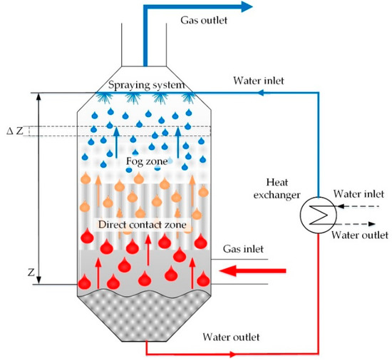
Figure 1.
Scheme of fog unit flows.
The mathematical model of the fog unit consists of equations describing flows and processes. In this study, the mathematical model is elaborated taking into account the following assumptions:
- Droplet distribution is monodispersed and has a defined starting diameter of droplets;
- Droplets are small, which leads to equal temperatures of droplets and their surface;
- Number of droplets in the unit is constant, convergence and disintegration of droplets due to their contact is not considered;
- Dry flue gas flow in the unit is constant;
- Droplets are spherical;
- Archimedes’ principle is not considered in droplet movement;
- Gas is ideal gas, to which the gas state equation applies [20].
In flue gas flow, temperature changes are determined by heat transfer between gas and water droplets in convection, vapor mass transfer from gas to droplets in the case of condensation, and from droplets to gas in evaporation. The driving force of convective heat transfer is the difference between gas temperature and water droplet temperature. Mass transfer is determined by the difference between the vapor partial pressure on droplets and in the gas flow. Mass transfer is related to latent heat release on droplets in condensation or latent heat transfer to gas. Gas temperature changes in the fog unit can be described using Equation (1).
Ranz and Marshall correlations are used for calculations of heat and mass transfer coefficients, which are offered in the paper [28]:
The following equations are used for calculations of similarity numbers:
Mass transfer coefficient’s βc, m/s recalculation to βp, and kmol/N·s
when droplets move through the unit, they come in contact and converge or disintegrate. It is assumed in the model that the number of droplets in the unit is constant. This means that the same number of droplets formed during collision and reduced when droplets converge is the same. The number of droplets is determined using Equation (6) as follows:
Water in the unit is in dispersed (droplets) form and the temperature of the water is equal to the droplet temperature, which increases starting from the spraying location to the outlet in the bottom part. Temperature changes occur due to heat transfer from gases to water droplets. They can be determined by Equation (7) as follows:
The Drodlet diameter changes in the unit are related to vapor transfer from gas to droplet surface in condensation or from droplet surface to gas, if evaporation occurs. The driving force of processes is the partial pressure difference between the partial pressure of vapor in gas flow and the partial pressure on the droplet surface. The partial pressure on the droplet surface corresponds to the vapor saturation pressure in droplet temperature. During condensation, the pressure difference is positive, water vapor moves from gases to droplets and condensates there, resulting in an increase of droplet diameter. During evaporation, the process occurs in the opposite direction. Droplet diameter changes can be described using Equation (8) as follows:
To determine saturated vapor partial pressure, Equation (9) improved by O. Toten is used [29] as follows:
Partial pressure of vapor in gas flow is determined by using the moisture content of gas as follows:
When looking at the vertical movement of a droplet in gas flow, several velocities are encountered. They are settling velocity of droplet in gas ur (terminal velocity), gas flow velocity ug, and droplet velocity in the unit ud. The real droplet velocity in flow determines the time during which the droplet is inside the unit. As velocity is a vectoral quantity, it is characterized by value and direction. In counter flow systems, where gas flow is the inverse to droplet movement, it is exposed to additional frontal resistance force created by flue gas. This force reduces droplet velocity ud and there can be cases where flow moves in an opposite direction. This should be considered in the case of small diameter droplets, because it is connected with droplets being carried away with gases. The normal operation of the fog unit is possible, if ud ug. In counter-flow unit droplet velocity changes are described by Equation (11) as follows:
For spherical drop, terminal velocity is determined by the balance of gravitational and resistance forces as follows:
Calculations are complicated by the fact that drag coefficient (CD) changes are determined using different laws and each law applies to a range of Reynolds number (Re) changes. Widening of the range of Re changes makes theoretical relationships become less precise, and therefore empirical or semi-empirical drag coefficient calculation equations are used in practice. Equations differ in terms of degrees of complexity and include constants [30]. Empirical relationships are based on one or another theoretical laws and, in most cases, it is Stokes law [31]. Establishing a uniform relationship for a wide range of Re is essential in the modeling process and attention is focused on determining the relationship [32].
Equation (13) for the Re range 0.1 ≤ Re ≤ 3·105 has been offered in the work of Shilyaev et al. [33]
Because drag coefficient depends on the droplet falling mode, then, it is necessary to know the Re number describing the movement regime for its determination as follows:
In calculations of the model, a step-by-step approximation (iteration) method is used. The Re value is assumed and drag coefficient is calculated using Equation (13). The relative velocity of droplets is calculated using Equations (12), and Equation (14) is used to calculate the Re value. If the value is different from that assumed, then, the calculation is repeated until the value obtained agrees with the assumed one in the chosen accuracy limits. Moisture content changes are caused by wet flue gas vapor condensation on the droplet surface. As a result, gas mass flow decreases, water mass flow increases, and changes in flow correspond to the amount of condensed vapor. The driving force of the condensation process is the difference between flow moisture partial pressure and saturation pressure.
The mathematical model consists of the main Equations (1), (7), (8), (11), (15), and related equations.
When starting modeling, the water temperature in the gas inlet, where current height (Z) Z = 0, is assumed because it is not known in the case of counter-flow. The calculated water temperature at the upper part of the unit, where Z = H (full height of the device), is compared with the sprayed water temperature. If values differ, then iteration is used, and water temperature is changed at the inlet of the unit.
2.2. Validation of Modeling Results
Validation was carried out by comparing experimental data and model results. Similar validation methods for comparing modeled and experimental data have been widely used regarding processes related to heat and mass transfer. For example, in the paper by Zheng et al. [34], a numerical algorithm was developed to describe droplet dynamics during dropwise condensation of moist air and applied to the entire condensation process. A single droplet growth model was made and applied to a limited surface. To validate results, dropwise condensation experiments were carried out at 94% and 80% relative humidities. Good agreements were obtained between the model and experiments, providing credibility to the model.
The capacity of the fog unit obtained with the model was, then, compared with the experimental results for the same operating regimes. The description of the experimental stand, setup, and full range of performed experiments are described in detail in the work of Priedniece V. et al. [14], as well as the effects of sprayed water flow rate, temperature, and drop size (based on nozzle type) on a fog unit’s performance were analyzed. The experimental stand consisted of a pellet boiler, a fog unit, pulp collection tank, flue gas pipes, and measurement equipment. The main parameters measured during experiments were flue gas temperature, water temperature, humidity of flue gas, pressure difference in flue gas pipe, and particulate matter concentration. All parameters were measured before and after the fog unit. The sprayed water flow rate, water temperature before and after scrubber, as well as the capacity of the fog unit were also measured. A total of 16 experimental regimes were compared with the model. They were performed at 20 kW pellet boiler capacity, which was the nominal capacity of the boiler used in the system, using varying ranges of main operating parameters of the fog unit. Regimes Nos. 1 to 6 were carried out using the largest nozzle MPL 1.51, regimes Nos. 7 to 13 were carried out using the medium nozzle MPL 1.12, and regimes Nos. 14 to 16 were carried out using the smallest nozzle MPL 0.77. Sprayed water temperature varied from 19.7 to 40.9 °C, at tests. The difference between results was calculated by having the experimental capacity of the fog unit as a reference value using Equation (16).
The set of main parameters used and compared is summarized in Table 1. The input parameters from the experimental dataset included the following: flue gas temperature before the fog unit (tg1), inlet water temperature (tw1), water flow rate (G), and water droplet diameter (dd0).

Table 1.
Main parameters of the study.
The flue gas temperature after the boiler was equal in 15 regimes with a value of 131 °C and one regime had a value of 135 °C, and therefore they are not included in the table. Three different nozzles were used during the experiments, providing similar water flows with different droplet diameters. The water flow rate ranged from ~50 to 249 l/h. The inlet water temperatures ranged from ~20 to ~40 °C. The experimental fog unit capacities ranged from 0.44 to 2.63 kW, while calculated fog unit capacities ranged from 0.44 to 2.41 kW. Water flow rate had a fluctuating effect on the fog unit capacity. Overall, increased water temperature led to a decrease in fog unit’s capacity, and therefore colder water is more suitable for spraying. On average, the water flow rate of ~150 l/h seemed to be quite optimal for heat recovery from flue gas.
To visualize the data and their differences, a graph which showed the differences in fog unit capacities due to water flows with changing inlet water temperatures in Figure 2 was made.
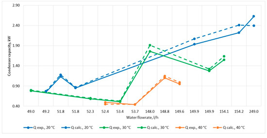
Figure 2.
Experimental and calculated fog unit capacities depending on water flows and inlet water temperatures.
As water flow rate and inlet temperature are two of the main parameters affecting the capacity of the fog unit, it is important to see their impact. As illustrated in Figure 2, the largest difference between calculated and experimental data is for capacities with water temperature 20 °C, with growing flow rate, and with an average difference of 8.16%. The most similar data are for the water temperature of 30 °C, at flow rates of ~50 l/h (2.70% on average). The difference between values is from 1.16% to 9.08%, the average difference between data is 4.88%. As the difference between values does not exceed 10%, it is concluded that the modeled data is in good agreement with the experimental data.
2.3. Condenser Optimization
Optimization is the process of determining the best design. Often optimization is performed using a combination of judgment, experience, modeling, opinions of others, and available theoretical materials. If parameters are affected by many variables, the determination of an optimum can be problematic based only on intuition.
Several empirical optimization methods exist nowadays. According to Taavitsainen V-M.T., the more widely used methods are the Nelder–Mead simplex strategy and the Box–Wilson strategy or the gradient method. The Box–Wilson method has several advantages and can be characterized as a flexible and understandable tool. The main principle of the strategy is to follow the path of the steepest ascent towards the optimal point. The method uses local polynomial modeling to find the direction of the steepest ascent. [35]
Frequently, a process in a small area of factor changes manages to describe a first order polynomial. If the equation found is adequate, then, the direction of the steepest ascent in this area is expressed by the polynomial coefficients found. The procedure is carried out by varying the factors in proportion to the numerical values of the respective coefficients and taking into account their signs. The advantageous point resulting from the course is assumed to be the center of the new design and the above procedure is repeated, obtaining a new polynomial and a new steep ascent. The process is continuous until the results of the experiment satisfy the experimenter. The regression equation coefficients can be found for the first order model as follows:
The obtained polynomial coefficients show the direction of the gradient relative to the encoded factors and one should always switch to natural factors after each series. Steps in the gradient attempts should not be changed in proportion to the coefficients bi but multiplied by the variation step δi. The base factor, xk, is used to determine the gradient step.
The new step in the gradient direction δ′k must be selected and the proportionality factor γ must be calculated for the base factor as follows:
The new steps for the other factors are calculated using the proportionality factor γ
The gradient step modes can be found by changing all the factors according to the new steps [35]
3. Results
Validation of the modeling results shows a good correlation with the experimental data. This confirms the hypothesis that the model can be used to determine operation data of the condenser using calculations. A numerical experiment was performed with the model for variable parameters in set boundaries. Calculation regimes were determined using a 2k experimental plan. The aim of the numerical experiment is to determine the relationships among fog unit capacity and five independent variables within their change limits:
- Flue gas flow Vg, Nm3/s;
- Flue gas temperature before the fog unit tg1, °C;
- Sprayed water flow rate G, l/h;
- Droplet diameter dd0, μm;
- Sprayed water temperature tw1, °C.
Each parameter was studied at two levels, i.e., at maximum and at minimum values. A total of 32 regimes were defined with an additional three regimes in the center of the plan. Regimes in the center of the plan include average values of all independent variables. The remaining regimes contain a mixture of minimal and maximal values of independent variables. The main values of variables are displayed in Table 2. The set values for each regime were chosen in random order. The regression equation describing data is obtained by processing numerical experiment matrix data in actual values in the program STATGRAPHICS Centurion 16.1.17, developed by Statgraphics Technologies Inc., located in The Plains, Virginia in the USA.
Qfu = 0.6458 + 165.8865·Vg + 0.0076·tg1 + 0.0067·G − 0.0014·dd0 − 0.0392·tw1
Table 2.
Factor change steps in optimization.
To develop the equation in coded values, the following recalculation equations are used:
In coded values Equation (12) is expressed as:
Y = 1.723 + 0.419·x1 + 0.189·x2 + 0.301·x3 −0.126·x4 − 0.196·x5
In the equation, x values are +1 for maximum values, −1 for minimum values, and 0 in the center of the plan.
The goal of optimization is to find a set of factors that provide the maximal value of Qfu. The steepest ascent or gradient (path) method is chosen for optimization. For this purpose, a model describing the effects of the main parameters is used excluding pairwise effects.
In the numerical experiment, the highest Qfu value is obtained when , , , and . It means that to find the optimal state, the values of Vg, tg1, and G must be increased but the dd0 and tw1 values must be reduced. It can be concluded from the regression equation in coded values, Equation (23), that gas flow impacts capacity the most, because it has the highest coefficient value.
The gas flow increase step is assumed and depending on it, change steps for other factors are determined. Optimization is started from the center point of the numerical experiment plan. The sequence of actions necessary is displayed in Table 2.
Coefficients bi values for parameter step calculations are obtained by determining partial differentials from Equation (18). A gradient direction step for the most significant factor Vg is assumed and steps for other factors are determined on that basis. Using factor change steps, the following regimes are defined and summarized in Table 3.
Table 3.
Regimes to determine optimum.
Condenser capacities in generated regimes are summarized in Table 3 and are linear in the center of the plan, which is confirmed by the difference in calculated condenser capacity. As evident in the results, the difference is practically constant. The obtained results can be used to define the starting direction of steepest ascent. They show the desirable value changes to reach the maximum possible capacity. The study shows that in order to provide a capacity increase, it is necessary to increase gas flow, water flow rate, flue gas temperature, as well as decrease droplet diameters and spray in water with lower temperature. The obtained results show the parameter change steps to achieve higher capacity of the condenser. In the studied unit, the maximum condenser capacity is limited by a flue gas flow value of 0.01 Nm3/s. This is determined by the capacity of the pellet boiler and combustion of quality fuel. Another essential condition limiting gas flow is the interaction between gas and droplets in the condenser. A higher water flow rate increases the removal of particulate matter.
The effects of certain parameters on the capacity of the fog unit can be displayed by response surface graphs. A response surface graph is a 3D representation of changes in the studied parameter (displayed on the Z axis) depending on two different parameters (displayed on the X and Y axes). In this case, there are two variable parameters and three constant parameters that affect the fog unit capacity. The response surface is calculated using the obtained regression Equation (21) using the program STATGRAPHICS Centurion 16.1.17. An example for Qfu changes due to varying G and Vg values is shown in Figure 3.
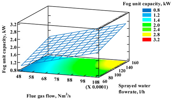
Figure 3.
Qfu response surface depending on varying Vg and G values.
The rest of the parameters in the equation are constant at values of the matrix center. The flue gas temperature is 115 °C, droplet diameter is 512.5 µm, and inlet water temperature is 25 °C. The obtained response surface shows a change in Qfu values from ~1.2 to ~2.8 kW. Vg and G values are in the range that was used in the matrix.
Similar graphs were made by changing the parameter displayed on the Y axis. When the flue gas temperature before the fog unit was displayed, the changes of Qfu ranged from ~1 to 2.6 kW. In the case of dd0, Qfu ranged from ~1.2 to ~2.4 kW. The remaining parameters were at center regime values, where G was 105 l/h.
When tw1 was displayed on the Y axis (Figure 4.), and the Qfu was in the range from ~1.2 to ~2.6 kW. The highest value of the fog unit capacity displayed in response surfaces is 2.8 kW and the lowest value is 1 kW. The range of changes differs for separate parameter pairs. Vg is kept on all response surfaces, because it directly characterizes the capacity of the boiler.
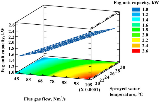
Figure 4.
Capacity of the fog unit (Qfu) response surface depending on varying gas volumetric flow rate (Vg) and water temperature (tw1) values.
4. Conclusions
A calculations model which describes the operation of a fog unit was developed and validated in this study. Validation was performed by comparing experimental and calculated fog unit capacities for the same regimes. Regimes were taken from an experimental dataset, for a boiler capacity of 20 kW. Good agreement was achieved among the data, with differences among results not exceeding 10%.
A numerical study was conducted to perform optimization. An experimental matrix for determination of the fog unit capacity including five main variables was made and analyzed. The variables were flue gas flow Vg, flue gas temperature before the fog unit tg1, sprayed water flow rate G, droplet diameter dd0, and sprayed water temperature tw1. The boundaries of the parameters were set considering the results of the experiments and they were applicable to boiler capacities from 10 to 20 kW.
The path of the steepest ascent was the optimization method used in the study, where the main parameter was Vg. The obtained results show the parameter change steps to achieve higher capacity of the condenser. In the studied unit, the maximum condenser capacity is limited by a flue gas flow value of 0.01 Nm3/s. This is determined by the capacity of the pellet boiler and combustion of quality fuel. Another essential condition limiting gas flow is the interaction between gas and droplets in the condenser. A higher water flow rate increases the removal of particulate matter.
The main results of the data analysis and optimization show that the fog unit capacity has a linear growing trend. However, it is not supported by experimental results, because the fog unit system has its limits regarding water flow rate, becoming less efficient when flow rate used in the experiments exceeds 200 l/h. The response surface graphs for the studied parameters’ range show that water flow rate is another main parameter that contributes to achieving the highest fog unit capacities, along with flue gas flow.
The performed condenser optimization study can be viewed as a basis for further studies which use more complex parameter models and repeated numerical experiments.
The mathematical model could be improved in the future. Currently, it has been validated for analyzing heat and mass transfer from boilers with capacity from 10 to 20 kW for a sprayed water flow rate from ~50 to 250 l/h and sprayed water temperature from 20 to 40 °C. The application range should be increased to make it more suitable for describing different heat and mass transfer situations that can occur in the scrubber. Additional improvement is related to particulate matter modeling. Although it was not studied in detail in this paper, it is included in the mathematical model. The results from the model that have been achieved so far using the experimental data as input for particulate matter modeling vary from the actual results. In order to achieve more accurate results, several equations could be included in the model describing the water spraying process, as well heat and mass transfer in the scrubber.
Author Contributions
Conceptualization, D.B., V.K. and I.V.; methodology, I.V., V.K., V.P.; software, R.R., A.Ņ., E.L.; validation, V.P., I.V.; formal analysis, V.P.; investigation, V.K., V.P.; resources, V.K.; data curation, I.V., V.P.; writing—original draft preparation, V.K., I.V., V.P.; writing—review and editing, D.B.; visualization, V.K.; supervision, D.B.; project administration, D.B.; funding acquisition, D.B. All authors have read and agreed to the published version of the manuscript.
Funding
This research was funded by the European Regional Development Fund project "Individual Heating with Integrated Fog Unit System (IFUS)" 1.1.1.1/16/A/015.
Conflicts of Interest
The authors declare no conflict of interest.
Nomenclature
| α | convective heat transfer coefficient, W/m2·K |
| βp | mass transfer coefficient, kmol/N·s |
| βc | mass transfer coefficient, m/s |
| λg | gas thermal conductivity, W/m·K |
| μg | gas dynamic viscosity, kg/m·s |
| ρw | water density, kg/m3 |
| νg | gas kinematic viscosity, m2/s |
| ω | absolute humidity, kg/kg d.g. |
| cpg | specific heat capacity of gas, J/kg·K |
| cpw | specific heat capacity of water, J/kg·K |
| cpv | specific heat capacity of vapor, J/kg·K |
| dd | diameter of droplet, m |
| ddo | initial diameter of droplet, μm |
| Dv | vapor diffusion coefficient, m2/s |
| mg | mass flow rate of gas, kg/s |
| Mv | molecular weight of vapor, kg/kmol |
| nd | number of drops, 1/s |
| pb | partial pressure of vapor in gas bulk, Pa |
| psat | partial pressure at the drop surface, Pa |
| Qfu | capacity of the fog unit, kW |
| ΔQ | difference between experimental and calculated capacity of the fog unit, % |
| Qfu exp. | experimental capacity of the fog unit, kW |
| r | heat of vaporization, J/kg |
| Ru | universal gas constant 8.314, J/mol·K |
| T | gas temperature, K |
| tg | gas temperature, °C |
| tw | water temperature, °C |
| ud | droplet velocity, m/s |
| ug | gas velocity, m/s |
| Vw | water volumetric flow rate, m3/s |
| Vg | gas volumetric flow rate, Nm3/s |
| CD | drag coefficient |
| H | height of device, m |
| Nu | Nusselt number |
| Pr | Prandtl number |
| Re | Reynolds number |
| Sh | Sherwood number |
| Sc | Schmidt number |
| Z | coordinate |
References
- Fernandes, U.; Costa, M. Particle emissions from a domestic pellets-fired boiler. Fuel Process. Technol. 2012, 103, 51–56. [Google Scholar] [CrossRef]
- Balmes, J.R. Household air pollution from domestic combustion of solid fuels and health. J. Allergy Clin. Immunol. 2019, 143, 1979–1987. [Google Scholar] [CrossRef] [PubMed]
- Villeneuve, J.; Palacios, J.; Savoie, P.; Godbout, S. A critical review of emission standards and regulations regarding biomass combustion in small scale units. Bioresour. Technol. 2012, 111, 1–11. [Google Scholar] [CrossRef] [PubMed]
- Directive 2009/125/EC of the European Parliament and of the Council of 21 October 2009 Establishing a Framework for the Setting of Ecodesign Requirements for Energy-Related Products. Available online: https://eur-lex.europa.eu/legal-content/EN/ALL/?uri=CELEX%3A32009L0125 (accessed on 15 March 2020).
- Bianchini, A.; Pellegrini, M.; Rossi, J.; Saccani, A.C. Theoretical model and preliminary design of an innovative wet scrubber for the separation of fine particulate matter produced by biomass combustion in small size boilers. Biomass Bioenergy 2018, 116, 60–71. [Google Scholar] [CrossRef]
- Blumberga, D.; Veidenbergs, I.; Romagnoli, F.; Rochas, C.; Zandeckis, A. Bioenergy Tehnologies; Institute of Energy Systems and Enviroment: Riga, Latvia, 2011; p. 272. [Google Scholar]
- Kirsanovs, V.; Zandeckis, A.; Veidenbergs, I.; Blumbergs, I.; Gedrovics, M.; Blumberga, D. Experimental Study on the Optimisation Burning Process in the Small Scale Pellet Boiler due Air Supply Improvement. Agron. Res. 2014, 12, 499–510. [Google Scholar]
- Chen, H.; Zhou, Y.; Cao, S.; Li, X.; Su, X.; An, L.; Gao, D. Heat exchange and water recovery experiments of flue gas with using nanoporous ceramic membranes. Appl. Therm. Eng. 2017, 110, 686–694. [Google Scholar] [CrossRef]
- Cao, E. Heat Transfer in Process Engineering; McGraw-Hill Education: New York, NY, USA, 2009. [Google Scholar]
- Zhao, S.; Yan, S.; Wang, D.K.; Wei, Y.; Qi, H.; Wu, T.; Feron, P. Simultaneous heat and water recovery from flue gas by membrane condensation: Experimental investigation. Appl. Therm. Eng. 2017, 113, 843–850. [Google Scholar] [CrossRef]
- Wei, M.; Fu, L.; Zhang, S.; Zhao, X. Experimental investigation on vapor-pump equipped gas boiler for flue gas heat recovery. Appl. Therm. Eng. 2019, 147, 371–379. [Google Scholar] [CrossRef]
- Ramanauskas, V.; Miliauskas, G. The water droplets dynamics and phase transformations in biofuel flue gases flow. Int. J. Heat Mass Transf. 2019, 131, 546–557. [Google Scholar] [CrossRef]
- Chien, L.-H.; Xu, J.-J.; Yang, T.-F.; Yan, W.-M. Experimental study on water spray uniformity in an evaporative condenser of a water chiller. Case Stud. Therm. Eng. 2019, 15, 100512. [Google Scholar] [CrossRef]
- Priedniece, V.; Kalnins, E.; Kirsanovs, V.; Dzikevics, M.; Blumberga, D.; Veidenbergs, I. Sprayed Water Flowrate, Temperature and Drop Size Effects on Small Capacity Flue Gas Condenser’s Performance. Environ. Clim. Technol. 2019, 23, 333–346. [Google Scholar] [CrossRef]
- Rahimi, A.; Niksiar, A.; Mobasheri, M. Considering roles of heat and mass transfer for increasing the ability of pressure drop models in venturi scrubbers. Chem. Eng. Process. Process. Intensif. 2011, 50, 104–112. [Google Scholar] [CrossRef]
- Saari, J.; Afanasyeva, S.; Vakkilainen, E.K.; Kaikko, J. Heat Transfer Model and Optimization of a Shell-And-Tube District Heat. In Proceedings of the 27th International Conference on Efficiency, Cost, Optimization, Simulation and Environmental Impact of Energy Systems (ECOS 2014), Turku, Finland, 15–19 June 2014; pp. 15–19. [Google Scholar]
- Wang, X.; Zhuo, J.; Liu, J.; Li, S. Synergetic process of condensing heat exchanger and absorption heat pump for waste heat and water recovery from flue gas. Appl. Energy 2020, 261, 114401. [Google Scholar] [CrossRef]
- Hossain, M. Heat and Mass Transfer. Modeling and Simulation; IntechOpen: London, UK, 2011. [Google Scholar]
- Rutgers, J. Dynamic Modeling of a Heat Exchanger, Internship at Powerspex; University of Twente: Hengelo, The Netherlands, 2016. [Google Scholar]
- Shilyaev, M.I.; Khromova, E.M. Modeling of Heat and Mass Transfer and Absorption-Condensation Dust and Gas Cleaning in Jet Scrubbers; IntechOpen: London, UK, 2013. [Google Scholar]
- Macháčková, A.; Kocich, R.; Bojko, M.; Kunčická, L.; Polko, K. Numerical and experimental investigation of flue gases heat recovery via condensing heat exchanger. Int. J. Heat Mass Transf. 2018, 124, 1321–1333. [Google Scholar] [CrossRef]
- Barati, S.B.; Pionnier, N.; Pinoli, J.-C.; Valette, S.; Gavet, Y. Investigation spatial distribution of droplets and the percentage of surface coverage during dropwise condensation. Int. J. Therm. Sci. 2018, 124, 356–365. [Google Scholar] [CrossRef]
- Lee, S.W.; No, H. Droplet size prediction model based on the upper limit log-normal distribution function in venturi scrubber. Nucl. Eng. Technol. 2019, 51, 1261–1271. [Google Scholar] [CrossRef]
- Ahmadvand, F.; Talaie, M.R. CFD modeling of droplet dispersion in a Venturi scrubber. Chem. Eng. J. 2010, 160, 423–431. [Google Scholar] [CrossRef]
- Miliauskas, G.; Adomavičius, A.; Maziukienė, M. Modelling of water droplets heat and mass transfer in the course of phase transitions. I: Phase transitions cycle peculiarities and iterative scheme of numerical research control and optimization. Nonlinear Anal. Model. Control. 2016, 21, 135–151. [Google Scholar] [CrossRef]
- Mirzabeygi, P.; Zhang, C. Three-dimensional numerical model for the two-phase flow and heat transfer in condensers. Int. J. Heat Mass Transf. 2015, 81, 618–637. [Google Scholar] [CrossRef]
- Lin, L.; Chen, Y.; Wu, J.; Guo, Y.; Dong, C. Performance of flow and heat transfer in vertical helical baffle condensers. Int. Commun. Heat Mass Transf. 2016, 72, 64–70. [Google Scholar] [CrossRef]
- Morsi, E.; Mohamed, S. Optimization of Direct Contact Spray Coolers. Ph.D. Thesis, University of Wisconsin Madison, Madison, WI, USA, 2002. [Google Scholar]
- Monteith, J.L.; Reifsnyder, W.E. Principles of Environmental Physics. Phys. Today 1974, 27, 51. [Google Scholar] [CrossRef]
- Cheng, N.S. Comparison of formulas for drag coefficient and settling velocity of spherical particles. Powder Technol. 2009, 189, 395–398. [Google Scholar] [CrossRef]
- Yang, H.; Fan, M.; Liu, A.; Dong, L. General formulas for drag coefficient and settling velocity of sphere based on theoretical law. Int. J. Min. Sci. Technol. 2015, 25, 219–223. [Google Scholar] [CrossRef]
- Morrison, F.A. Data Correlation for Drag Coefficient for Sphere; Department of Chemical Engineering Michigan Technological University: Houghton, MI, USA, 2016. [Google Scholar]
- Shilyaev, M.I.; Khromova, E.M. Modeling of Heat and Mass Transfer and Absorption-Condensation Dust and Gas Cleaning in Jets Scrubbers. In Mass Transfer–Advances in Sustainable Energy and Environment Oriented Numerical Modeling; IntechOpen: London, UK, 2013; pp. 163–194. [Google Scholar]
- Zheng, S.; Eimann, F.; Philipp, C.; Fieback, T.; Gross, U. Modeling of heat and mass transfer for dropwise condensation of moist air and the experimental validation. Int. J. Heat Mass Transf. 2018, 120, 879–894. [Google Scholar] [CrossRef]
- Taavitsainen, V.-M.T. Experimental Optimization and Response Surfaces; IntechOpen: London, UK, 2011. [Google Scholar]


© 2020 by the authors. Licensee MDPI, Basel, Switzerland. This article is an open access article distributed under the terms and conditions of the Creative Commons Attribution (CC BY) license (http://creativecommons.org/licenses/by/4.0/).